Nonlinear Autoregressive Model for Stability and Prediction
Abstract
A proposed nonlinear autoregressive model was employed to predict daily new COVID-19 infections in Iraq. This model was applied to actual COVID-19 data from 3 months in 2022 and met the stability criteria set by the proposed nonlinear regression model, based on a model developed by Japanese scientist Ozaki. The primary objective of the article was to examine the stability of this proposed nonlinear time series model, aimed at assessing the model’s stability and determining its stability conditions. To achieve this, the article applied Ozaki’s method to convert the nonlinear model, which depends on a singular point, into a linear model that fulfills the stability conditions required for the study. The approximation method helped identify the singular point, its stability conditions, and the limit cycle of the proposed model. The article also presented numerical case studies that satisfied the mathematical criteria for finding the singular point and its stability conditions. The findings indicated that such numerical case studies meeting stability conditions exist when the nonlinear function is decreasing, as illustrated in both Ozaki’s model and the proposed model. The proposed model was applied to COVID-19 data from Iraq over a 3-month period in 2022. This data was transformed into a stable form, and a Python program used the converted real data and proposed model to estimate the real parameters of the first-order model, fulfilling the established stability conditions and forecasting future new cases of the disease, which was the research’s main goal. The statistical criteria used in the fifth paragraph of the research are the Akaike information criterion (AIC), Bayesian information criterion (BIC), and normalized Bayesian information criterion (NBIC).
1. Introduction
The primary objective of studying various time series models is to enable the prediction of future observations of the studied phenomenon under investigation. It is essential for the time series used in predictions to be stable. The proposed study model is composed of two parts: a linear part and a nonlinear part, which is a decreasing rational function over time. This model is similar to and simulates the exponential autoregressive model. We applied the local linearization technique to get an approximate linear model nearly the singular point. The “singular point” was found first for the proposed model, followed by the stability criteria of the singular point, and third, the stability criteria of a limit cycle.
The theoretical aspect of the local linear approximation method is demonstrated using Example 1, which includes the orbits of the proposed first-order model and shows how it meets the stability condition. We utilized MATLAB programs to plot the paths of the proposed first-order model with various initial values. Example 1 satisfies the condition for the stability of the singular point, whereas Example 2 does not. For detailed MATLAB programs related to these examples (see Appendix A).
The model proposed in this research is a new nonlinear autoregressive model that simulates the exponential autoregressive model proposed by the Japanese scientist Ozaki, which was used to predict the number of new COVID-19 infections in Iraq by using real data of COVID-19 disease for three consecutive months of the year 2022 (the COVID-19 series real data between April 1, 2022, and June 30, 2022) obtained from the website of the World Health Organization (https://www.who.int/countries/irq/) (see Appendix B).
The study’s model was employed to analyze actual COVID-19 infection time series data in Iraq for a 3-month period in 2022. The data time series was transformed into a stable time series data by taking the natural logarithm and first difference; we used programs in Python to fit study data and estimate the parameters of the proposed first-order nonlinear model that satisfied stability conditions.
The MATLAB program was employed with various initial values to plot the paths of the proposed model, using real parameters obtained from the Python program that align with the data and ensure the model meets the stability condition (see Appendix C).
The Python program was used to estimate the true parameters of the studied model, which fulfills the condition of stability with the transformed data, and used to predict the values within the study period achieved (see Appendix D).
The Python program was utilized to estimate the real parameters of the suggested model using the original data and to predict future values of new COVID-19 infections in Iraq (see Appendix E).
1.1. Literature Review
The definition of time series can be found in References [1–3]. The definition of an autoregressive model for a p-order time series in discrete time is available in References [4–6]. The proposed Ozaki model, an exponential nonlinear model of p-order, is defined in References [7–9]. Additionally, the Ozaki model, an exponential nonlinear model with parameter γ of p-order, is defined in References [10–13]. Researcher Ozaki utilized the technique of local linearization for nonlinear time series models as described in References [8, 14]. Ozaki also studied “nonlinear threshold autoregressive models” for nonlinear random vibrations in Reference [15]. A connection was discovered between the autoregressive order of the threshold model and the order of its autoregressive moving average approximation in [16]. The use of fractional ordering in models examining the interactions between glioblastoma multiforme (GBM) and the immune system (IS) was investigated in Reference. A mathematical model of partial financial awareness is introduced using the Caputo–Fabrizio (CF) framework in Reference [17]. A recent study explores the literature concerning a prominent numerical model of global economic growth, specifically a nonlinear microeconomic model of consciousness in Reference [18]. The six-constant Jeffrey model is employed to demonstrate the key characteristic of viscoelastic material deformation, which exhibits both liquid and solid properties simultaneously in Reference [19]. The flow of second-order micronanofluid through an exponentially curved Riga layer, with the presence of double Cattaneo–Christoph diffusion, was examined in Reference [20]. The flow of a Satterby–Casson fluid over an exponentially curved sheet was studied in a two-dimensional framework in Reference [21]. The SD-AR model, which is grounded in deep belief networks, is investigated to assess the stability of nonlinear time series in [22]. A study was carried out on a prediction model for COVID-19 cases based on a nonlinear neural network in [23]. New multiregion machine learning approaches for predicting the COVID-19 pandemic in Africa are explored in [24].
The research includes the following paragraphs in addition to the abstract and introduction, it contains the following paragraphs: the study model, the local linear approximation method, study cases, application, conclusions, future work, and, in the last, references.
2. The Study Model
Our proposed study model simulates Ozaki’s self-exponential regression model, which we converted into a linear model using the local linearization approximation method. We identified the stability conditions for the model’s singular point, achieving them as demonstrated in Example 1 of the study cases. We then applied the model to real data on new daily COVID-19 infections in Iraq in 3 months in the year 2022, estimating real parameters for the first-order model using a spatial Python program that satisfies the identified stability conditions. Using the suggested model, we predicted the daily number of new infections for the next 10 days after the study period.
3. The Local Linearization Method
We used the local linearization method for determining the stability of the proposed model is an approximate one. This paragraph covers the theoretical aspects of the research related to the local linearization approximation method. It includes the identification of the singular point of the proposed model from the first order to the general order, as well as determining the stability conditions for the singular point of the proposed model for both the first and second orders. Additionally, it addresses the stability conditions for the limit cycle of the proposed model for both the first and second orders. These singular-point stability conditions for the first-order model will be applied in the case study section, Example 1, and in the practical application with real data on the daily new COVID-19 infections in Iraq. We used the proposed model for forecasting, as it meets the stability conditions.
3.1. Singular Point Z
Since εt = 0, Z = f(Z).
Therefore, Z = v1 + u1(1/Z + 1)]Z.
Also, (Z ≠ 0) and (u1 ≠ 0).
Since εt = 0, Z = f(Z).
Therefore, Z = [v1 + u1(1/Z + 1)]Z + [v2 + u2(1/Z + 1)]Z.
3.2. Singular Point Stability
The stability criteria of a singular point were constructed based on
ws = Z + Zs, for all s = t; t − 1
If the root of (8) lies in a unit circle, then (8) is a stable linear model of one order.
In symbols, |n1| = |m1| < 1.
The stability condition for singular point Z of (4) is as follows:
Therefore, v2 − m1v − m2 = (v − n1)(v − n2) = 0 of ((10)).
Then, m1 = (n1 + n2), m2 = −n1n2.
Since the roots are n1, n1, of the equation that v2 − m1v − m2 = 0
Therefore, ∀i = 1, 2, |ni| < 1, is a stability condition.
3.3. A Limit Cycle
The study proposed the model in Equation (4). The formula is wt = wt; ⋯; wt+q, εt = 0.
4. Case Studies
This part of the research includes two illustrations (referred to as Examples 1 and 2), that are used to identify the singular point of the proposed model, apply stability restrictions, and plot the orbits of the first-order models. Also, we can see Appendix A of the MATLAB programs, which shows the study model orbits plot for Examples 1 and 2. The criterion for the case studies is Equation (8), which is the condition for the stability of the singular point of the first order of the proposed model, which was derived. The programs used in the MATLAB language (Appendix A) assume optional real constants and do not determine whether or not the special criterion is met. By Equation (8), for example, the MATLAB program for Example 1 has real optional constants that satisfy the condition of Equation (8). It draws the orbits of the stable model for different initial values that settle at the singular nonzero point. The MATLAB program for Example 2 has real optional constants that do not meet the criterion of Equation (8). and draws the orbits of the unstable model for different initial values that move away from the singular nonzero point.
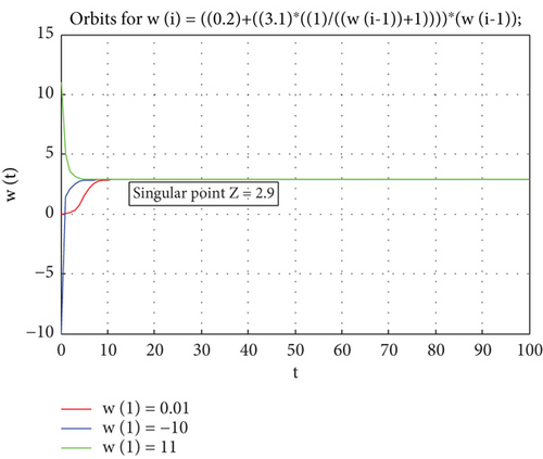
Example 1. Let us suppose that we have the given model.
While the real constants are v1 = 0.2, u1 = 3.1.
By using Equation (3), we derive that the singular point is
When Z = 2.9 and by using (8), Zt = 0.4Zt−1 ( ∗)
Therefore, Z = 2.9 is stable because the root n1 = 0.4 of equation ( ∗) is in a unit circle.
Therefore, Figure 1 displays the stability of the proposed model with different initial values w(1) = 0.01; w(1) = −10; w(1) = 11.
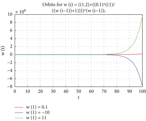
Example 2. If v1 = 1.2, u1 = 0.1, in Equation (2), then wt = [1.2 + 0.1(1/wt−1 + 1)]wt−1 + εt
By utilizing Equation (3), we determine that the singular point is
When Z = −1.5 and by using (8), we get that Zt = 1.6Zt−1
Therefore, Z = −1.5 is unstable (the root (n1 = 1.6) and is outside a unity circle.
Therefore, Figure 2) shows the model orbits that are unstable in different initial values.
5. Application
5.1. Description of the Data Utilized in the Study
The research made use of data obtained from the website of the World Health Organization (https://www.who.int/countries/irq/), which provides information on the daily count of new COVID-19 cases in Iraq between April 1, 2022, and June 30, 2022. The dataset comprises 91 observations, representing the number of new cases reported each day during this specific timeframe. The dataset’s lowest value occurred on May 4, 2022, with 40 new cases reported, whereas the highest value was recorded on June 30, 2022, with 2628 new cases reported, and to access the data used in the study, please refer to Appendix B.
Figure 3 displays the COVID = yt series data between April 1, 2022, and June 30, 2022.
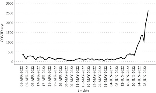
By utilizing the SPSS program to analyze the graph of the primary COVID-19 data series as shown in Figure 3, it becomes evident that the data is exhibiting growth, following an exponential pattern, and displaying instability.
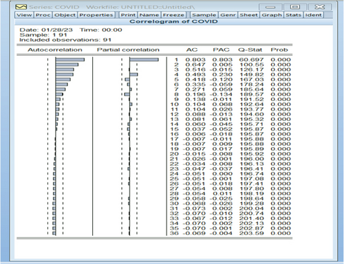
Through the utilization of the Eviews9 software, an analysis was conducted on the initial COVID-19 dataset (yt) using autocorrelation and partial autocorrelation functions, as depicted in Figure 4. The observation made from this analysis was that the COVID-19 variable lacks stability.
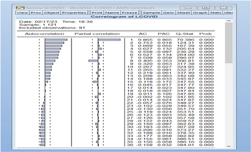
Due to the exponential nature of the original series, a fresh series named LCOVID was generated by logarithmically transforming the COVID-19 data. Subsequently, autocorrelation and partial autocorrelation functions were graphed for the LCOVID series. Nonetheless, upon observation, the newly derived LCOVID time series data was found to exhibit instability, as illustrated in Figure 5.
After applying the first difference to the original data by taking the natural logarithm, we obtained a new variable DLCOVID = log(yt) − log(yt−1) = Zt. The autocorrelation and partial autocorrelation functions were plotted for this new variable DLCOVID, as shown in Figure 6.
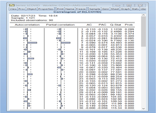
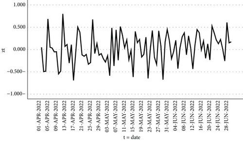
Figure 7 displays the resulting stable time series and can be used for predicting future observations. Figure 7 shows the series is stable of logarithms of the first difference of the original data that DLCOVID = Zt
5.2. Estimate the Parameters, Stability Condition, and Forcasted Prediction for the Study Model With Data
Programs in the Python language were used to estimate the values of the parameters suitable for the study data and the proposed nonlinear model and to achieve the stability conditions of the research model, which were found on the theoretical side in the third paragraph of the research, which is related to the results. We can see the Python program in the following link:https://colab.research.google.com/drive/1tQKVCqgIE1AzvAHQEdAO2fLNcEQD-khP.
5.2.1. Estimate the Parameters for Data and Model With Stability Condition
From the Python program, we estimate the parameters for the nonlinear proposed model that is suitable for the study data in our search.
The program starts by employing random initial values for the estimated real parameters.
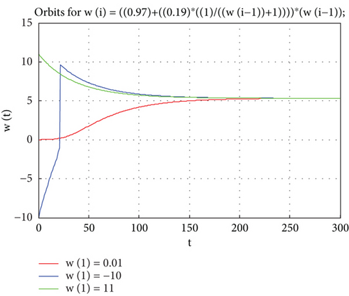
When Z = 5.3 and by using (8) to reach that, Zt = 0.97Zt−1 ( ∗).
Therefore, Z = 5.3 is stable because the root n1 = 0.97 of the equation ( ∗) is in a unit circle.
Also, we can see Appendix C for the MATLAB program which shows the study model orbits plot with estimated parameters for data that satisfied the stability condition, and Figure 8 explains the stability singular point Z = 5.3, with estimated real parameters c = v1 = 0.97, d = u1 = 0.19, that are suitable for the study data and study proposed model.
5.2.2. The Forecasting for the Study Model With Transformed Data
We were forecasting by using a proposed model with an estimate of the parameters that we found in the Python program in the following linkhttps://colab.research.google.com/drive/1tQKVCqgIE1AzvAHQEdAO2fLNcEQD-khP.
We can see Appendix D for transformed real data, forecasting data, and residuals of a nonlinear study model, and the statistical criteria are as follows:
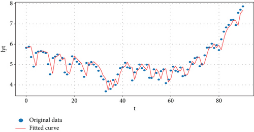
The mean squared error (MSE) = 0.11091933969757181; residual variance = 0.11341190912897792; Akaike information criterion (AIC) = 8.35345774885703; Bayesian information criterion (BIC) = −189.06060855996117, and normalized Bayesian information criterion (NBIC) = −2.077589105054518.
Figure 9 shows the transformed original data and forecasted data by using the study’s proposed model.
5.2.3. The Residual Test for the Study Model
The autocorrelation function and the partial autocorrelation function were found for the residuals of the model proposed in the first-order study for the transferred data, most of which fall within the limits of confidence, which indicates that the model agrees with the data used and the possibility of using it to predict future values. Figures 10 and 11 explain the autocorrelation and partial autocorrelation function graphs for the study model residuals.
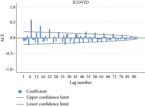
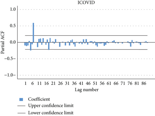
The residual is clearly white noise, indicating that the model is correct.
5.2.4. Forecasting COVID-19 Data for the Next Month That We Used by Using the Study Model
We can see the program in Python in the following link:https://colab.research.google.com/drive/1JnUQfIhl5ADcdZp_sBMSL0jORa6c6ONe.
The Python program found the forecasting of COVID-19 data by using the study model with the original data.
Figure 12 shows the forecasting of COVID-19 data by using the study model.

We can see Appendix E for the real data on COVID-19, forecasting data and residuals of anon linear study model.
5.2.5. The Predictions for the Study Model With Real Data
We can see the predictions for the study model with real data by using the Python program in the link (https://colab.research.google.com/drive/1JnUQfIhl5ADcdZp_sBMSL0jORa6c6ONe) for the next 10 days. Figure 13 explains the prediction of the real data on COVID-19 and the real data that we used in our search by using the study model for the next 10 days.
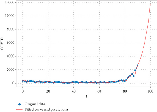
Table 1 shows the predictions for COVID-19 data by using the proposed study model for the next 10 days.
| t | 92 | 93 | 94 | 95 | 96 | 97 | 98 | 99 | 100 | 101 |
|---|---|---|---|---|---|---|---|---|---|---|
| Prediction of COVID | 3042 | 3524 | 4087 | 4742 | 5505 | 6394 | 7430 | 8636 | 10042 | 11680 |
6. Conclusions
- 1.
Our findings suggest that, according to the proposed Ozaki method for local linear approximation, the nonlinear component in the model should exhibit a decreasing trend to achieve numerical case studies that meet the stability conditions at a single point. Conversely, if the nonlinear function of the model is increasing, it is not possible to obtain numerical case studies that satisfy the stability conditions for a single point using this method.
- 2.
The model introduced in the study features a nonlinear component characterized by a decreasing function. This characteristic allowed us to find numerical examples that satisfied the stability conditions for the proposed model, as exemplified in Example 1 of the research.
- 3.
The first-order model suggested in the research, employing arbitrarily assigned real constants, can exhibit stability conditions, as illustrated in Example 1, or may fail to do so, as demonstrated in Example 2, with different initial values.
- 4.
The research demonstrates that the stability conditions theoretically established by the local linear approximation method are met by the proposed model.
- 5.
The proposed model was applied to actual data representing the time series of daily new COVID-19 infections in Iraq over a continuous span of 3 months in the year 2022. Employing a Python program, we estimated the values of the real parameter constants in the proposed model with the transformed data, satisfying the stability conditions, verifying the residuals, and subsequently enabling us to predict the forthcoming count of new COVID-19 infections for the subsequent 10 days.
- 6.
The findings from the analysis of real data using the proposed model for predicting new COVID-19 infections in Iraq indicated a rise in the predicted infection count, aligning with Figure 13 in the research, particularly at the onset of the sixth month of the year 2022. This alignment with the actual data suggests the suitability of the model for the study’s dataset.
7. The Future Recommendations
- 1.
The possibility of using the model proposed in the research for other real data in predicting future observations of the phenomenon studied by researchers in the future.
- 2.
Researchers can find stability conditions for the singular point, as well as conditions for the stability of the limit cycle for proposed models from the third order to the p order of the model proposed in our research.
- 3.
It is possible to propose and use models similar to our proposed model in this research, then find stability conditions, apply them to real data that fit the models, achieve stability conditions, and be used to predict future observations of the studied data for future researchers.
Conflicts of Interest
The authors declare no conflicts of interest.
Funding
There is no funding for this research.
Appendix A
MATLAB programs for case studies:
Example A1. clear
clc
close all;
sValus=[0.01-10 11];
colors=[′r′ ′b′ ′g′];
sh=[′-o-′ ′-.-′ ′-′]
figure(1);
hold
for j=1:3
w(1)=sValus(j);
t=0:100;
for i=2:length(t)
w(i)=((0.2)+((3.1) ∗((1)/((w(i-1))+1)))) ∗(w(i-1));
end
disp(′ t w[t]′)
disp([′t w′])
plot(t,w,′LineWidth′,2,′Color′,colors(j))
legend(′w(1)=0.01′,′w(1)=-10′,′w(1)=11′);
title(′Orbits for w(i)=((0.2)+((3.1) ∗((1)/((w(i-1))+1)))) ∗(w(i-1));′)
xlabel(′t′)
ylabel(′w[t]′)
grid on
end
hold
Example A2. clear
clc
close all;
sValus=[0.1-10 11];
colors=[′r′ ′b′ ′g′];
sh=[′-o-′ ′-.-′ ′-′]
figure(1);
hold
for j=1:3
w(1)=sValus(j);
t=0:100;
for i=2:length(t)
w(i)=((1.2)+((0.1) ∗((1)/((w(i-1))+1)))) ∗(w(i-1));
end
disp(′ t w[t]′)
disp([′t w′])
plot(t,w,′LineWidth′,2,′Color′,colors(j))
legend(′w(1)=0.1′,′w(1)=-10′,′w(1)=11′);
title(′Orbits for w(i)=((1.2)+((0.1) ∗((1)/((w(i-1))+1)))) ∗(w(i-1));′)
xlabel(′t′)
ylabel(′w[t]′)
grid on
end
hold
Appendix B
| t | COVID-19 |
|---|---|
| April 1, 2022 | 341 |
| April 2, 2022 | 358 |
| April 3, 2022 | 218 |
| April 4, 2022 | 134 |
| April 5, 2022 | 266 |
| April 6, 2022 | 280 |
| April 7, 2022 | 289 |
| April 8, 2022 | 274 |
| April 9, 2022 | 261 |
| April 10, 2022 | 151 |
| April 11, 2022 | 93 |
| April 12, 2022 | 207 |
| April 13, 2022 | 222 |
| April 14, 2022 | 248 |
| April 15, 2022 | 183 |
| April 16, 2022 | 204 |
| April 17, 2022 | 102 |
| April 18, 2022 | 92 |
| April 19, 2022 | 152 |
| April 20, 2022 | 224 |
| April 21, 2022 | 199 |
| April 22, 2022 | 171 |
| April 23, 2022 | 153 |
| April 24, 2022 | 110 |
| April 25, 2022 | 82 |
| April 26, 2022 | 161 |
| April 27, 2022 | 147 |
| April 28, 2022 | 168 |
| April 29, 2022 | 148 |
| April 30, 2022 | 135 |
| May 1, 2022 | 110 |
| May 2, 2022 | 83 |
| May 3, 2022 | 72 |
| May 4, 2022 | 40 |
| May 5, 2022 | 65 |
| May 6, 2022 | 45 |
| May 7, 2022 | 70 |
| May 8, 2022 | 55 |
| May 9, 2022 | 92 |
| May 10, 2022 | 126 |
| May 11, 2022 | 131 |
| May 12, 2022 | 162 |
| May 13, 2022 | 129 |
| May 14, 2022 | 126 |
| May 15, 2022 | 68 |
| May 16, 2022 | 102 |
| May 17, 2022 | 119 |
| May 18, 2022 | 149 |
| May 19, 2022 | 126 |
| May 20, 2022 | 113 |
| May 21, 2022 | 149 |
| May 22, 2022 | 78 |
| May 23, 2022 | 77 |
| May 24, 2022 | 118 |
| May 25, 2022 | 99 |
| May 26, 2022 | 71 |
| May 27, 2022 | 108 |
| May 28, 2022 | 118 |
| May 29, 2022 | 60 |
| May 30, 2022 | 71 |
| May 31, 2022 | 111 |
| June 1, 2022 | 135 |
| June 2, 2022 | 110 |
| June 3, 2022 | 105 |
| June 4, 2022 | 129 |
| June 5, 2022 | 84 |
| June 6, 2022 | 88 |
| June 7, 2022 | 117 |
| June 8, 2022 | 170 |
| June 9, 2022 | 151 |
| June 10, 2022 | 205 |
| June 11, 2022 | 212 |
| June 12, 2022 | 137 |
| June 13, 2022 | 151 |
| June 14, 2022 | 236 |
| June 15, 2022 | 344 |
| June 16, 2022 | 342 |
| June 17, 2022 | 413 |
| June 18, 2022 | 339 |
| June 19, 2022 | 385 |
| June 20, 2022 | 305 |
| June 21, 2022 | 515 |
| June 22, 2022 | 751 |
| June 23, 2022 | 932 |
| June 24, 2022 | 1061 |
| June 25, 2022 | 1328 |
| June 26, 2022 | 1345 |
| June 27, 2022 | 1039 |
| June 28, 2022 | 1905 |
| June 29, 2022 | 2212 |
| June 30, 2022 | 2628 |
Appendix C
Example A3. MATLAB program with estimate parameters for data and proposed model.
clear
clc
close all;
sValus=[0.01-10 11];
colors=[′r′ ′b′ ′g′];
sh=[′-o-′ ′-.-′ ′-′]
figure(1);
hold
for j=1:3
w(1)=sValus(j);
t=0:300;
for i=2:length(t)
w(i)=((0.97)+((0.19) ∗((1)/((w(i-1))+1)))) ∗(w(i-1));
end
disp(′ t w[t]′)
disp([′t w′])
plot(t,w,′LineWidth′,2,′Color′,colors(j))
legend(′w(1)=0.01′,′w(1)=-10′,′w(1)=11′);
title(′Orbits for w(i)=((0.97)+((0.19) ∗((1)/((w(i-1))+1)))) ∗(w(i-1));′)
xlabel(′t′)
ylabel(′w[t]′)
grid on
end
hold
Appendix D
| t | Log(yt) | Forecasting (log(yt)) | Residuals |
|---|---|---|---|
| 1 | 5.831882477 | 5.838648388 | −0.00676591 |
| 2 | 5.880532986 | 5.838648388 | 0.041884599 |
| 3 | 5.384495063 | 5.886145596 | −0.501650534 |
| 4 | 4.8978398 | 5.401719679 | −0.503879879 |
| 5 | 5.583496309 | 4.926089877 | 0.657406432 |
| 6 | 5.634789603 | 5.596103029 | 0.038686574 |
| 7 | 5.666426688 | 5.646196894 | 0.020229794 |
| 8 | 5.613128106 | 5.677092394 | −0.063964287 |
| 9 | 5.564520407 | 5.625042366 | −0.060521958 |
| 10 | 5.017279837 | 5.577569931 | −0.560290095 |
| 11 | 4.532599493 | 5.042862407 | −0.510262914 |
| 12 | 5.332718793 | 4.568827433 | 0.76389136 |
| 13 | 5.402677382 | 5.3511352 | 0.051542182 |
| 14 | 5.513428746 | 5.419482499 | 0.093946247 |
| 15 | 5.209486153 | 5.527667969 | −0.318181816 |
| 16 | 5.318119994 | 5.230722064 | 0.087397929 |
| 17 | 4.624972813 | 5.336871683 | −0.71189887 |
| 18 | 4.521788577 | 4.65921036 | −0.137421783 |
| 19 | 5.023880521 | 4.558248173 | 0.465632348 |
| 20 | 5.411646052 | 5.049314901 | 0.362331151 |
| 21 | 5.293304825 | 5.428244061 | −0.134939236 |
| 22 | 5.141663557 | 5.312625658 | −0.170962102 |
| 23 | 5.030437921 | 5.164440552 | −0.134002631 |
| 24 | 4.700480366 | 5.055725006 | −0.35524464 |
| 25 | 4.406719247 | 4.733076727 | −0.32635748 |
| 26 | 5.081404365 | 4.445627109 | 0.635777256 |
| 27 | 4.990432587 | 5.105543973 | −0.115111386 |
| 28 | 5.123963979 | 5.016617072 | 0.107346907 |
| 29 | 4.997212274 | 5.147141862 | −0.149929588 |
| 30 | 4.905274778 | 5.023244884 | −0.117970105 |
| 31 | 4.700480366 | 4.933359597 | −0.232879231 |
| 32 | 4.418840608 | 4.733076727 | −0.31423612 |
| 33 | 4.276666119 | 4.457492103 | −0.180825984 |
| 34 | 3.688879454 | 4.318300824 | −0.62942137 |
| 35 | 4.17438727 | 3.742211417 | 0.432175853 |
| 36 | 3.80666249 | 4.218134475 | −0.411471986 |
| 37 | 4.248495242 | 3.857743036 | 0.390752206 |
| 38 | 4.007333185 | 4.290714693 | −0.283381508 |
| 39 | 4.521788577 | 4.054465365 | 0.467323212 |
| 40 | 4.836281907 | 4.558248173 | 0.278033734 |
| 41 | 4.875197323 | 4.865896091 | 0.009301232 |
| 42 | 5.087596335 | 4.903950018 | 0.183646317 |
| 43 | 4.859812404 | 5.111596219 | −0.251783815 |
| 44 | 4.836281907 | 4.888906041 | −0.052624134 |
| 45 | 4.219507705 | 4.865896091 | −0.646388386 |
| 46 | 4.624972813 | 4.262326576 | 0.362646238 |
| 47 | 4.779123493 | 4.65921036 | 0.119913133 |
| 48 | 5.003946306 | 4.809997513 | 0.193948793 |
| 49 | 4.836281907 | 5.029827979 | −0.193546072 |
| 50 | 4.727387819 | 4.865896091 | −0.138508273 |
| 51 | 5.003946306 | 4.759396354 | 0.244549952 |
| 52 | 4.356708827 | 5.029827979 | −0.673119153 |
| 53 | 4.343805422 | 4.396670471 | −0.052865049 |
| 54 | 4.770684624 | 4.384037914 | 0.38664671 |
| 55 | 4.59511985 | 4.801744081 | −0.206624231 |
| 56 | 4.262679877 | 4.630002777 | −0.3673229 |
| 57 | 4.682131227 | 4.304605167 | 0.37752606 |
| 58 | 4.770684624 | 4.715127558 | 0.055557066 |
| 59 | 4.094344562 | 4.801744081 | −0.707399519 |
| 60 | 4.262679877 | 4.139724141 | 0.122955736 |
| 61 | 4.709530201 | 4.304605167 | 0.404925035 |
| 62 | 4.905274778 | 4.74192903 | 0.163345748 |
| 63 | 4.700480366 | 4.933359597 | −0.232879231 |
| 64 | 4.65396035 | 4.733076727 | −0.079116377 |
| 65 | 4.859812404 | 4.68756932 | 0.172243084 |
| 66 | 4.430816799 | 4.888906041 | −0.458089242 |
| 67 | 4.477336814 | 4.469214638 | 0.008122177 |
| 68 | 4.762173935 | 4.514746001 | 0.247427934 |
| 69 | 5.135798437 | 4.793420257 | 0.34237818 |
| 70 | 5.017279837 | 5.158708335 | −0.141428498 |
| 71 | 5.323009979 | 5.042862407 | 0.280147572 |
| 72 | 5.356586275 | 5.3416494 | 0.014936875 |
| 73 | 4.919980926 | 5.374453813 | −0.454472887 |
| 74 | 5.017279837 | 4.947738554 | 0.069541283 |
| 75 | 5.463831805 | 5.042862407 | 0.420969398 |
| 76 | 5.840641657 | 5.479222329 | 0.361419328 |
| 77 | 5.834810737 | 5.84720014 | −0.012389403 |
| 78 | 6.023447593 | 5.841507313 | 0.18194028 |
| 79 | 5.826000107 | 6.025655812 | −0.199655704 |
| 80 | 5.953243334 | 5.832905265 | 0.120338069 |
| 81 | 5.720311777 | 5.957126919 | −0.236815143 |
| 82 | 6.244166901 | 5.729711314 | 0.514455586 |
| 83 | 6.621405652 | 6.241071759 | 0.380333893 |
| 84 | 6.837332815 | 6.60913073 | 0.228202084 |
| 85 | 6.966967139 | 6.819744656 | 0.147222482 |
| 86 | 7.19142933 | 6.946170407 | 0.245258923 |
| 87 | 7.204149292 | 7.165046056 | 0.039103236 |
| 88 | 6.946013991 | 7.177448316 | −0.231434325 |
| 89 | 7.552237288 | 6.925736782 | 0.626500506 |
| 90 | 7.701652363 | 7.516798815 | 0.184853548 |
| 91 | 7.87397838 | 7.662439161 | 0.211539218 |
Appendix E
| t | COVID-19 | Forecasting COVID-19 | Residual |
|---|---|---|---|
| 1 | 341 | 378 | −37 |
| 2 | 358 | 378 | −20 |
| 3 | 218 | 398 | −180 |
| 4 | 134 | 235 | −101 |
| 5 | 266 | 137 | 129 |
| 6 | 280 | 291 | −11 |
| 7 | 289 | 307 | −18 |
| 8 | 274 | 317 | −43 |
| 9 | 261 | 300 | −39 |
| 10 | 151 | 285 | −134 |
| 11 | 93 | 157 | −64 |
| 12 | 207 | 89 | 118 |
| 13 | 222 | 222 | 0 |
| 14 | 248 | 239 | 9 |
| 15 | 183 | 270 | −87 |
| 16 | 204 | 194 | 10 |
| 17 | 102 | 218 | −116 |
| 18 | 92 | 100 | −8 |
| 19 | 152 | 88 | 64 |
| 20 | 224 | 158 | 66 |
| 21 | 199 | 242 | −43 |
| 22 | 171 | 213 | −42 |
| 23 | 153 | 180 | −27 |
| 24 | 110 | 159 | −49 |
| 25 | 82 | 109 | −27 |
| 26 | 161 | 76 | 85 |
| 27 | 147 | 168 | −21 |
| 28 | 168 | 152 | 16 |
| 29 | 148 | 177 | −29 |
| 30 | 135 | 153 | −18 |
| 31 | 110 | 138 | −28 |
| 32 | 83 | 109 | −26 |
| 33 | 72 | 78 | −6 |
| 34 | 40 | 65 | −25 |
| 35 | 65 | 28 | 37 |
| 36 | 45 | 57 | −12 |
| 37 | 70 | 34 | 36 |
| 38 | 55 | 63 | −8 |
| 39 | 92 | 45 | 47 |
| 40 | 126 | 88 | 38 |
| 41 | 131 | 128 | 3 |
| 42 | 162 | 133 | 29 |
| 43 | 129 | 170 | −41 |
| 44 | 126 | 131 | −5 |
| 45 | 68 | 128 | −60 |
| 46 | 102 | 60 | 42 |
| 47 | 119 | 100 | 19 |
| 48 | 149 | 119 | 30 |
| 49 | 126 | 154 | −28 |
| 50 | 113 | 128 | −15 |
| 51 | 149 | 113 | 36 |
| 52 | 78 | 154 | −76 |
| 53 | 77 | 72 | 5 |
| 54 | 118 | 71 | 47 |
| 55 | 99 | 118 | −19 |
| 56 | 71 | 96 | −25 |
| 57 | 108 | 64 | 44 |
| 58 | 118 | 107 | 11 |
| 59 | 60 | 118 | −58 |
| 60 | 71 | 51 | 20 |
| 61 | 111 | 64 | 47 |
| 62 | 135 | 110 | 25 |
| 63 | 110 | 138 | −28 |
| 64 | 105 | 109 | −4 |
| 65 | 129 | 103 | 26 |
| 66 | 84 | 131 | −47 |
| 67 | 88 | 79 | 9 |
| 68 | 117 | 83 | 34 |
| 69 | 170 | 117 | 53 |
| 70 | 151 | 179 | −28 |
| 71 | 205 | 157 | 48 |
| 72 | 212 | 220 | −8 |
| 73 | 137 | 228 | −91 |
| 74 | 151 | 140 | 11 |
| 75 | 236 | 157 | 79 |
| 76 | 344 | 256 | 88 |
| 77 | 342 | 382 | −40 |
| 78 | 413 | 379 | 34 |
| 79 | 339 | 462 | −123 |
| 80 | 385 | 376 | 9 |
| 81 | 305 | 429 | −124 |
| 82 | 515 | 336 | 179 |
| 83 | 751 | 581 | 170 |
| 84 | 932 | 856 | 76 |
| 85 | 1061 | 1066 | −5 |
| 86 | 1328 | 1217 | 111 |
| 87 | 1345 | 1528 | −183 |
| 88 | 1039 | 1548 | −509 |
| 89 | 1905 | 1191 | 714 |
| 90 | 2212 | 2200 | 12 |
| 91 | 2628 | 2558 | 70 |
Open Research
Data Availability Statement
The COVID-19 series real data in Iraq between April 1, 2022, and June 30, 2022, were obtained from the website of the World Health Organization (https://www.who.int/countries/irq/).


