In an ecological point of view, fears from predator cause physiological changes of prey population and these physiological changes may reduce the reproduction of prey. This paper deals with studying the effect of fear that is incorporated in the growth rate of prey on the dynamics of a delay ecological model consisting of two logistically growing prey species, namely, preyXand preyY, and a predator species. The predators take energy and biomass on predating on prey X as well as prey Y with extended Holling Type II functional response. We conduct a thorough analytical examination of the system, demonstrating the positivity and boundedness of the solutions. Criteria for the persistence of the model are founded. Seven biologically possible steady states are determined, and the local dynamics around the steady states based on the parameters are also investigated. Next, we investigated the occurrence of Hopf bifurcation around the prey X– and Y–free steady state, by taking the value of the time delay as a bifurcation parameter. Finally, we perform extensive numerical simulations to support the evidence of our analytical results and reveal the occurrence of Hopf bifurcation within the proposed model.

1. Introduction

In the recent years, the dynamic interaction between predators and their prey has been modeled by both a mathematician and biologist author [1–5]. In ecology, average number of eaten preys by one predator in a unit time is called functional response. Therefore, functional response is the important element to represent the dynamic relationship between predator population and prey population [6]. There are many types of functional response; among them is Holling Type II functional response which is characterized by decelerating intake rate [7, 8]. In nature, many predator species predate multiple species of prey. For example, lions usually predate many species of prey such as antelopes, buffaloes, crocodiles, giraffes, pigs, zebra, wild dogs, and wildebeest. Therefore, some mathematician authors investigate mathematical modeling for the dynamic interaction between one predator and multiple preys [3, 6]. Elettreby in [3] discussed the global stability and persistence of a one-predator and two-prey model. Fatah, Mustafa, and Shilan in [6] extended the Holling Type II functional response for n-preys. Population dynamics may be affected by many factors of natural environment like fear, harvesting, toxicity, stage structure, delay, cannibalism, antipredator skills, refuge, infectious illness, and other population-affecting elements [9–12].

Predation fears from predator causes physiological changes of prey population, and these physiological changes may reduce the reproduction of prey population [13]. Wang, Zanette, and Zou [14] considered a predator–prey model incorporating fear effect on reproduction of prey individuals; in their study, they noticed that the fear has no impact on the stability of the model when the system incorporates bilinear functional response, but the system becomes stable under fear effect, if it incorporates the Holling Type II functional response; based on their system, Pal et al. [15] considered a prey predator with fear effect and harvesting cooperation; they discussed the stability, Hopf bifurcation and Bogdanov–Takens bifurcation the system. Zhang et al. [16] considered an ecological model with fear effect and prey refuge; they showed that the effect of both factors can stabilize the system. For more results about fear effect, see [9, 17–20].

In predator–prey models, time delay on prey is the period of time between the prey predation and predator response to the predation. Haque et al. [21] investigated the effect of delay in a Lotka–Volterra-type predator–prey model with a transmissible disease in the predator species. Liu et al. [20] studied the dynamics of a predator–prey model with the effect of both fear and time delay. Abbas and Naji [22] considered and studied a food web model including two competing predator species and one prey species with Monod–Haldane functional response. For more results about time delay, see [23–26].

Based on the Lotka–Volterra-type predator–prey model, in the current work, we consider a two-prey–one-predator model incorporating the effect of fear in the growth rate of prey species and time delay between the prey predation and predator response to the predation. In Section 2, the details of the model formulation are given and some properties of the model’s solution are derived. In Section 3, the existence conditions of all feasible steady states are found. In Section 4, local stability analysis of the model and Hopf bifurcation near steady states are studied. In Section 5, discovering the impact of fear and time delay and illustrating the analytical finding that observed in this work are done through preforming some numerical simulations. Finally, in Section 6, a brief conclusion on the total work is given.

The novelty of this paper is discovering the effect of fear in prey and time delay between the prey predation and predator response to the predation on the dynamics of an ecological model including two different prey species and one predator species and the model incorporating the Holling Type II functional response which is modified by authors in [6].

2. The Mathematical Model and Its Solution Properties

Suppose a predator consumes two species of prey, namely, prey X and prey Y. To represent the dynamic interaction between the species, we derive a mathematical model based on the following assumptions:

i.
The number of prey X and prey Y and predator at instant time t is denoted by X(t), Y(t) and P(t), respectively.
ii.
Both species of prey X and prey Y grow logistically with intrinsic growth rate r₁ and carrying capacity K₁ for prey X and intrinsic growth rate r₂ and carrying capacity K₂ for prey Y.
iii.
The effect of fear is incorporated in the intrinsic growth rate of prey population due to the predator [27]. The intrinsic growth rates of prey X and prey Y are decreased, and they multiplied by 1/(1 + f₁P) and 1/(1 + f₂P), respectively, where f₁ and f₂ are levels of fear due to prey X and prey Y response to antipredators, respectively.
iv.
Prey X and prey Y are killed directly by predator species according to extended Holling Type II functional response α₁P/(1 + α₁T₁X + α₂T₂Y) and α₂P/(1 + α₁T₁X + α₂T₂Y), respectively, where α₁ and α₂ are the predator’s search efficiency for prey X and prey Y, respectively, and T₁ and T₂ are the predator’s average handling times of prey X and prey Y, respectively.
v.
The period between the prey predation and predator response to the predation is denoted by τ.
vi.
The predator number decreased by natural death with rate d and intraspecific competition between individuals of predators with rate c.
vii.
The biomass of prey X and prey Y is converted to the biomass of predator with rates e₁ and e₁, respectively.

Then, such interaction dynamics can be modeled mathematically through the following system of differential equations:

(1)

where X(0) > 0, Y(0) > 0, and P(0) > 0.

Functions F, G, and H in System (1) are continuous and has partial derivatives on the space R³, and hence, System (1) satisfies the Lipschitzian condition. Therefore, by uniqueness theorem, it has unique solution. Further, the time derivative of X, Y, and Z are zero in YZ‑plane, XZ‑plane, and XY‑plane, respectively. Therefore, if the solution initiates at a nonnegative point, then the components X, Y, and Z of the solution points of System (1) cannot cross any coordinates of the solution points. Hence, components X, Y, and Z of solution points are always nonnegative. Further, some properties of solutions of System (1) are proved in the following lemma and theorems.

Lemma 1. In System (1), the following inequalities are satisfied:

a.
, , and .
b.
If R_e < 1, then , , and .
c.
If X_Min > 0, then .
d.
If Y_min > 0, then .
e.
If P_Min1 > 0, then .
f.
If P_Min2 > 0, then .
g.
If X_Min > 0, Y_Min > 0, and P_Min1 > 0, then .

where

Proof 1 (a). From the first and second equations in System (1), it gets

So, and , and then

Thus, .

Proof 2 (b). By applying Part (a) in the third equation of System (1), it also gets

If R_e < 1, then , and hence, System (1) can be reduced to the following equations:

Solving above equations it gets and .

Proof 3 (c). Applying Part (b) in the first equation of System (1), it gets

So, if X_Min > 0, then

Proof 4 (d). Applying Part (b) in the second equation of System (1), it gets

Therefore, if Y_min > 0, then .

Proof 5 (e, f, and g). Applying Part (c) and Part (d) in the third equation of System (1), the following inequalities are obtained:

So,

The proof is completed.

From Lemma 1 (a), the following theorem can be derived.

Theorem 1. All solutions of System (1) are bounded.

Also, from Lemma 1 (c–g), the following theorem can be derived.

Theorem 2. If P_Min1 > 0 and P_Min2 > 0, then System (1) persists.

3. Existence of Steady States

System (1) has at most the following steady states:

1.
Extinct steady state S₁(0, 0, 0)
2.
The axial steady state S₂(K₁, 0, 0)
3.
The axial steady state S₃(0, K₂, 0)
4.
Predator-free steady state S₄(K₁, K₂, 0)

Prey Y–free steady state S₅(X₅, 0, P₅), where

and X₅ is root for the function

with

Suppose the following inequalities hold:

(2)

Clearly, H₁(K₁) < 0, so there is a root of H₁(X) in ]X_Min, K₁[.

Consequently, S₅(X₅, 0, P₅) exists if Condition (2) holds.

5.
Prey X–free steady state S₆(0, Y₆, P₆), where

is root for the function

with

Suppose the following inequalities hold:

(3)

Clearly, H₂(K₂) < 0, so there is a root of H₁(X) in ]Y_Min, K₂[.

Consequently, S₆(0, Y₆, P₆) exists if Condition (3) holds.

6.
Coexistence steady state S₇(X₇, Y₇, P₇)

where X₇, Y₇, and P₇ are positive solutions of the following equations:

(4)

Therefore, S₇(X₇, Y₇, P₇) exists if System (4) has positives solution.

4. Local Stability and Hopf Bifurcation

To investigate the locally asymptotically stable (LAS) for each steady state, we Linearize system (1) near a point(X, Y, P). Using the perturbed variables U(t) = X(t) − X and V(t) = Y(t) − YW(t) = P(t) − P, System (1) can be linearized as follows:

where

and

with

The eigenvalues of variational matrix at S₂(K₁, 0, 0) are r₁ > 0, r₂ > 0, and −d.

The eigenvalues of variational matrix at S₂(K₁, 0, 0) are −r₁ < 0, r₂ > 0, and (e₁α₁K₁/(1 + α₁T₁K₁)1 + α₁T₁K₁) − d.

The eigenvalues of variational matrix at S₃(0, K₂, 0) are r₁ > 0, −r₂ < 0, and (e₂α₂K₂/(1 + α₂T₂K₂)1 + α₂T₂K₂) − d.

Therefore, S₁(0, 0, 0), S₂(K₁, 0, 0), and S₃(0, K₂, 0) are saddle points.

The eigenvalues of variational matrix at S₄(K₁, K₂, 0) are −r₁ < 0, −r₂ < 0, and (1/d)(R_e − 1).

Thus, S₄(K₁, K₂, 0) is LAS, if and only if R_e < 1.

Theorem 3. For 0≤τ < (1/y₀)sin⁻¹(A₁y₀/C₁), S₅(X₅, 0, P₅) is LAS, if the following conditions hold:

(5)

(6)

Further, in addition to Conditions (5) and (6), if the following conditions hold

(7)

(8)

then at τ = (1/y₀)sin⁻¹(A₁y₀/C₁), System (1) undergoes a Hopf bifurcation near S₅(X₅, 0, P₅), where y₀, A₁, B₁, and C₁ are given in the proof.

Proof 6. The characteristic equation at S₅(X₅, 0, P₅) is

where

One of the eigenvalues is γ₁ = (r₂/(1 + f₂P₅)1 + f₂P₅) − (α₂P₅/(1 + α₁T₁X₅)1 + α₁T₁X₅) < 0 due to Condition (5) and other eigenvalues of the satisfy the following equation:

(9)

Under Condition (6), the roots of Equation (6) are neither zero nor positive; therefore, the eigenvalues are negative or complex. Note that at τ = 0, condition guarantees that all eigenvalues have negative real part. Let τ ≠ 0,; λ(τ) = x(τ) + iy(τ) is the root of the Equation (9), and is least positive number such that .

Then,

(10)

(11)

Puttingin the above two equations, then adding and squaring them, the following equation is obtained:

(12)

It is obvious that under Condition (7), Equation (11) always has one positive root, say y₀.

From Equation (11), it gets

Further, suppose ; then, from Equations (10) and (11), it gets

,which is impossible; therefore, .

In a similar way of proving Theorem 3, the following theorem can be derived.

Theorem 4. If the following conditions hold, then, for 0≤τ < (1/y₀)sin⁻¹(A₁y₀/C₁), S₆(0, Y₆, P₆) is LAS.

(13)

(14)

Further, in addition to Conditions (13) and (14), if the following conditions hold

(15)

(16)

then at τ = (1/x₀)sin⁻¹(A₂x₀/C₂), System (1) undergoes a Hopf bifurcation near S₆(0, Y₆, P₆), where

and x₀ is the solution of

with

Theorem 5. If S₇(X₇, Y₇, P₇) exist, then it is LAS if the following conditions hold:

(17)

(18)

(19)

(20)

where J_is, i, s = 1, 2, 3, are given in the proof.

Proof 7. The linearized system around S₇(X₇, Y₇, P₇) can be written as

where U(t) = X(t) − X₇, V(t) = Y(t) − Y₇, W(t) = P(t) − P₇,

, and

Consider the function Q(U, V, W) = L₁(U, V, W) + L₂(U, V, W) where L₁(U, V, W) = (1/2)U² + (1/2)V² + (1/2)W² and .

It is clear that L₁(U, V, W) is positive and L₂(U, V, W) = 0, if and only if (U, V, W) = (0, 0, 0, ).

Under conditions (17)–(20), dL/dt is negative. and hence, , and this completes the proof.

5. The Ecological Basic Reproduction Number

As expected, when the predator’s death rate assumes high values, the predator’s biomass decreases, which can lead to the collapse of the ecosystem since predators are important to establishing the balance of nature in the ecosystem. It is crucial to determine the parameters which have impact on predator’s biomass, and this helps to make procedures to prevent a decrease in the predator’s biomass. Therefore, in this section, we discuss a threshold parameter which is known as the ecological basic reproduction number, and it may be thought about as the number of predator (one predator) gives rise to during its life [6]. The usual situation is that, if the ecological basic reproduction number is less than one, the predator-free stead state is LAS. This means that the predator’s biomass decreases and dies out gradually [6].

In Lemma 1 (b), it is proved that if, R_e < 1, then , , and .

Therefore, ecological basic reproduction number of System (1) can be determined as

Note that R_e is independent on level fear and time delay, so both factors have no impact on the l stability of predator-free steady state. Further, in the next section, we will confirm that the factors of level fear and time delay do not affect the dynamical behavior near the predator-free steady state.

6. Numerical Simulation

In this section, discovering the impact of fear and time delay and illustrating the analytical finding that is observed in the previous sections are done through preforming some numerical simulations. The trajectories and limit sets of System (1) are plotted by using MATLAB program based on the Euler modification method. Firstly, let us choose the parameter, as given in (21); this parameter values satisfy the criteria for stability of the coexistence steady state point S₇. In Figure 1, it is observed that trajectories of System (1) approach S₇.

(21)

Details are in the caption following the image — **Figure 1**
Open in figure viewer PowerPoint

System (1) stabilizes at the coexistence steady state S₇.

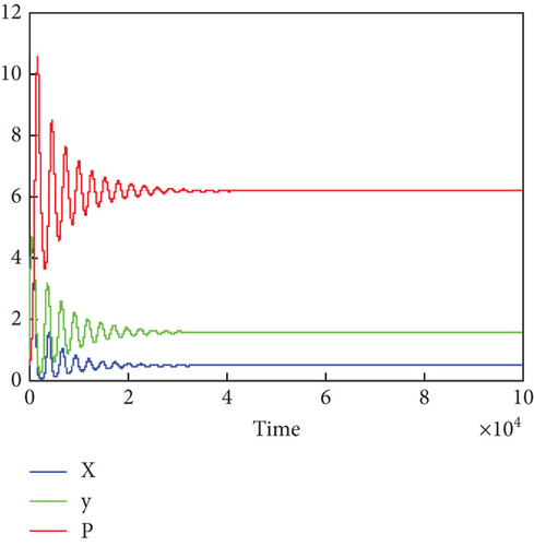
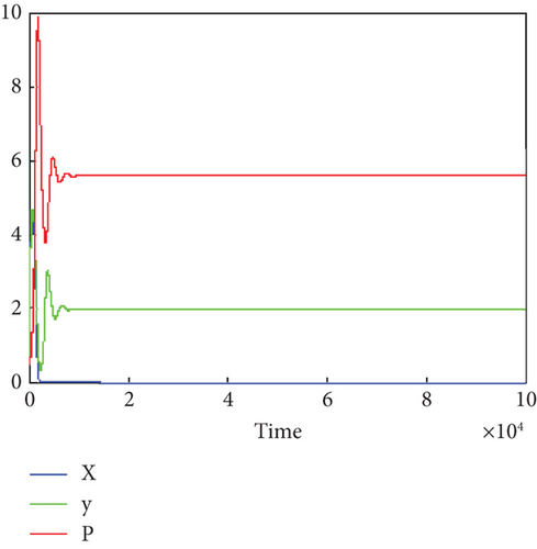
When we increase the value of f₁ to 0.3 and fix other parameter values as given in (21), the trajectories of System (1) approach the prey X–free steady state, as shown in Figure 2.

Now, let us increase the value of f₂ to 0.4, and fix other parameter values as given in (21); the trajectories of System (1) approach the prey Y–free steady state, and this is illustrated in Figure 3.

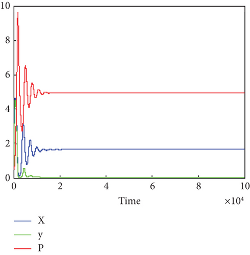
Note that the parameter values used to draw Figures 2 and 3 satisfy the criteria for stability conditions for prey X–free steady state and prey Y–free steady state S₅, respectively, and this confirms the analytical result regarding stability of S₅ and S₆.

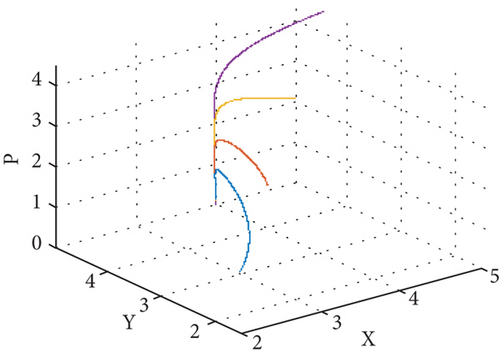
From Figure 1, it is observed that for a small value of fear level, the coexistence of all the populations is guaranteed.

From Figures 2 and 3, it is observed that for a larger value of fear level, no longer in existence of prey species may happen.

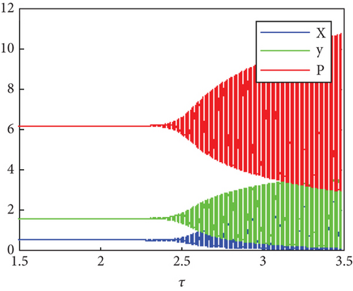
According to time delay, the long-term behavior for a range of value of time delay is plotted in the following bifurcation diagrams, where the x-axis is the range of time delay and the y-axis is limit sets of populations.

In Figure 4, System (1) is solved with τ ∈ [1.5, 3.5 ] and the parameter values are fixed as given in (21). The figure indicates the emergence of Hopf bifurcations near S₇ as, parameter τ passes through .

In Figure 5, System (1) is solved with τ ∈ [5.5, 7.5 ] and f₁ = 0.3 and fixed other parameter values as given in (21); the figure indicates the emergence of Hopf bifurcations near S₆ as τ passes through .

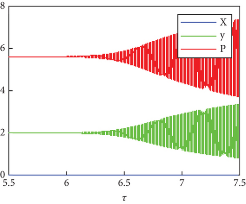
In Figure 6, System (1) is solved with τ ∈ [5.5, 7.5 ] and f₁ = 0.4 and fixed other parameter values as given in (21); the figure indicates the emergence of Hopf bifurcations near S₅ as τ passes through τ ≈ 4.3.

Again, let us choose the parameter values that are given by (22); with those parameter values, the ecological basic reproduction number R_e is less than one. System (1) with parameter values in (22) stabilizes at the predator-free steady state, and this is illustrated in Figure 7(a).

(22)

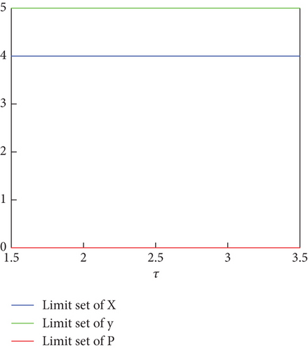
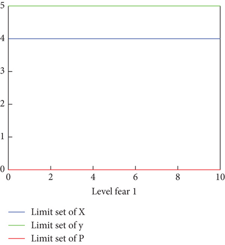
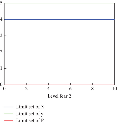
Note that when we vary the value of fear effect and time delay, the value R_e does not change and dynamics near the predator free steady state does not affect and this is illustrated in Figures 7(b) and 7(c). This confirms the analytical result regarding the ecological reproduction number.

7. Conclusion and Discussion

Fears from predators may reduce the reproduction of prey population, and the period of time between the prey predation and predator response to the predation plays a vital role in population. In this paper, the dynamic interaction between two prey species and one predator species under the consideration of the fear effect on both prey species and time delay corresponding to the gestation period is modeled through a set of differential equations. It is explored that System (1) has at most seven steady states; they are denoted by S_i, i = 1, 2, 3, 4, 5, 6,7; it is proved that S₁, S₂, and S₃ are unstable while the criteria for the LAS of the other steady state are determined. The bifurcating values of time delay for occurrence of Hopf bifurcation in System (1) near the prey X–free and prey Y–free steady states are given in Theorem 3 and Theorem 4, respectively. Therefore in Theorems 3 and 4, we can implicate that if the value of time delay is changed, System (1) may induce a transition from the stability situation to the state where the populations oscillate periodically and numerically; this implication is illustrated in Figures 4, 5, and 6. In Figures 1, 2, and 3, we observed that for small value of fear level, the coexistence of all the populations is guaranteed but for larger value of fear level, no longer in existence of prey species may happen. The ecological reproduction R_e for System (1) is also found. It is noted that R_e is independent on the fear level and time delay. By numerical simulation, we have shown that R_e is not affected by change in the value of fear level or time delay as shown in Figure 7. Those analytical and numerical results regarding R_e confirm that the locally stabilization at predator-free steady state is independent of the factors of both fear and time delay.

Conflicts of Interest

The authors declare no conflicts of interest.

Author Contributions

We confirm that the manuscript has been read and approved by all named authors and that there are no other persons who satisfied the criteria for authorship but are not listed. We further confirm that the order of authors listed in the manuscript has been approved by all of us.

Funding

We confirm that the manuscript received no external funding.

Open Research

Data Availability Statement

We confirm the data that support the findings of the manuscript are available on request from the corresponding author.

References

1 Vinoth S., Vadivel R., Nien-Tsu H., Chen C.-S., and Gunasekaran N., Bifurcation analysis in a harvested modified Leslie–Gower model incorporated with the fear factor and prey refuge, Mathematics. (2023) 11, no. 14, https://doi.org/10.3390/math11143118.
10.3390/math11143118
Web of Science® Google Scholar
2 Al-Darabsah I., Tang X., and Yuan Y., A prey-predator model with migrations and delays, Discrete and Continuous Dynamical Systems Series B. (2016) 21, no. 3, 737–761, https://doi.org/10.3934/dcdsb.2016.21.737, 2-s2.0-84959919485.
10.3934/dcdsb.2016.21.737
Web of Science® Google Scholar
3 Elettreby M. F., Two-prey one-predator model, Chaos, Solitons & Fractals. (2009) 39, no. 5, 2018–2027, https://doi.org/10.1016/j.chaos.2007.06.058, 2-s2.0-64049094660.
10.1016/j.chaos.2007.06.058
Web of Science® Google Scholar
4 Arif G. E., Alebraheem J., and Yahia W. B., Dynamics of predator-prey model under fluctuation rescue effect, Baghdad Science Journal. (2023) 20, 1742–1750, https://doi.org/10.21123/bsj.2023.
10.21123/bsj.2023
Web of Science® Google Scholar
5 Mondal C., Dipak K., and Mukherjee D., Bifurcation and global stability of a discrete prey–predator model with saturated prey refuge, Mathematical Methods in the Applied Sciences. (2023) 46, no. 17, 18354–18374, https://doi.org/10.1002/mma.9562.
10.1002/mma.9562
Web of Science® Google Scholar
6 Fatah S., Mustafa A., and Shilan A., Predator and n-classes-of-prey model incorporating Extended Holling type II functional response for n different prey species, AIMS Mathematics. (2022) 8, no. 3, 5779–5788, https://doi.org/10.3934/math.2023291.
10.3934/math.2023291
Google Scholar
7 Holling C. S., Some characteristics of simple types of predation and parasitism, Canadian Entomologist. (1959) 91, no. 7, 385–398, https://doi.org/10.4039/Ent91385-7, 2-s2.0-84880026161.
10.4039/Ent91385-7
Google Scholar
8 Molla H., Rahman M. S., and Sarwardi S., Dynamics of a predator-prey model with Holling type II functional response incorporating a prey refuge depending on both the species, International Journal of Nonlinear Sciences and Numerical Simulation. (2019) 20, no. 1, 89–104, https://doi.org/10.1515/ijnsns-2017-0224, 2-s2.0-85057616676.
10.1515/ijnsns-2017-0224
Web of Science® Google Scholar
9 He M. and Li Z., Stability of a fear effect predator–prey model with mutual interference or group defense, Journal of Biological Dynamics. (2022) 16, no. 1, 480–498, https://doi.org/10.1080/17513758.2022.2091800.
10.1080/17513758.2022.2091800
PubMed Web of Science® Google Scholar
10 Hallam T. G. and Clark C. E., Non-autonomous logistic equations as models of populations in a deteriorating environment, Journal of Theoretical Biology. (1981) 93, no. 2, 303–311, https://doi.org/10.1016/0022-5193(81)90106-5, 2-s2.0-0019845154.
10.1016/0022-5193(81)90106-5
Web of Science® Google Scholar
11 Naji R. K. and Mustafa A. N., The dynamics of an eco-epidemiological model with nonlinear incidence rate, Journal of Applied Mathematics. (2012) 2012, no. 1, 852631, https://doi.org/10.1155/2012/852631, 2-s2.0-84868678282.
10.1155/2012/852631
Google Scholar
12 Hassan K., Mustafa A., and Hama M., An eco-epidemiological model incorporating harvesting factors, Symmetry. (2021) 13, no. 11, https://doi.org/10.3390/sym13112179.
10.3390/sym13112179
Web of Science® Google Scholar
13 Zanette L. Y., White A. F., Allen M. C., and Clinchy M., Perceived predation risk reduces the number of offspring songbirds produce per year, Science. (2011) 334, no. 6061, 1398–1401, https://doi.org/10.1126/science.1210908, 2-s2.0-83255164813.
10.1126/science.1210908
CAS PubMed Web of Science® Google Scholar
14 Wang X., Zanette L., and Xinfu Z. X., Modeling the fear effect in predator-prey interactions, Journal of Mathematical Biology. (2016) 73, no. 5, 1179–1204, https://doi.org/10.1007/s00285-016-0989-1, 2-s2.0-84961843555.
10.1007/s00285-016-0989-1
PubMed Web of Science® Google Scholar
15 Pal S., Pal N., Samanta S., and Chattopadhyay J., Effect of hunting cooperation and fear in a predator-prey model, Ecological Complexity. (2019) 39, 100770, https://doi.org/10.1016/j.ecocom.2019.100770, 2-s2.0-85067917048.
10.1016/j.ecocom.2019.100770
Web of Science® Google Scholar
16 Zhang H., Cay Y., Fu S., and Wang W., Impact of the fear effect in a prey-predator model incorporating a prey refuge, Applied Mathematics and Computation. (2019) 356, 328–337, https://doi.org/10.1016/j.amc.2019.03.034, 2-s2.0-85063610028.
10.1016/j.amc.2019.03.034
Web of Science® Google Scholar
17 Pingping G., Meng F., and Zou X., Dynamics of a three-species food chain model with fear effect, Communications in Nonlinear Science and Numerical Simulation. (2021) 9, 105809, https://doi.org/10.1016/j.cnsns.2021.105809.
10.1016/j.cnsns.2021.105809
Google Scholar
18 Yiping T., Yongli C., Ruoxia Y., Maolin H., and Weiming W., Complex dynamics in an eco-epidemiological model with the cost of anti-predator behaviors, Nonlinear Dynamics. (2022) 107, 3127–3141, https://doi.org/10.1007/s11071-021-07133-4.
10.1007/s11071-021-07133-4
Google Scholar
19 Jimil A. R. and Naji R. K., Modeling and analyzing the influence of fear on the harvested modified Leslie Gower model, Baghdad Science Journal. (2023) 20, no. 5, 1701–1712, https://doi.org/10.21123/bsj.2023.ID.
10.21123/bsj.2023.ID
Google Scholar
20 Liu J., Lv P., Baiu L. V., and Zhang T., Dynamics of a predator-prey model with fear effect and time delay, Complexity. (2021) 2021, no. 1, https://doi.org/10.1155/2021/9184193, 9184193.
10.1155/2021/9184193
Web of Science® Google Scholar
21 Haque M., Sarwardi S., Preston S., and Venturino E., Effect of delay in a Lotka Volterra type predator- prey model with a transmissible disease in the predator species, Mathematical Biosciences. (2011) 234, no. 1, 47–57, https://doi.org/10.1016/j.mbs.2011.06.009, 2-s2.0-80054120406.
10.1016/j.mbs.2011.06.009
PubMed Web of Science® Google Scholar
22 Abbas Z. S. and Naji R. K., Modeling and analysis of the influence of fear on a harvested food web system, Mathematics. (2022) 10, no. 18, https://doi.org/10.3390/math10183300.
10.3390/math10183300
Web of Science® Google Scholar
23 Naji R. K. and Majeed S. J., The dynamical analysis of a delayed prey-predator model with a refuge-stage structure prey population, Journal of Mathematical and Informatics Sciences. (2020) 15, no. 1, 135–159, https://ijmsi.ir/article-1-1116-en.pdf.
10.29252/ijmsi.15.1.135
Web of Science® Google Scholar
24 Lavanya R., Vinth S., Sathiyanathan K., Zeric N. T., Hammachukiatkul P., and Vadivel R., Dynamical behavior of a delayed Holling type-II predator prey model with predator cannibalism, Journal of Mathematics. (2022) 2022, no. 1, 4071375, https://doi.org/10.1155/2022/4071375.
10.1155/2022/4071375
Web of Science® Google Scholar
25 Alsakaji H. J., Kundu S., and Rihan F. A., Delay differential model of one-predator two-prey system with Monod-Haldane and Holling type II functional responses, Applied Mathematics and Computation. (2020) 397, 125919, https://doi.org/10.1016/j.amc.2020.125919.
10.1016/j.amc.2020.125919
Google Scholar
26 Rihan F. A., Alsakaji H. J., and Rajivganthi C., Stability and Hopf bifurcation of three-species prey-predator system with time delays and Allee effect, Complexity. (2020) 2020, https://doi.org/10.1155/2020/7306412, 7306412.
10.1155/2020/7306412
Web of Science® Google Scholar
27 Belew B. and Melese D., Modeling and analysis of predator-prey model with fear effect in prey and hunting cooperation among predators and harvesting, Journal of Applied Mathematics. (2022) 2022, no. 1, https://doi.org/10.1155/2022/2776698, 2776698.
10.1155/2022/2776698
Web of Science® Google Scholar

Citing Literature

All articles

Dynamical Analysis of a Delay Two-Prey–One-Predator Model Incorporating Fear Effect in the Growth Rate of Preys

Abstract

1. Introduction

2. The Mathematical Model and Its Solution Properties

3. Existence of Steady States

4. Local Stability and Hopf Bifurcation

5. The Ecological Basic Reproduction Number

6. Numerical Simulation

7. Conclusion and Discussion

Conflicts of Interest

Author Contributions

Funding

Open Research

Data Availability Statement

References

Citing Literature

Figures

References

Information

About Wiley Online Library

Help & Support

Opportunities

Connect with Wiley

Dynamical Analysis of a Delay Two-Prey–One-Predator Model Incorporating Fear Effect in the Growth Rate of Preys

Abstract

1. Introduction

2. The Mathematical Model and Its Solution Properties

3. Existence of Steady States

4. Local Stability and Hopf Bifurcation

5. The Ecological Basic Reproduction Number

6. Numerical Simulation

7. Conclusion and Discussion

Conflicts of Interest

Author Contributions

Funding

Open Research

Data Availability Statement

References

Citing Literature

Figures

References

Related

Information