Improving the Generalization and Robustness of Computer-Generated Image Detection Based on Contrastive Learning
Abstract
With the rapid development of image generation techniques, it becomes much more difficult to distinguish high-quality computer-generated (CG) images from photographic (PG) images, challenging the authenticity and credibility of digital images. Therefore, distinguishing CG images from PG images has become an important research problem in image forensics, and it is crucial to develop reliable methods to detect CG images in practical scenarios. In this paper, we proposed a forensics contrastive learning (FCL) framework to adaptively learn intrinsic forensics features for the general and robust detection of CG images. The data augmentation module is specially designed for CG image forensics, which reduces the interference of forensic-irrelevant information and enhances discrimination features between CG and PG images in both the spatial and frequency domains. Instance-wise contrastive loss and patch-wise contrastive loss are simultaneously applied to capture critical discrepancies between CG and PG images from global and local views. Extensive experiments on different public datasets and common postprocessing operations demonstrate that our approach can achieve significantly better generalization and robustness than the state-of-the-art approaches. This manuscript was submitted as a pre-print in the following link https://papers.ssrn.com/-sol3/papers.cfm?abstract_id=4778441.
1. Introduction
Over the past decade, the rapid development of multimedia generation techniques has enabled people to easily create computer-generated (CG) images with high quality. Computer graphics techniques such as three-dimensional (3D) modeling and rendering have been extensively used to generate photorealistic CG images. With the advances in AI-based generation techniques such as generative adversarial networks (GANs), high-resolution CG images can be synthesized automatically with less human intervention. These high-quality CG images tend to be indistinguishable from photographic (PG) images by human naked eyes and may be abused by malicious users to create deceptive content and spread false information, leading to severe trust and security concerns. Therefore, it is crucial to develop reliable methods to distinguish CG images from PG images in practical scenarios. Some previous works are proposed to differentiate between CG and PG images via manually extracting discriminative features in the spatial domain [1–3] or frequency domain [4–6]. Constructing these hand-crafted features is time-consuming and heavily requires human prior knowledge, leading to limited detection performance, especially for complex and challenging datasets. In recent years, deep neural networks, such as convolutional neural networks (CNNs), have witnessed huge successes in the field of image forensics due to their strong capability of representation learning. There have been a growing number of CNN-based methods proposed for CG image detection by designing CNNs to reveal the trace left by the computer generation process. Some discriminative features (e.g., statistical properties of spatial domain [7, 8], channel and pixel correlation [9], texture information [10], gradient information [11], and noise information [12–14]) are explored to improve forensic performance.
Despite advances in designing CNNs for the detection of CG images, extra domain knowledge and experience are often required, and only one or two specific traces of computer generation are concerned. With the continuous development of computer generation techniques, these specific artifacts may be weakened, leading to reduced detection performance. In addition, these works treat CG image detection as a binary classification problem, and the CNNs are trained by supervision of the cross-entropy (CE) loss. The common CE-based classification framework tends to learn the features that inevitably depend on the distribution of training data. Thus, it remains a challenge to drive CNNs to learn intrinsic forensic features that are data-independent and reflect differences between CG and PG images. Consequently, the existing CNN-based methods suffer from performance limitations which mainly include (a) generalization on unseen datasets and unseen computer generation techniques and (b) robustness against various postprocessing operations. Therefore, it is desirable to develop a new framework that can adaptively learn intrinsic forensic features to achieve general and robust detection of CG images.
- •
Instead of designing CNNs that focus on some specific distinct features of CG and PG images, we proposed a contrastive learning framework to adaptively learn intrinsic forensic features for the general and robust detection of CG images
- •
The data augmentation module is specially designed for CG image forensics, which reduces the interference of image content and enhances the learning of forensic-related features in both the spatial and frequency domains
- •
A comprehensive supervised contrastive loss, which consists of instance-wise contrastive loss and patch-wise contrastive loss, is applied to capture globally and locally correlated discrepancies between CG and PG images
- •
Experimental results demonstrate that our method achieves significantly better performance on CG image detection than the state-of-the-art methods, especially in terms of generalization and robustness
The rest of this paper is organized as follows. In Section 2, we reviewed the deep learning–based approaches for the detection of CG images and contrastive learning. Section 3 presents the proposed contrastive learning framework for the detection of CG images. Experimental results are reported in Section 4. The visualization analysis is shown in Section 5. Finally, the concluding remarks are given in Section 6.
2. Related Work
2.1. CNN-Based CG Image Detection
In recent years, deep learning–based methods have gradually played a more important role in image forensics research than traditional methods based on hand-crafted features. A growing number of CNN-based methods have been developed to address CG image forensics. Previous CNN-based methods rarely deviate from a local-to-global manner [7–9, 12, 13, 16, 17]. CNNs are applied to obtain local decisions on a certain number of image patches that are cropped from a full-size image, and a global decision can be obtained via a majority vote scheme. Therefore, the performance improvement of these methods may come at the cost of high computational overhead.
More recently, CNN-based methods have been developed for CG image forensics based on an entire image or image patch, and the detection performances are improved by designing network frameworks to explore effective distinct features between CG and PG images. Several studies [14, 18] have developed dual-branch networks to learn RGB-based distinct features and high frequency–based distinct features of CG and PG images simultaneously. Bai et al. [10] designed a texture-aware network to perform texture enhancement on features and learn the relations of different feature channels. Furthermore, considering the existing datasets of CG image forensics being constructed in former times and limited in both quantity and diversity, they built a new complex and diverse benchmark for the CG forensics task, i.e., a large-scale CG images benchmark (LSCGB). Gangan et al. [19] explored discriminative features in different color spaces, RGB, LCH, and HSV by parallelly fusing three EfficientNet networks [20].
Yao et al. [21] proposed a CG image detection method by extracting both the shallow and the deep semantic features of the image which are beneficial to the task of CG image forensics. Ju et al. [22] proposed a global and local feature fusion (GLFF) framework to learn multiscale global features and refined local features for detecting AI-generated images.
Existing deep learning–based methods have demonstrated promising performance in CG image forensics, but their generalization capability and robustness remain limited. This is because designing effective network architectures for CG image detection often requires extensive domain knowledge and experience. In addition, these methods typically focus on specific discrepancies between CG and PG images. Moreover, these existing CNNs used for CG image detection are trained only by the supervision of CE loss, leading to insufficient learning of intrinsic forensic features. In this work, we proposed a supervised contrastive learning framework for CG image forensics to adaptively learn intrinsic forensic features and further achieve high generalization capability and robustness.
2.2. Contrastive Learning
Contrastive learning has come to researchers’ notice in recent years because of its philosophy of maximizing the mutual information between two transformation views of the same image [23]. The transformation views contribute to learning transformation invariant features that can resist perturbations [24]. The traditional contrastive learning works [25–28] primarily employed self-supervised pretraining by designing pretext tasks, and the pretrained models were able to achieve good performance when fine-tuned on downstream tasks. Promising transfer ability on downstream tasks fully demonstrates its efficiency in learning general representation.
Khosla et al. [29] first conducted research on supervised contrastive learning in tasks such as detection, classification, and segmentation, demonstrating that models trained end-to-end with supervised contrastive learning outperformed unsupervised pretrained models that were fine-tuned on specific downstream tasks. Consequently, researchers [30, 31] applied supervised contrastive learning in the deepfake forensics task. Compared to the models solely based on CE loss, the proposed InfoNCE loss has proven to be beneficial in learning the general discriminative features. In addition, recent advancements in image tampering detection [32–34] have showcased that contrastive learning facilitated learning intrinsic features, which emphasize the dissimilarity between authentic and manipulated regions. By leveraging the relationships of local features between tampered and authentic regions for discriminative representation learning, the performance of image tampering detection can be highly improved even in the presence of disturbance. The recent CG image detection work [35] has introduced self-supervised learning by designing pretext tasks. However, there was still a performance gap when compared with a state-of-the-art fully supervised method.
Previous contrastive learning–based works were mostly aimed at image tampering detection or deepfake detection, which may not be suitable for CG image forensics tasks. Based on this, we designed a FCL framework. First, we designed a FAM to extract spatial and frequency domain features that are more conducive to forensics. Subsequently, we applied supervision to the deep and shallow layers of the backbone network to comprehensively learn the inconsistencies between CG and PG images from both global and local perspectives.
3. Methodology
In this section, we begin by detailing the FAM in Section 3.1. Then, in Section 3.2, we present the architecture of our FCL framework. Sections 3.3 and 3.4 are dedicated to patch-wise contrastive learning (PCL) and instance-wise contrastive learning (ICL), respectively. In Section 3.5, we presented the overall optimization function employed in our method.
3.1. FAM
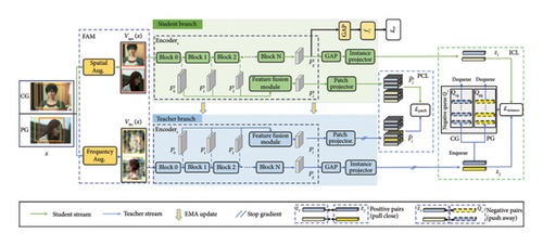
In our FCL framework, data augmentation plays a vital role in capturing general forensic cues. Our specially designed FAM serves the purpose of eliminating task-irrelevant factors within training samples and uncovering more discriminative information from both spatial and frequency domains. As depicted in Figure 1, we obtained two different views of the original image via random cropping. These views are then subjected to spatial or frequency augmentation to generate the inputs for contrastive learning.
3.1.1. Spatial Augmentation
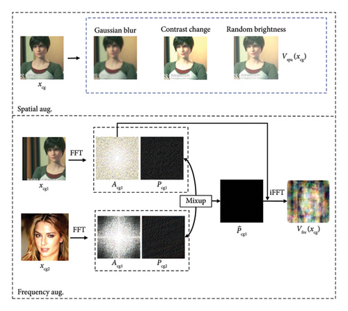
In general, certain manipulation traces belong to method-specific forensic cues (i.e., noncritical cues), which can potentially hinder the detector’s generalization ability when decisions heavily rely on this biased information. The previous work [36] demonstrated the disparities between CG and PG images in different color spaces. Nevertheless, since each generation model possesses unique spatial statistics, it becomes challenging to detect unknown CG images through these forensic cues. Given this observation, we mitigated the influence of spatial statistical features through several global image operations, including Gaussian Blur (GB), Random Brightness (RB), and Contrast Change (CC). These spatial augmentations modify the spatial statistics, thereby preventing the detector from overfitting to spatial data-specific features that may not generalize effectively.
3.1.2. Frequency Augmentation
Figure 2 gives the pipeline of our proposed FAM. By applying spatial and frequency augmentation in different branches, the positive pair (Vspa(x), Vfre(x)) exhibits different high-level semantic content but still shares similar amplitude spectrum information. By pulling close the distance between the spatial and frequency views of the same image, the model can effectively learn more critical forensics information to boost its generalization performance.
3.2. Pipeline of FCL Framework
3.3. PCL Module
Since it is still challenging to replicate the complex textures found in real-world photographs [10] in the process of CG image generation, local artifacts are considered as evident forensics clues. Previous works have demonstrated that more texture features exist in shallow layers [40, 41]. Motivated by these findings, we first proposed the feature fusion module (FFM) to obtain local feature representations from shallow layers and then learn discriminative information through our proposed PCL.
In FFM, the shallow features from the first three downsampling blocks denoted as (where layer = 0, 1, 2) are separately encoded into the latent space with the same spatial size as . These embeddings are concatenated together and further transformed into a low-dimensional embedding through the patch projector (consisting of two 1 × 1 convolutional layers). Note that c is the spatial size of the local feature embedding, and h is the channel dimension. We denoted the vector at each spatial location in and as query embedding qi and key embedding ki, where i, j = 1, 2, …, c2. In this way, each embedding represents the local feature corresponding to the respective spatial location.
3.4. ICL Module
The instance-wise contrastive loss effectively enhances the invariance between the spatial and frequency augmented views of a single input, simultaneously enlarging the difference between the augmented views of different categories. Consequently, the model can effectively learn more generalized knowledge compared with the CE-based models.
3.5. Overall Loss Function
4. Experiment
4.1. Datasets
-
Columbia [42]: The dataset is one of the most commonly used datasets in CG image forensics benchmarking. It comprises 1600 CG images generated by graphical software tools such as 3 ds MAX, Softimage-XSI, Maya, Terragen, and others, as detailed in [42]. In addition, 1600 PG images have been primarily sourced from Google Image Search and personal collections.
-
Tokuda [43]: This dataset comprises 4850 CG and 4850 PG images with a large diversity of image content and quality. All images in this dataset are collected from the Internet. The CG images are generated by computer graphics method and photorealistic. The PG images are captured by various devices, and both indoor and outdoor landscapes are included.
-
Rahmouni [7]: This dataset contains 1800 CG and 1800 PG images, among which the CG images are from screenshots of 3D games selected from the Level-Design Reference dataset, and the PG images are collected from raw dataset RAISE [45].
-
SPL2018 [44]: This dataset is composed of 6800 PG and 6800 CG images. The CG images are generated by more than 50 graphical software tools such as Maya and 3DS Max. The PG images are captured under various environmental conditions with different camera models. It is worth noting that the images of the dataset have diverse contents and a wide range of image resolutions.
-
LSCGB [10]: This is a challenging benchmark for CG image forensics because of the large scale and high diversity. It contains 71,168 CG and 71,168 PG images, which are orders of magnitude bigger than the above existing CG datasets. The CG images are sourced from four different scenes, i.e., games, movies, models, and GANs. In the first three sources, the CG images are created by different computer graphics techniques. Notably, various GAN techniques are introduced to provide more CG images, which are not considered in other existing CG image datasets. The PG images are varied in terms of image content, camera models, and photographer styles.
We followed the implementation details in [10]. All five datasets were separated into train, valid, and test datasets with a ratio of 7:1:2.
4.2. Experimental Settings
In our experiments, we followed the preprocessing strategy proposed in [10]. During training, we randomly cropped the images with a size of 224 × 224. We also used a class-balanced random sampler to balance the distribution of CG and PG images within each training batch. Each of the three spatial augmentations is conducted with a 50% probability. During evaluation, we centrally cropped the images with a size of 224 × 224 with no augmentation.
Our method is implemented with PyTorch library on two NVIDIA GTX 3090 GPU cards. EfficientNet-B4 (EN-B4) [20] pretrained on the ImageNet [46] is used as our backbone. The model is optimized by Adam with an initial learning rate of 1 × 10⁻³, a weight decay of 1 × 10⁻⁵, and a batchsize of 32. The total training epoch number is 30, and the learning rate decays by 0.4 every 5 epochs. According to the experience of the previous work [25], the hyperparameter α is set as 0.999, and the temperature parameter τ is set to 0.07. β is randomly selected from a uniform distribution between 0 and 1. The dimensions d and h are both set to 128, and the final feature map size c is set to 7. The number of negative samples K is set to 30,000. Following the previous work [10], we mainly use Accuracy (ACC) as the evaluation metric.
4.3. Intradataset Evaluation
We initially conducted a comparative analysis between our proposed FCL and state-of-the-art CG image detection algorithms within the same intradataset setting. The results are shown in Table 1, where the best results are highlighted in bold. On the whole, our FCL method demonstrates promising performance across the five datasets and achieves a certain improvement compared to other methods. Notably, when fairly evaluated on the recent dataset LSCGB, it exhibits a significant improvement from 91.45% to 95.11% compared to the best method (i.e., Bai et al. [10]). The excellent detection performance of FCL can be attributed to the designed data augmentation module and the comprehensive contrastive loss, which enables the detector to capture critical discrepancies between CG and PG images. On the other hand, we observed that the performance of our FCL is slightly lower than the second best method (i.e., Bai et al. [10]) in the case of Rahmouni et al. [7] and Columbia [42] datasets. However, in the following generalization and robustness evaluations, our FCL achieves much better performance. This demonstrates that the proposed method tends to learn intrinsic forensic features so that it does not easily overfit on small datasets.
| Dataset ⟶Methods ↓ | Rahmouni [7] | Columbia [42] | Tokuda [43] | SPL2018 [44] | LSCGB [10] | Average |
|---|---|---|---|---|---|---|
| Rahmouni [7] | 85.16 ± 0.23 | 78.19 ± 0.20 | 82.75 ± 0.34 | 82.17 ± 0.15 | 77.45 ± 0.27 | 81.14 |
| Chawla [12] | 94.46 ± 0.09 | 85.81 ± 0.45 | 85.11 ± 0.30 | 90.82 ± 0.18 | 77.12 ± 0.36 | 86.67 |
| Quan [16] | 90.49 ± 0.13 | 89.99 ± 0.17 | 88.31 ± 0.17 | 88.61 ± 0.08 | 82.80 ± 0.13 | 88.04 |
| Yao [13] | 92.93 ± 0.10 | 88.01 ± 0.19 | 85.52 ± 0.18 | 83.11 ± 0.21 | 82.91 ± 0.18 | 86.50 |
| Meena [14] | 99.70 ± 0.12 | 92.98 ± 0.18 | 93.65 ± 0.12 | 95.43 ± 0.23 | 90.09 ± 0.19 | 94.37 |
| Nguyen [8] | 99.71 ± 0.09 | 94.91 ± 0.13 | 94.42 ± 0.11 | 96.38 ± 0.20 | 90.02 ± 0.07 | 95.09 |
| Huang [17] | 99.56 ± 0.17 | 91.32 ± 0.08 | 94.24 ± 0.16 | 95.66 ± 0.13 | 90.18 ± 0.18 | 94.19 |
| Zhang [9] | 99.72 ± 0.09 | 91.26 ± 0.26 | 92.04 ± 0.06 | 95.33 ± 0.19 | 90.42 ± 0.15 | 93.75 |
| Bai [10] | 99.94 ± 0.06 | 97.76 ± 0.15 | 96.35 ± 0.14 | 96.89 ± 0.10 | 91.45 ± 0.08 | 96.48 |
| Ours | 99.30 ± 0.31 | 95.68 ± 0.75 | 96.98 ± 0.13 | 97.49 ± 0.21 | 95.11 ± 0.91 | 96.91 |
- Note: Comparative results for state-of-the-art methods on five CG image datasets in terms of ACC (%). The best results are highlighted in bold.
4.4. Generalization Ability Experiments
The generalization ability of models is important in real-world practical applications. To demonstrate the generalization of our proposed FCL, we conducted cross-dataset evaluations. Specifically, the models are trained on the LSCGB and evaluated on the other four datasets, i.e., SPL2018 [44], Columbia [42], Rahmouni [7], and Tokuda [43].
The experimental results in terms of ACC (%) are illustrated in Table 2. Generally speaking, all the detectors experience performance degradation under cross-dataset evaluation. Compared with prior deep learning–based arts, our method has the least decrease in detection accuracy. Especially on the Rahmouni et al.’s [7] dataset, the second best method (i.e., Bai et al. [10]) experiences a decrease of 15.57%, while our method decreases only 7.26%. On the SPL2018 [44] and Columbia [42] datasets, the performance degradation of our method is 3.36% and 4.35%, respectively, which is smaller than other state-of-the-art methods. To evaluate the performance of the proposed model comprehensively, we adopted additional evaluation metrics including recall, area under the curve (AUC), and equal error rate (EER) and compared the performance with three state-of-the-art methods. The comparison results are obtained by training the models with their official public codes on our training samples. The results in terms of recall (%), AUC (%), and EER (%) are illustrated in Tables 3, 4, and 5, respectively. Our model achieved the best performance under all evaluation metrics. The proposed FCL outperforms Bai et al. [10] with average recall and AUC improvements of 8.68% and 2.87%, respectively. The average EER of FCL is 13.16% lower than that of Bai et al. [10]. This result shows that our proposed FCL framework takes advantage of more critical discriminate discrepancies between CG and PG images, which generally exist in different datasets. This mainly benefits from our designed framework which is proficient in learning a more general feature representation.
Dataset ⟶ Methods ↓ |
LSCGB | Testing | ||||
|---|---|---|---|---|---|---|
| SPL2018 [44] | Columbia [42] | Rahmouni [7] | Tokuda [43] | Average | ||
| Nguyen [8] | 90.02 ± 0.07 | 62.15 ± 1.56 | 78.24 ± 2.65 | 72.11 ± 2.32 | 78.71 ± 1.95 | 72.80 |
| Huang [17] | 90.18 ± 0.18 | 74.59 ± 1.79 | 78.96 ± 1.26 | 65.13 ± 2.29 | 80.78 ± 1.67 | 74.87 |
| Zhang [9] | 90.42 ± 0.15 | 80.56 ± 1.32 | 68.86 ± 2.06 | 54.30 ± 3.26 | 72.57 ± 2.14 | 69.07 |
| VGG-19 [47] | 89.48 ± 0.13 | 78.10 ± 1.13 | 77.04 ± 1.61 | 67.36 ± 1.72 | 77.16 ± 1.39 | 74.92 |
| Bai [10] | 91.45 ± 0.08 | 85.32 ± 0.93 | 81.07 ± 1.77 | 75.88 ± 1.97 | 83.95 ± 0.65 | 81.56 |
| Yao [21] | 91.26 ± 0.17 | 82.35 ± 0.83 | 70.14 ± 1.34 | 75.39 ± 1.69 | 90.91 ± 0.59 | 79.70 |
| Gangan [19] | 90.56 ± 0.11 | 77.41 ± 0.92 | 73.49 ± 1.65 | 69.42 ± 1.74 | 87.45 ± 0.85 | 76.94 |
| Ours | 95.11 ± 0.19 | 91.75 ± 0.43 | 90.76 ± 0.98 | 87.85 ± 0.69 | 96.79 ± 0.33 | 91.79 |
- Note: Cross-dataset evaluation from LSCGB to four unseen datasets in terms of ACC (%). The best results are highlighted in bold.
Dataset ⟶ Methods ↓ |
SPL2018 [44] | Columbia [42] | Rahmouni [7] | Tokuda [43] | Average |
|---|---|---|---|---|---|
| Bai [10] | 86.40 ± 0.65 | 83.23 ± 1.20 | 60.34 ± 1.59 | 89.33 ± 0.32 | 79.83 |
| Yao [21] | 89.91 ± 0.51 | 88.59 ± 1.04 | 55.96 ± 1.42 | 90.98 ± 0.45 | 81.36 |
| Gangan [19] | 84.77 ± 1.25 | 87.25 ± 1.17 | 58.36 ± 1.30 | 91.05 ± 0.63 | 80.36 |
| Ours | 96.40 ± 0.42 | 98.24 ± 0.68 | 61.75 ± 0.66 | 97.63 ± 0.28 | 88.51 |
- Note: The best results are highlighted in bold.
Dataset ⟶ Methods ↓ |
SPL2018 [44] | Columbia [42] | Rahmouni [7] | Tokuda [43] | Average |
|---|---|---|---|---|---|
| Bai [10] | 93.24 ± 0.15 | 93.76 ± 0.52 | 94.63 ± 0.39 | 94.40 ± 0.11 | 94.01 |
| Yao [21] | 92.56 ± 0.16 | 95.21 ± 0.28 | 93.40 ± 0.29 | 96.55 ± 0.11 | 94.43 |
| Gangan [19] | 91.05 ± 0.21 | 94.28 ± 0.64 | 92.79 ± 0.51 | 95.21 ± 0.38 | 93.33 |
| Ours | 96.70 ± 0.10 | 95.81 ± 0.36 | 95.77 ± 0.30 | 99.22 ± 0.12 | 96.88 |
- Note: The best results are highlighted in bold.
Dataset ⟶ Methods ↓ |
SPL2018 [44] | Columbia [42] | Rahmouni [7] | Tokuda [43] | Average |
|---|---|---|---|---|---|
| Bai [10] | 19.96 ± 0.63 | 21.09 ± 0.82 | 27.76 ± 0.91 | 23.40 ± 0.52 | 23.05 |
| Yao [21] | 20.31 ± 0.51 | 29.65 ± 0.60 | 33.42 ± 0.65 | 16.68 ± 0.42 | 25.02 |
| Gangan [19] | 25.56 ± 0.75 | 26.87 ± 0.90 | 30.10 ± 0.99 | 18.45 ± 0.69 | 25.25 |
| Ours | 10.55 ± 0.42 | 7.67 ± 0.67 | 15.78 ± 0.58 | 5.57 ± 0.35 | 9.89 |
- Note: The best results are highlighted in bold.
4.5. Robustness Experiments
In real-world scenarios, postprocessing operations such as compression and resizing may be used for the images transmitted over the Internet, which inevitably affect the performance of the detectors of CG images. Robustness is an essential indicator that reflects the ability of the detectors to resist these interferences in practical applications.
In this subsection, we evaluated the robustness of the proposed FCL against different postprocessing operations and compared our approach with current state-of-the-art methods. The models are all trained and tested on the LSCGB dataset. Following Bai’s experiential setting [10], we considered six image postprocessing operations commonly used in practical scenarios, including JPEG compression (quality factor (QF) = 70), scaling (upscaling 20% or downscaling 20%), median filtering (filter size = 3 × 3), mean filtering (filter size = 3 × 3), and Gaussian noise (zero mean and σ = 1). The testing results are shown in Table 6. Although all studied methods suffer a decline in performance when compared with results without postprocessing operations, our proposed FCL outperforms other state-of-the-art methods in most detection cases.
Dataset ⟶ Methods ↓ |
LSCGB | Testing | ||||||
|---|---|---|---|---|---|---|---|---|
| JPEG (70%) | Up (20%) | Down (20%) | Median (3 × 3) | Mean (3 × 3) | Noise (σ = 1) | Average | ||
| Nguyen [8] | 90.02 ± 0.07 | 76.22 ± 1.59 | 86.16 ± 1.60 | 84.26 ± 1.09 | 71.25 ± 1.25 | 65.81 ± 0.91 | 82.20 ± 0.49 | 77.65 |
| Huang [17] | 90.18 ± 0.18 | 74.35 ± 1.61 | 83.35 ± 0.92 | 83.55 ± 1.00 | 68.26 ± 1.36 | 62.23 ± 1.12 | 83.78 ± 0.59 | 75.92 |
| Zhang [9] | 90.42 ± 0.15 | 70.82 ± 1.52 | 76.16 ± 1.19 | 79.23 ± 1.05 | 67.05 ± 1.45 | 68.43 ± 1.06 | 82.34 ± 0.66 | 74.01 |
| VGG-19 [47] | 89.48 ± 0.13 | 71.05 ± 1.56 | 78.91 ± 1.18 | 78.03 ± 1.19 | 67.15 ± 1.49 | 61.15 ± 1.05 | 78.69 ± 0.79 | 72.50 |
| Bai [10] | 91.45 ± 0.08 | 77.37 ± 1.25 | 89.01 ± 0.89 | 87.76 ± 0.98 | 73.87 ± 1.09 | 67.95 ± 0.94 | 85.76 ± 0.61 | 80.29 |
| Yao [21] | 91.26 ± 0.27 | 75.91 ± 0.55 | 87.78 ± 1.11 | 88.16 ± 1.28 | 70.88 ± 1.02 | 66.39 ± 0.88 | 82.73 ± 1.04 | 78.64 |
| Gangan [19] | 90.56 ± 0.08 | 73.45 ± 1.26 | 85.94 ± 0.69 | 84.32 ± 0.74 | 69.93 ± 1.35 | 62.74 ± 1.53 | 80.17 ± 0.47 | 76.09 |
| Ours | 95.11 ± 0.19 | 80.27 ± 0.38 | 94.16 ± 0.34 | 89.09 ± 0.46 | 88.89 ± 0.29 | 94.52 ± 0.42 | 89.68 ± 1.12 | 89.44 |
- Note: The best results are highlighted in bold.
For instance, the accuracy of the proposed method decreases by 6.22% under median filtering, while the second-best method (i.e., Bai et al. [10]) suffers the decline of 17.58%. When encountering 3 × 3 mean filtering, our method drops 0.59%, while the second-best method (i.e., Zhang et al. [9]) drops 21.99%. This might be explained by the reason that these state-of-the-art methods tend to capture local-level forgery information, which can be readily destroyed by postprocessing operations.
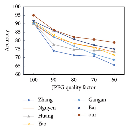
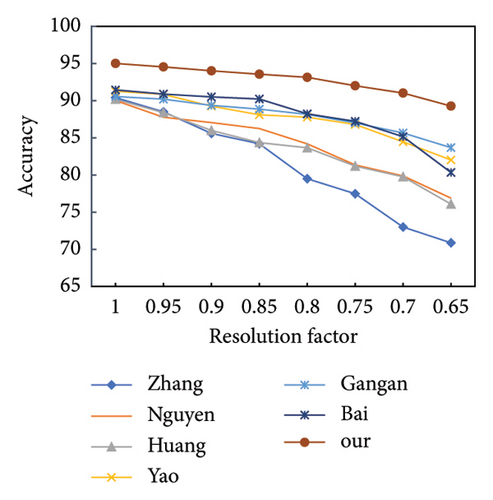
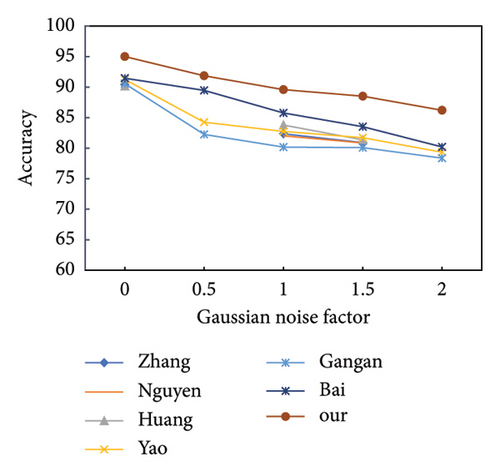
Figure 3 shows the robustness evaluation against JPEG compression, downscale, and Gaussian noise with different parameters. The QF of JPEG compression is set to {90, 80, 70, 60}. The downscale ratio is set from 0.95 to 0.65. The Gaussian noise factor is set from 0.5 to 2. From Figure 3, it can be seen that as the interference intensity increases, the performance of our proposed FCL declines slowly when compared with other state-of-the-art methods. It indicates the superior robustness of our proposed model, especially under a high degree of postprocessing operations. This demonstrates that our proposed framework focuses on more essential distinctive features between CG and PG images. Such essential features are difficult to be affected by common postprocessing operations.
4.6. Ablation Experiments
In this subsection, we conducted ablation experiments to verify the effects of each component in our proposed FCL framework. The variants are all trained on the LSCGB dataset [10] and tested on the SPL2018 [44], Tokuda [43], and Columbia [42] datasets. Since generalization is the most important issue in the CG forensics task, we mainly focused on analyzing the generalization capability of different models.
4.6.1. Effectiveness of Different Proposed Components
We conducted ablation experiments to verify the effectiveness of each component in our proposed FCL. We created the following variations: 1) baseline model (EN-B4 [20]), 2) FCL without FAM, 3) FCL without ICL, 4) FCL without PCL, and 5) our proposed FCL framework.
The quantitative results are shown in Table 7. The comparison between Variation 2 and Variation 5 can demonstrate the effectiveness of our proposed FAM module. For PCL and ICL components, we can observe a certain performance decline in cross-dataset evaluations when any one of them is removed. Specifically, when the PCL module is removed, the ACC result on SPL2018 [44] drops from 91.75% to 89.87%. These findings suggest that our proposed FCL can gain deeper insights into the inherent differences between CG and PG images by combining FAM, ICL, and PCL, thus the detection performance is significantly enhanced.
| SPL2018 [44] | Tokuda [43] | Columbia [42] | |
|---|---|---|---|
| EN-B4 [20] | 87.21 ± 0.47 | 93.77 ± 1.39 | 84.21 ± 1.61 |
| w/o FAM | 88.40 ± 0.48 | 94.74 ± 0.41 | 89.25 ± 0.98 |
| w/o PCL | 89.87 ± 0.32 | 95.21 ± 0.48 | 88.97 ± 1.05 |
| w/o ICL | 89.21 ± 0.27 | 94.69 ± 0.33 | 88.51 ± 1.07 |
| FCL | 91.75 ± 0.43 | 96.79 ± 0.33 | 90.76 ± 0.98 |
- Note: ACC scores (%) are reported. The best results are highlighted in bold.
4.6.2. Impacts of Different Forensics Augmentations
We conducted an ablation experiment to show the impacts of different forensics augmentation strategies. Specifically, we defined the following variations: (1) FCL without spatial and frequency domain augmentation, (2) FCL without GB, (3) FCL without RB, (4) FCL without CC, (5) FCL without spatial domain augmentation, (6) FCL without frequency domain augmentation, and (7) our proposed FCL framework.
From the first row of Table 8, we can directly see that the generalization performance is poor when our proposed FAM is removed. The results of Rows 2–4 of Table 5 show that there is a slight decrease in performance compared to FCL when one of these spatial augmentation operations (GB, RB, or CC) is removed. This indicates that each of these augmentation operations contributes positively to the performance of the model. From the fifth row, it is easily observed that the ACC scores on the three datasets all suffer a decline when the proposed spatial augmentation is removed. In the sixth row, when we remove the proposed Phase Mixup, the ACC scores decrease by 2.71% on SPL2018 [44] and 1.4% on Columbia [42]. This further demonstrates that the high-frequency component contains more forensic-related information. The ablation experiment demonstrates that the application of forensic augmentation is beneficial to improve generalization performance. This further illustrates that the high-frequency component contains more forensic-relevant information. This ablation experiment shows that applying forensic augmentation is critical for increasing generalization performance.
| SPL2018 [44] | Tokuda [43] | Columbia [42] | |
|---|---|---|---|
| w/o FAM | 88.40 ± 0.48 | 94.74 ± 0.41 | 89.25 ± 0.98 |
| w/o GB | 91.09 ± 0.37 | 96.04 ± 0.59 | 89.88 ± 0.61 |
| w/o RB | 91.35 ± 0.44 | 96.20 ± 0.85 | 90.44 ± 1.01 |
| w/o CC | 91.26 ± 0.44 | 96.15 ± 1.02 | 90.30 ± 0.89 |
| w/o spat Aug. | 90.53 ± 0.29 | 95.70 ± 0.52 | 89.47 ± 0.73 |
| w/o freq Aug. | 89.04 ± 0.56 | 95.33 ± 0.62 | 89.36 ± 0.56 |
| FCL | 91.75 ± 0.43 | 96.79 ± 0.33 | 90.76 ± 0.98 |
- Note: ACC scores (%) are reported. The best results are highlighted in bold.
- Abbreviations: CC, contrast change; Freq Aug., frequency augmentation; GB, Gaussian blur; RB, random brightness; Spat Aug., spatial augmentation.
4.6.3. Impacts of Different Backbones
To evaluate the effectiveness of our model in various backbones, we tested the performance by integrating our framework with different CNN-based backbones, including VGG-19 [47], EfficientNet-B0 (EN-B0) [20], and ResNet-50 [48]. For VGG-19, we followed the feature extractor in [8], obtaining local and global feature representations to apply our FCL framework. For ResNet-50, we obtained local feature representation by fusing the features from the first three residual blocks and using the output of the last convolutional layer as the global feature representation. In addition to these classic CNN architectures, we also incorporated vision transformer (ViT) [50] as the backbone and evaluated the performance of integrating the proposed FCL with ViT. As shown in Table 9, our proposed framework helps improve the generalization capability when utilizing various backbones. The average ACC improvements are 2.24%, 6.21%, 2.36%, and 6.53% for VGG-19 [47], EN-b0 [20], ResNet-50 [48], and ViT [50], respectively. The proposed contrast learning framework can effectively learn the similarity of intraclass distribution properties and the difference of interclass distribution properties by comparing sample pairs. As a result, the proposed FCL framework enables the backbones to capture forensic-relevant features, thereby improving their generalization capability. The results demonstrated that our proposed FCL framework is universal for extracting intrinsic discriminative clues and can be flexibly injected into different backbones.
| SPL2018 [44] | Tokuda [43] | Columbia [42] | |
|---|---|---|---|
| EN-B0 [20] | 86.78 ± 0.93 | 91.14 ± 1.56 | 84.10 ± 1.85 |
| EN-B0 + FCL | 89.25 ± 0.76 | 93.24 ± 0.72 | 86.25 ± 1.26 |
| VGG-19 [47] | 78.10 ± 1.13 | 77.16 ± 1.39 | 77.04 ± 1.16 |
| VGG-19 + FCL | 84.52 ± 1.22 | 84.09 ± 0.98 | 82.34 ± 1.17 |
| ResNet-50 [48] | 85.61 ± 0.65 | 92.15 ± 0.92 | 81.86 ± 1.77 |
| ResNet-50 + FCL | 88.22 ± 0.49 | 92.93 ± 0.91 | 85.56 ± 1.35 |
| ViT [50] | 90.46 ± 0.25 | 93.95 ± 0.31 | 84.51 ± 1.17 |
| ViT + FCL | 93.82 ± 0.19 | 97.89 ± 0.29 | 96.80 ± 1.09 |
- Note: ACC scores (%) are reported. The best results are highlighted in bold.
5. Visualization
In this section, we provided visualization of attention maps and feature distributions to more clearly demonstrate the effectiveness of our designed FCL.
5.1. T-SNE Feature Embedding Visualization
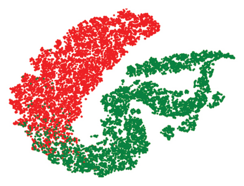
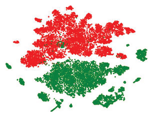
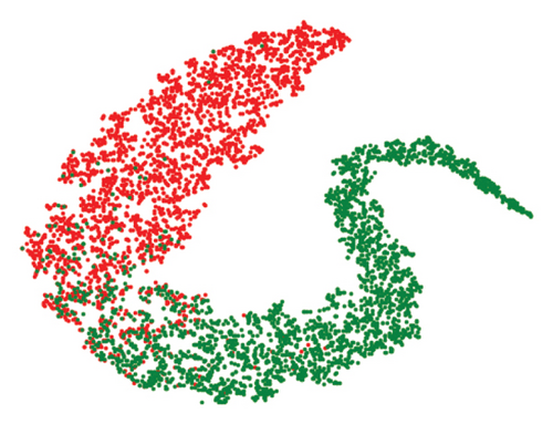
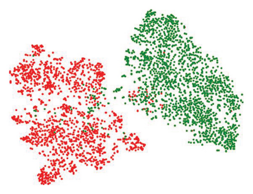
Firstly, we use T-SNE [49] to visualize the feature distribution of the output of our model. As shown in Figure 4, it can be observed that the output feature of the CE-loss–based model has a certain amount of overlap in the training dataset, even if they belong to different categories. Compared with the baseline, our model significantly reduces the overlap area between features of CG and PG images. The same phenomenon is observed on cross-dataset Tokuda, Pedrini, and Rocha [43]. The visualization of the reduced dimensional features further proves our model’s superiority in extracting intrinsic discriminative features.
5.2. Visualization for Detector’s Attention
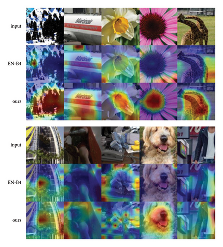
We used the Grad-CAM to visualize the decision regions of the model. As shown in Figure 5, the heatmaps generated by our model highlight different regions for PG and CG images. The first three rows indicate the model’s attention on PG images, and the last three rows indicate the model’s attention on CG images. For PG images, compared with the baseline, our model pays more attention to local texture-complicated areas. For CG images, our model can locate more regions and contain more details where the artifacts exist. This illustrates that our method is efficient in capturing more comprehensive clues than the baseline method by focusing on more extensive areas.
6. Conclusions
In this paper, we proposed a FCL framework for the detection of CG images. A FAM is designed to drive the model to exploit intrinsic forensic-related features in both the spatial and frequency domains. A comprehensive supervised contrastive loss, which consists of instance-wise contrastive loss and patch-wise contrastive loss, is applied to learn essential discrepancies between CG and PG images in both the spatial and frequency domains. Quantitative and qualitative experimental analyses demonstrate a large improvement in the generalization and robustness of our framework. We believed that CG image forensic tasks based on contrastive learning can be further explored in the future research.
In the future, we planned to improve the proposed framework from different aspects. We will explore more feature fusion schemes to further improve forensic performance. In addition, it is valuable to develop an appropriate contrastive learning architecture for the ViT-based backbones. Moreover, the proposed framework will also be extended and modified to tackle more image forensic applications, such as the detection of semantic-focused operations (detecting copy-move, splicing, and inpainting, and the localization of tampered regions).
Conflicts of Interest
The authors declare no conflicts of interest.
Funding
This work was supported in part by the National Natural Science Foundation of China under Grant no. 62102100/62102462, the Basic and Applied Basic Research Foundation of Guangdong Province under Grant no. 2022A1515010108, the Opening Project of Guangdong Provincial Key Laboratory of Information Security Technology under Grant no. 2023B1212060026, Key Research Platforms and Projects of Universities in Guangdong Province Grant no. 2024ZDZX1038, and Research Project of Guangdong Polytechnic Normal University under Grant no. 2021SDKYA127/2022SDKYA027.
Acknowledgments
We would like to thank the authors Bai et al. [10] for kindly sharing the LSCGB dataset and the source code of [10].
Open Research
Data Availability Statement
The data that support the findings of this study are available in LSCGB at https://github.com/wmbai/LSCGB [10].


