Intelligent Recognition for Operation States of Hydroelectric Generating Units Based on Data Fusion and Visualization Analysis
Abstract
This paper proposes a novel recognition approach for operation states of hydroelectric generating units based on data fusion and visualization analysis. First, the principal component analysis (PCA) is employed to simplify signals from multiple channels into a single fused signal, thereby reducing data computation for multiple-channel signals. To reflect the features of fused signals under different operation states, the Gramian angular field (GAF) method is applied to convert the fused signals into image formats, including Gramian angular differential field (GADF) images and Gramian angular summation field (GASF) images, then a depthwise separable convolution neural network (DSCNN) model is established to achieve the operation state recognition for the unit by GADF and GASF images. Based on the operation data from a Kaplan hydroelectric unit at a hydropower station in Southwest China, an experiment on operation recognition is conducted. The proposed PCA–GAF–DSCNN method achieves an accuracy rate of 95.21% with GADF images and 96.41% with GASF images, which were higher than the results obtained using original signals with the GAF–DSCNN method. The results indicate that the fused signal with PCA demonstrates superior performance in the operation recognition compared to the original signals, and PCA–GAF–DSCNN can be used for hydroelectric units effectively. This approach accurately identifies abnormal states in units, making it suitable for monitoring and fault diagnosis in the daily operations of hydroelectric generating units.
1. Introduction
To ensure safety and stability for power systems, operation state recognition for hydroelectric generating units is necessary [1, 2]. If abnormal states occur in a running unit, such as unstable operation or partial loading, there may be a detrimental effect on the health of the equipment. Thus, these states should be identified accurately and then suitable maintenance measures can be applied. In practice, operation state recognition can be summarized as a pattern recognition mission and needs to be solved based on running data.
As to hydroelectric generating units, vibration and swing signals serve as the most crucial data sources for monitoring, and most states can be reflected through them [3, 4]. A typical method in similar research always can be summarized as follows. Signals from hydroelectric generating units are obtained and preprocessed to reduce noise by the signal enhancement method. Then, preprocessed signals are analyzed to reflect the operation states in time or frequency domains. At last, various machine learning models are introduced to make a recognition for different states [5, 6].
However, these signals present several challenges that hinder the development of operational state recognition. First, numerous vibration and swing sensors are installed on a hydroelectric generating unit, and the signals often consist of multiple datasets with high sampling frequencies, leading to a large volume of data that must be calculated, which imposes a significant processing burden on the computer systems at hydroelectric power stations. Second, vibration and swing signals are inherently complex and compounded with various types of noise, such as hydraulic, electromagnetic, and mechanical noise, which complicates signal analysis and feature computation. Third, due to the complexity of the data and the diversity of operating conditions, it is challenging to establish feature sets and recognition models using conventional methods. Therefore, there is a need for an unsupervised intelligent classification model with strong generalization capabilities to compensate for the lack of theoretical foundation in feature computation. To address these issues, we focus on recent works regarding state recognition for hydroelectric generating units. These works primarily concentrate on signal processing and pattern recognition, and we will analyze them from these two perspectives.
As for signal processing, it is necessary to employ an analysis method to extract the effective components from the original signals. In early times, most analyses were based on the Fourier transform (FT) [7, 8]. To overcome the limitation of temporal globality, the short-time FT (STFT) was proposed and widely used in the monitoring and diagnosis [9]. Wavelet transform (WT) is also commonly used since it possesses a strong multiscale analytical capability in both time and frequency domains. Arthur et al. [10] effectively eliminated low-frequency noise components in hydroelectric generating units, achieving excellent results in hydroturbine state recognition. Besides time-frequency analysis, recognition based on data visualization has attracted some attention. Egusquiza et al. [11, 12] effectively characterized different operating states of units through waterfall images and related image features based on WT. Since time-frequency information is contained in the WT result, recognition performance improves compared to data feature sets selected by humans. These studies have made some progress, but both time-frequency analysis and image analysis still involve high computational costs, and the resulting calculations contain a significant amount of interference information, which limits the improvement of recognition accuracy [13, 14].
To address the challenges mentioned above, data fusion has been introduced in fault diagnosis and pattern recognition. Early data fusion methods mainly relied on probabilistic models or recursive estimation, such as weighted averaging, Bayesian estimation, evidential reasoning, and Kalman filtering [15, 16]. However, they face challenges related to high complexity, large computational requirements, and strong reliance on prior knowledge. Recently, data-driven methods have demonstrated better performance with various AI techniques, automatically extracting key features from the data [17]. These types of models offer strong adaptability and dimensionality reduction capabilities, effectively reducing redundancy in high-dimensional data without heavy reliance on prior assumptions, resulting in relatively efficient computation. Zhu et al. [18] introduced a novel fault detection model for the condition monitoring of hydroelectric generating units, which utilizes kernel-independent component analysis (KPCA) and principal component analysis (PCA). Zhang et al. [19] proposed a health condition assessment and prediction method for units using heterogeneous signal fusion, with verification experiments showing that the method effectively assesses deterioration at an earlier stage with greater sensitivity. It can be seen that information fusion can improve the efficiency significantly.
Regarding the operation state recognition for hydroelectric generating units, machine learning, as a primary method in artificial intelligence, including the BP neural network [20], support vector machine (SVM) [21] and Petri network [22], is commonly used. These methods have a strong capacity in data mining, but their effectiveness largely depends on feature selection. Currently, deep learning methods, emerging as a novel tool, have become one of the most promising approaches in artificial intelligence. In deep learning models, convolutional neural networks (CNNs) can automatically learn and extract relevant features from complex data such as vibration and swing signals. CNNs are also excellent at pattern recognition and can identify subtle changes or anomalies in hydroelectric unit data, aiding in the early detection of irregularities. These advantages make CNNs a valuable tool for recognizing operational states in hydroelectric generating units and ensuring their health and safety [23–25]. However, training the CNN model is often computationally expensive and time-consuming. This can be a barrier for individuals or organizations with limited computational resources to overcome. In recent works, depthwise separable convolution (DSC) has made effective progress in addressing issues such as excessive parameters and slow training speed in CNNs, and DSC neural network (DSCNN) is widely recognized as one of the most promising types of CNN improvement models. However, it should be noted that CNN models are primarily used for processing two-dimensional image data, posing the key technical challenge of converting one-dimensional time series data into two-dimensional images that better fit the input format of traditional CNN models [26, 27]. It is necessary to explore a universal and easy-to-use mathematical transformation method for improving the process of transforming time series data into image data.
- 1.
GAF is used to effectively visualize fused signals, transforming the signal identification task into image recognition. Subsequently, a CNN model is used for complex feature extraction and time-frequency analysis to recognize operation states.
- 2.
A recognition model for hydroelectric generating units is developed based on DSCNN due to its lightweight and compact architecture. This model achieves high accuracy in recognizing operation states under various working conditions.
The remaining parts of this paper are organized as follows. Section 2 introduces methods of data fusion and visualization analysis used in the processing of vibration and swing signals. In Section 3, the recognition method based on DSCNN is presented, along with a description of the specific structure and parameters of the model utilized. In Section 4, the construction and validation process for operation state recognition are described using signals from a Kaplan turbine in a hydroelectric power station located in Southwest China. Comparative analysis is given with other different methods, and calculation time is also considered. The proposed method has been proven effective, and we present our conclusions in Section 5.
2. Data Fusion and Visualization
2.1. Data Fusion Based on PCA
With respect to large electromechanical equipment such as hydroelectric generating units, multichannel signals are always used for monitoring and diagnosis 24 seven. Considering that a large amount of irrelevant information, such as noises and repeat components, always contains multichannel signals and it is useless for operation state recognition of hydroelectric units, data fusion is crucial to remove the redundant information and improve the efficiency of operation state recognition.
Data fusion always can be divided into data-level fusion and decision-level fusion. Data-level fusion refers to the direct fusion of raw data from sensors or information sources. The main advantage of this method is that it minimizes data loss and provides higher accuracy. The data-level fusion is more sensitive to data with similar structures [28]. In the decision-level fusion, each sensor or information source independently processes data and makes decisions, and then these decisions are optimized and combined to produce a more accurate final decision, such as target classification [29].
Since data-level fusion directly processes raw data, it tends to cause less data loss and may offer higher accuracy. In contrast, decision-level fusion may result in some loss of information and more complex models due to the independent processing of decision-making for each source [30]. Considering that the selected multichannel vibration and swing signals from the hydroelectric unit have the same data structure, data-level fusion is more suitable for the practical situation addressed in this study and PCA is taken as the data-level fusion method here.
PCA is a dimensionality reduction technique widely used in various fields, including image processing, data analysis, and data fusion [31]. Compared to other methods, PCA has several advantages when applied to tasks involving hydroelectric generating units. First, PCA is a linear transformation with exceptionally high processing speed, making it highly suitable for the large volumes of continuous data in the power system. Second, it is always difficult for hydroelectric units to obtain abnormal or fault data since it occurs infrequently. However, as an unsupervised technique, PCA does not rely on any prior information about class labels, groupings, or target variables. It operates solely on the features or variables within the dataset, requiring no prior knowledge. In addition, the fused signals obtained from PCA are linear combinations of the original features, making them more interpretable than the original data. We can examine the loadings for each feature on each principal component to understand the underlying relationships within hydroelectric units.
Equation (3) is obtained by multiplying both sides of equation (2) by a matrix P on the right-hand side, and here PTP = I based on PCA. A more detailed procedure and proof can be seen in Ref [32, 33]. Since the first principal component always contains a significant amount of correlated information from the original signals, choosing the first principal component from the original signals can remove redundant information effectively. Thus, signals from 12 channels are fused into one signal, so k is set as 1 here.
2.2. Visualization Analysis Based on GAF
Visualization analysis can reflect time-frequency and spatial distribution characteristics of time sequences to some degree, therefore some important information about operation states contained in mechanical equipment can be expressed in the form of an image. Once time series data are transformed into an image format, it becomes compatible with a wide range of image processing techniques and algorithms. This enables the use of deep learning methods based on CNN for further analysis.
GAF is a mathematical technique used in time series analysis and signal processing. It is primarily applied to convert time series data into a format suitable for image-based analysis. GAF can be robust to noise in time series data, as it focuses on capturing patterns and relationships in the data rather than relying solely on individual data points. This can be valuable when dealing with real-time vibration and swing data in hydroelectric generating units that may contain noise or measurement errors. The features extracted from GAF-transformed data can be more interpretable than raw time series data. These features can capture relevant information and relationships in a way that is easier to understand [34–36].
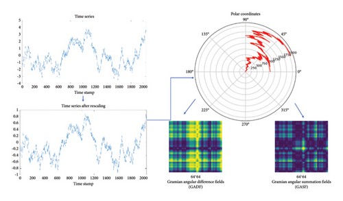
Strong nonlinear data become sparser after GAF processing, eliminating multimodal redundant information, weakening the nonlinearity of the data, and reducing noise [39]. Therefore, using GAF images as model inputs can improve classification accuracy. After encoding time series data into polar coordinates, the use of trigonometric summation and difference helps extract correlation coefficients between time intervals. In this way, GAF can preserve local temporal relationships in a time-correlated form as timestamps increase, which is crucial for pattern recognition [40]. The specific process of GAF is illustrated in Figure 1. After GAF, two kinds of matrixes are obtained under various operation states. Before recognizing them, visualization preprocessing is necessary. GASF and GADF matrixes of a fused signal are transformed into two digital images with a size of 64 × 64.
3. Recognition Method
3.1. DSC
As the fused signal is visualized in the GAF image in Section 2.2, the task of recognizing operational states becomes a task of image recognition. The vibration signal in hydroelectric generating units often contains significant noise caused by internal flow fields and electromagnetic interactions. GAF images from different operational states have complex patterns that are difficult to identify. Considering that CNN is currently one of the most effective methods for image recognition, a model based on CNN has been utilized [41].
In the real-time monitoring of units, computational efficiency is of paramount importance, and the application of traditional CNNs is challenging. In traditional CNNs, each filter performs a full convolution operation across all input channels, resulting in a relatively high computational cost, especially for deep networks or large inputs. Moreover, CNNs typically contain numerous parameters due to the use of full convolutions, which can lead to overfitting, especially when the training data for hydroelectric units is limited.
To address the problems mentioned above, DSC is used to reduce computational complexity. As shown in Figure 2, DSC consists of two sequential convolutional operations: depthwise convolution and pointwise convolution. The depthwise convolution applies a single filter per input channel to capture the spatial correlations, and the pointwise convolution performs 1 × 1 convolutions to combine information across channels. Thus, the depthwise convolution requires fewer parameters and operations than standard convolutions, making it more computationally efficient. Pointwise convolution further reduces dimensionality. With fewer parameters, the efficiency is improved and the risk of overfitting is reduced by the DSCNN models [42].
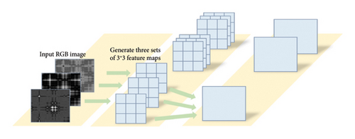

CNN and DSCNN are compared in Figure 2. In CNN, a convolutional kernel with a size of 3 × 3 is used, requiring 81 parameters (3 × 3 × 3 × 3 = 81) for training and adjustment. In contrast, in Figure 2(b), the total number of parameters is the sum of the two steps, requiring only 36 parameters (3 × 3 × 3 + 3 × 3 = 36). This shows that DSC can significantly reduce the number of model parameters and computational workload.
3.2. MobileNetV3
The MobileNet model is a typical DSCNN architecture commonly used in mobile and embedded devices [43]. It enables efficient real-time operations on mobile devices with reduced computational load, making it particularly suitable for the real-time monitoring of hydroelectric generating units. Therefore, an improved version named MobileNetV3 is used in this work. The structure of the established model is described in Table 1.
| Input | Operator | Exp size | Out | SE | NL | s |
|---|---|---|---|---|---|---|
| 2242 × 3 | Conv2d, 3 × 3 | — | 16 | — | HS | 2 |
| 1122 × 16 | Bneck, 3 × 3 | 16 | 16 | √ | RE | 2 |
| 562 × 16 | Bneck, 3 × 3 | 72 | 24 | — | RE | 2 |
| 282 × 24 | Bneck, 3 × 3 | 88 | 24 | — | RE | 1 |
| 282 × 24 | Bneck, 5 × 5 | 96 | 40 | √ | HS | 2 |
| 142 × 40 | Bneck, 5 × 5 | 240 | 40 | √ | HS | 1 |
| 142 × 40 | Bneck, 5 × 5 | 240 | 40 | √ | HS | 1 |
| 142 × 40 | Bneck, 5 × 5 | 120 | 48 | √ | HS | 1 |
| 142 × 48 | Bneck, 5 × 5 | 144 | 48 | √ | HS | 1 |
| 142 × 48 | Bneck, 5 × 5 | 288 | 96 | √ | HS | 2 |
| 72 × 96 | Bneck, 5 × 5 | 576 | 96 | √ | HS | 1 |
| 72 × 96 | Bneck, 5 × 5 | 576 | 96 | √ | HS | 1 |
| 72 × 96 | Conv2d, 1 × 1 | — | 576 | √ | HS | 1 |
| 72 × 576 | Pool, 7 × 7 | — | — | — | — | 1 |
| 12 × 576 | Conv2d 1 × 1, NBN | — | 1024 | — | HS | 1 |
| 12 × 1024 | Conv2d 1 × 1, NBN | — | K | — | — | 1 |
- Note: In Table 1, the first column “Input” in the table indicates the shape changes of each feature layer in the model. A dash “-” signifies that the layer cannot perform the corresponding operation. The “Attention Module” column with “√” indicates that the layer uses the attention module (squeeze and excitation [SE]). In the “Operator” column, “Bneck” represents the block unit of MobileNetV3, “3 × 3” indicates the size of the convolution kernel used in that layer, and “NBN” denotes the absence of batch normalization in the convolution layer. “Exp size” represents the number of convolution kernels of the first layer 1 × 1 Conv2d in each Bneck block. “NL” denotes the nonlinear activation function used in each layer, where “RE” indicates the use of the ReLU activation function, “HS” indicates the h-swish function, and “K” for the model output layer represents the number of types of conditions to be identified. The last column “s” represents the stride used in each block structure.
In the MobileNetV3 model, the classification layer mainly includes global average pooling and multiple point convolution layers in DSC. Since the global average pooling compresses the features to one point, some spatial information is missing and leads to a reduction in the classification accuracy. To solve the problem of information loss, a SE block is introduced in MobileNetV3. The SE module enhances the sensitive features in figures with operations of SE, and the ability of expression for faults in established models can be enhanced without an increasing computational load.
4. Result and Discussion
4.1. PCA–GAF–DSCNN Method
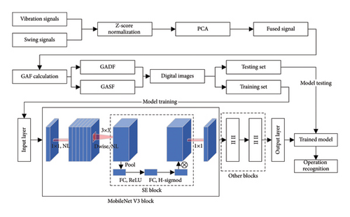
Based on the information provided in Sections 2 and 3, the PCA–GAF–DSCNN method is illustrated in Figure 3. In this approach, multichannel vibration and swing signals are fused using PCA and then transformed into digital images using GAF. Subsequently, DSCNN models are constructed for operation recognition. The PCA–GAF–DSCNN model is developed using Python 3.8 and implemented within a browser/server (B/S) architecture, hosted on the server of the hydroelectric power station data service center.
4.2. Description of Data
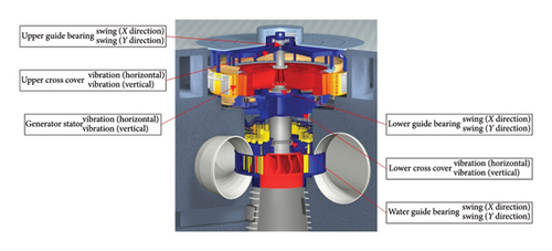
To verify the correctness of the method, we used and analyzed vibration and swing signals collected from a Kaplan turbine at a hydroelectric power station in Southwest China. The hydroelectric unit has a rated power of 175 MW. Monitoring signals were obtained from 12 channels with a sampling frequency of 1024 Hz, including 6 groups of swing signals and 6 groups of vibration signals. The locations for specific testing and data collection are listed in Table 2, and the detailed arrangement of these positions is illustrated in Figure 4.
| No. | Testing and collecting positions |
|---|---|
| 1 | Upper guide bearing, swing (X direction) |
| 2 | Upper guide bearing, swing (Y direction) |
| 3 | Lower guide bearing, swing (X direction) |
| 4 | Lower guide bearing, swing (Y direction) |
| 5 | Water guide bearing, swing (X direction) |
| 6 | Water guide bearing, swing (Y direction) |
| 7 | Upper cross cover, vibration (horizontal) |
| 8 | Upper cross cover, vibration (vertical) |
| 9 | Generator stator, vibration (horizontal) |
| 10 | Generator stator, vibration (vertical) |
| 11 | Lower cross head, vibration (horizontal) |
| 12 | Lower cross head, vibration (vertical) |
Five different operation states of the unit are chosen, including working under rated power, partial load, no-load state, changing speed state, and unstable operation states. Among these, unstable operation states typically occur during extremely low power or when some mechanical faults arise, and this operation state should be avoided in routine operations.
The monitoring signal is recorded as a series of sequences with a length of 2048 data points over two seconds. Each GADF or GASF image is then obtained based on these 2048 data points. The swing signal in the upper guide bearing of the Y direction and the vertical vibration signal of the upper cross cover are selected for comparison with the fused signal. Both GADF and GASF images are calculated and used. Therefore, six groups of samples are chosen here to compare the different original signals and fused signals, as shown in Table 3.
| Group | Signal source | Image |
|---|---|---|
| A | Swing signal of upper guide bearing in Y direction | GADF |
| B | Vertical vibration signal of upper cross cover | GADF |
| C | Fused signal based on PCA | GADF |
| D | Swing signal of upper guide bearing in Y direction | GASF |
| E | Vertical vibration signal of upper cross cover | GASF |
| F | Fused signal based on PCA | GASF |
4.3. Data Fusion and Visualization
All signals in Table 2 are analyzed based on PCA described in Section 2.1. The fused signal from vibration and swing signals under normal operation state is shown in Figure 5(c), and the original vibration and swing signals in Y-direction are shown in Figures 5(a) and 5(b). The fused signal captures the main trend of all signals. By using the fused signal to replace the signals from the 12 channels, the computational cost is significantly reduced.
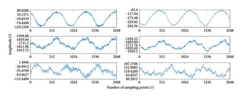
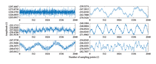

From Table 3, six groups of samples were extracted, each containing states of rated power, partial load, unstable running, no load, and changing speed. Different operation states are named States A to E, respectively. The rated power, which is the optimal running state for the unit by design, is approximately 175 MW in this case. The partial load state occurs when a generating unit must face adjustment missions according to the requirements of other power stations or regional power grids, and it is not recommended to run in this state for a long time. Unstable running also occurs during similar adjustment missions when the output power is significantly lower than the rated power. In the unstable state, vibration and swing increase substantially, which may lead to a high risk of equipment damage, and this state necessitates vigilant monitoring and proactive measures. No load and changing rotation speed occur during the processes of startup, shutdown, and adjustment and are difficult to directly identify based on the original signals.
As depicted in Figures 6 and 7, the GASF and GADF images obtained through GAF for samples under different operation states are extracted from the six groups of samples in Table 3, respectively. The GASF and GADF images obtained from a single signal typically exhibit relatively simple features. This results in limited features in the images, making it difficult to fully showcase the complex behavioral characteristics of the unit under different states. In contrast, the GASF and GADF images obtained from the fused signal have stronger discrimination capabilities and contain more information, which can more accurately reflect the unit states, thereby improving model performance. For detailed information on the impact of model performance, please refer to Section 4.5.


4.4. Modeling and Training
The PCA–GAF method is taken for transforming signals into images as it maintains the coherence between the operation state and running vibration–swing data required for recognition. Corresponding GADF and GASF images obtained are shown in Figures 6 and 7, and a graphical representation of different states of GAF is presented. After this conversion, parameters of the established MobileNetV3 model can be trained and validated according to these images as input. The MobileNetV3 model was established under a Python 3.9 environment based on a TensorFlow framework.
As shown in Table 4, each data group is then divided into a training set, validation set, and test set. The training set is for model learning, and the validation set is for tuning and early performance assessment. The test set is for evaluating the final performance of the model on unseen data. There are 1265 samples used in this work and the ratio of three sets is near to 3:1:1. Each sample has a length of 2048 points and is changed into a 64 × 64 size image. Due to limited data collection for the hydroelectric unit, there is inconsistency in the number of samples across different operation states.
| Sets | Rated power | Partial load | Unstable running | No load | Changing speed | Total number |
|---|---|---|---|---|---|---|
| Training set | 100 | 163 | 241 | 117 | 135 | 756 |
| Validation set | 33 | 54 | 80 | 39 | 45 | 251 |
| Test set | 35 | 55 | 82 | 40 | 46 | 258 |
Six groups of MobileNetV3 models are established according to GADF and GASF images according to Table 3 correspondingly and trained with the training set and validation set. The test set is used to prove the effectiveness of the models, which did not participate in the training process. Group A and Group D are built from the swing signal of the upper guide bearing in the Y direction, while Group B and Group E are from the vertical vibration signal of the upper cross cover, and all these four are used to make a comparison of recognition results between the original signals and the fused one.
4.5. Recognition Result and Discussion
To avoid the potential occurrence of overfitting, an L2 regularization term is added to the loss function during model training. The training parameters have also been adjusted and optimized, with a batch size of 32 and a learning rate is 0.001. The curves of total loss and accuracy rate in Figures 8 and 9 indicate that the model training is still satisfactory, and there is no apparent overfitting phenomenon after regularization.
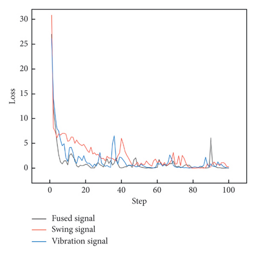
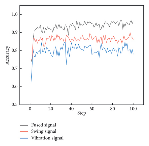
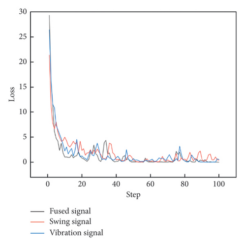
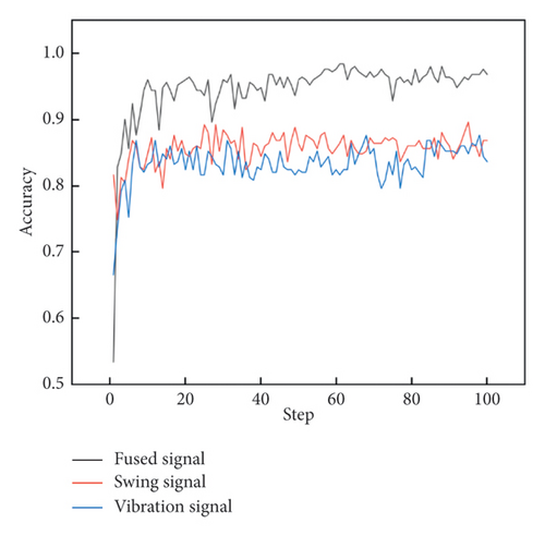
Among the three types of signals, fused signals based on PCA–GAF have the fastest convergence speed and achieve 100% accuracy in the training process, compared to the swing or vibration signals which reach approximately 99%. The results of the operation state recognition for the hydroelectric unit are recorded in Table 5, showing that PCA–GADF and PCA–GASF achieve accuracies of 95.21% and 96.41% in the test set, respectively.
| Signal source | Accuracy in training set (%) | Accuracy in testing set (%) |
|---|---|---|
| Group A | 99.47 | 87.65 |
| Group B | 99.87 | 79.68 |
| Group C | 100.00 | 95.21 |
| Group D | 99.47 | 84.86 |
| Group E | 99.60 | 86.45 |
| Group F | 100.00 | 96.41 |
Confusion matrices for all models are calculated to specifically evaluate their performance. The recognition results from Group A to Group F, based on GADF and GASF, are shown in Figures 10(a), 10(b), 10(c), 10(d), 10(e), and 10(f) respectively. As demonstrated in these figures, models established with integrated signals perform better than others, with both Group C and Group F achieving an accuracy of over 95% in the test set.
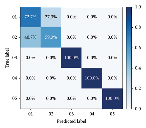
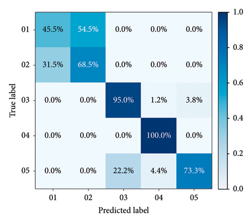
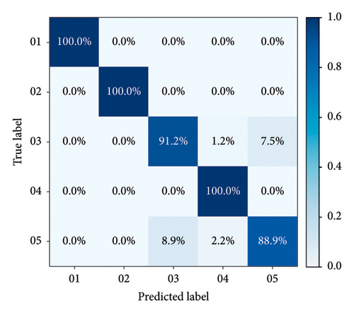
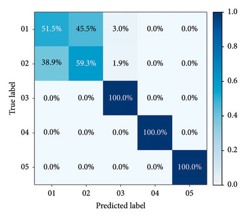
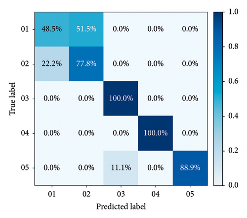

In the confusion matrices of Groups A, B, D, and E, distinguishing between rated power and partial load operations proves to be more challenging, whereas other operational states are easier to identify. This difficulty arises because rated power and partial load operations are similar, as both states involve the units being relatively stable, with the primary differences being in output electricity and unit load. Consequently, the single vibration and swing signals in the upper area of the hydroelectric generating unit are not distinctly noticeable. However, when the vibration and runout signals from various parts of the unit are fused, as seen in Groups C and F, these two operation states can be successfully differentiated. During unstable running and changing speed states, the vibration and swing signals exhibit complex patterns, leading to a certain level of mutual misjudgment between these states. In contrast, during the no-load state, the flow-through components are almost unaffected by the water flow, resulting in simpler mechanical characteristics and thus higher recognition rates. Overall, the proposed model in Figures 10(c) and 10(e) effectively addresses recognition difficulties, achieving an accuracy of over 95%, and performs better than models based on single-channel signals.
PCA reduces the dimensionality of high-dimensional data by projecting it onto a new set of orthogonal axes through linear transformation and ranks the principal components according to their variance, thus achieving redundancy reduction and data compression. In the experiment, multichannel signals were merged into a single signal, which inevitably led to information loss due to the inherent limitations of signal fusion methods. This was also a contributing factor to the slight decrease in accuracy when detecting unstable operations and changes in speed. However, as shown in Tables 5 and 6, data fusion significantly enhances overall recognition accuracy, with its benefits far outweighing its drawbacks.
| Signal source | One epoch (s) | Signal source | One epoch (s) |
|---|---|---|---|
| Group A | 17.24 | Group D | 16.96 |
| Group B | 17.19 | Group E | 17.12 |
| Group C | 16.62 | Group F | 16.63 |
4.6. Evaluation for Time Consumption
4.6.1. Training Time
A computation time for model training with the PCA–GAF method is calculated. GAF images from the original vibration and swing signals are used for the comparison. A personal computer with Windows 10.0 system is utilized for calculation, with a CPU of Core i5-12400F and a RAM of 16 GB. All programs are based on Python 3.9.
The result is recorded in Table 6 and PCA–GAF images consistently have a shorter training time. This is because PCA compresses data while also retaining most of the information in the data. Therefore, when training deep learning models using GADF and GASF from fused signals, the model often converges faster, thus accelerating the training speed.
4.6.2. Inference Time
To evaluate the real-time implementation effectiveness of the proposed method, an analysis for inference time is necessary. The total inference time is mainly comprised of image generation time and model recognition time. To ensure the recognition model runs normally, the inference time has to be less than the acquisition time of one signal sequence which is 2 s as shown in Figure 11.
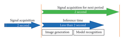
The specific time in each stage for one image is recorded in Table 7. Due to the slight differences in computation time for each sample, we perform the analysis and comparison using the average value. From Table 7, the average value of the inference time is about 0.0289 s which is less than 2s significantly. Thus, the proposed method demonstrates feasibility for practical application.
| Signal source | Image generation time (s) | Model recognition time (s) | Inference time (s) |
|---|---|---|---|
| Group A | 0.0003 | 0.0272 | 0.0275 |
| Group B | 0.0003 | 0.0271 | 0.0274 |
| Group C | 0.0004 | 0.0282 | 0.0286 |
| Group D | 0.0005 | 0.0293 | 0.0298 |
| Group E | 0.0003 | 0.0285 | 0.0288 |
| Group F | 0.0006 | 0.0304 | 0.0310 |
4.7. Comparison Analysis
In this study, the operation recognition challenge of hydroelectric generating units is transformed into an image recognition task. Considering the high dependency of deep learning models on data, it is essential to compare CNN with other image recognition methods based on conventional features to assess the effectiveness of the proposed method. In Section 4.6, a series of models based on conventional features are introduced, including local binary patterns (LBPs), Tamura texture features (Tamura), and second-order gradient (SOG). SVM is employed as the classification tool for these features. These methods were chosen due to their widespread use and proven effectiveness in image recognition applications.
To prevent overfitting during model training, image augmentation is performed, including flipping, scaling, random rotation, vertical scaling, and adding noise to the samples before training. The transformations do not alter the essential information within the images. Their primary purpose is to enhance the model’s robustness to variations in scale and orientation. These transformations preserve the spatial relationships and pixelwise patterns in the images, ensuring that the physical meaning of the data remains largely intact. In other words, the augmented images continue to retain the meaningful signals needed for interpretation, as the original geometric structure is preserved and meaningful data can still be decoded from these transformations [44, 45]. Meanwhile, a 5-fold cross-validation is also applied in the training process. Through multiple splits and validations, the random errors caused by a single data split were effectively reduced, which improved the generalization performance of models.
The comparison results shown in Figures 12(a) and 12(b) highlight the accuracy rates based on LBP and SOG features, reaching 75.89% and 92.22%, respectively, in the training set. However, Tamura features exhibit a significantly lower accuracy rate of approximately 30%. Notably, there is a discernible decrease in accuracy rates across all feature groups in the testing set. Among the various image texture features examined, SOG demonstrates the highest training accuracy, closely approaching that of the proposed method. However, its testing accuracy values experience a notable decline. Regarding the recognition problem for PCA–GAF images derived from hydroelectric generating units, the performance of traditional features appears notably inferior to that of deep learning methods, with the proposed method achieving the most favorable outcome.
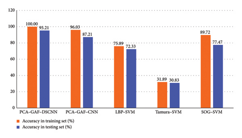
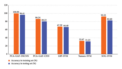
Furthermore, DSCNN models exhibit superior performance compared to a typical CNN model. The CNN model employed here consists of a feature extraction component and a classification component. The feature extraction part comprises three convolutional layers, each followed by a ReLU activation function and a max-pooling layer. The classification part includes two dropout layers, two fully connected layers, and one ReLU activation function. DSCNN achieves testing accuracy rates of 95.21% and 96.41%, outperforming CNN rates of 87.21% and 80.23%, respectively, thus indicating the positive impact of DSC in this context.
5. Conclusion
This paper proposes a novel recognition approach for operation states of hydroelectric generating units based on data fusion and visualization techniques. According to the running data from a Kaplan hydroelectric unit in a hydropower station located in the southwest of China, the proposed PCA–GAF–CNN method has been proven to be effective and accurate. The proposed method enables the identification of abnormal states, making it applicable for use in monitoring and fault diagnosis.
First of all, considering that operation states of hydroelectric generating units can be reflected through vibration and swing signals, PCA is used to remove information redundancy and improve computational efficiency by combining obtained multichannel signals into a fused signal. Second, GAF is used to present features of the fused signals under different operation states in image format as GADF and GASF. Third, a typical DSCNN framework is developed to achieve operation recognition based on image data. The experimental results show that the GADF and GASF of the fused one reach a high accuracy of 95.21% and 96.41% in the respective test sets, compared to 87.65% and 84.86% according to the swing signal of the upper guide bearing in the Y direction, and 79.68% and 86.45% according to the vertical vibration signal of the upper cross cover. Compared to single-channel signals from vibration and swing, the average recognition accuracy is effectively improved. Meanwhile, a comparative analysis is conducted in our research using traditional hand-crafted approaches, and the proposed model reaches the highest accuracy among the five methods.
In subsequent research, we plan to collect more challenging data related to the failure and faults of the hydroelectric units and continuously enhance the performance of the model in limited and small sample learning scenarios.
Conflicts of Interest
The authors declare no conflicts of interest.
Funding
This research was funded by the National Natural Science Foundation of China (Grant nos. 52479087 and 51839010), the Yellow River Joint Fund of the National Natural Science Foundation of China (Grant no. U2443226), and the Shaanxi Provincial Department of Education Collaborative Innovation Center Project (Grant no. 22JY047).
Open Research
Data Availability Statement
The data presented in this study are available upon request from the corresponding author, but the final approval requires the consent of the hydropower station where the equipment is located.


