Due to the intricate chaotic environments encountered in distributed sensor applications, such as sea monitoring, machinery fault diagnosis, and EEG weak signal detection, neural networks often face insufficient data to effectively carry out detection tasks. In contrast to traditional machine learning models, a statistical approach employing multidimensional nonlinear correlation (MNC) exhibits an unparalleled signal pattern prediction capability and possesses a streamlined yet robust framework for signal processing. However, the direct application of MNC to weak pulse signal detection remains constrained. To surmount these challenges and achieve high-precision signal detection, we explore a novel MNC approach, integrating phase reconstruction and manifold broad learning, specifically tailored for distributed sensor fusion detection amidst chaotic noise. Initially, the distributed observational data undergoes phase space reconstruction, transforming it into fixed-size arrays. These reconstructed tuples are then processed through the high-dimensional sequence of manifold broad learning, serving as inputs for the nonlinear correlation module to extract spatiotemporal features. Subsequently, a MNC system augmented with a QRS detector layer is devised to predict and classify the presence of a weak pulse signal. This integrated MNC approach, combining phase reconstruction and broad learning, operates within an enhanced feature space of the source domain, realizing detection fusion across distributed sensors through a majority voting principle. Simulation studies and experiments conducted on sea clutter datasets demonstrate the efficacy and robustness of the proposed MNC method, leveraging phase reconstruction and manifold broad learning strategies, for distributed sensor weak pulse signal fusion detection within chaotic backgrounds.

1. Introduction

1.1. Distributed Structure Universal Detection Fusion System Detection Structure and Current Status

Weak signal detection is a fundamental task in complex and highly chaotic noise environments. Detecting weak signals and extracting useful information in the context of noise is a very difficult task. With the development of modern technology, the first generation systems based on independent sensors are no longer able to solve many problems in reality. Distributed multisensor networks, such as system persistence, low observability, target classification, and recognition, can not only provide a large amount of data but also further obtain the classification characteristics of targets. It is necessary to use this detection model. However, under these noise interferences, especially strong color noise such as chaotic noise or pink noise, it may seriously affect the overall reliability and stability of extracting weak useful signals in distributed sensors. Therefore, it has become very important to develop effective weak signal detection techniques for distributed sensor detection fusion. This research not only represents the development of single sensor signal processing but also contributes to solving the problem of national classification detection fusion.

The centralized distributed sensor fusion detection system is shown in Figure 1, which consists of sensors and a fusion center. u₀(t) = 1 representing the judgment result of the fusion center at time t is that the signal exists; on the contrary, u₀(t) = 0 representing the judgment result of the fusion center at time t is that the signal does not exist.

Details are in the caption following the image — **Figure 1**
Open in figure viewer PowerPoint

General detection fusion system with a distributed structure.

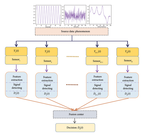
In the distributed multisensor processing system, each sensor first preprocesses the obtained observation data, then transmits the compressed data to other sensors, and finally summarizes it to the fusion center. The data fusion of multiple sensors can generate more accurate, complete, and reliable data than a single sensor. Data fusion can model some uncertainties and fuse various types of information to obtain a more reliable and accurate result. At present, distributed sensor information fusion has received close attention from scholars at home and abroad, and the multisensor collaborative detection technology has been widely used in remote sensing measurement and control, aerospace, intelligent transportation, reconnaissance and detection, and other fields [1–5]. The current information fusion methods mainly include weighted average, Bayesian estimation, Kalman filter, fuzzy logic reasoning, recursive weighted least squares algorithm, and artificial neural network [6–8].

To eliminate the measurement information in the fusion center update equation, a centralized fusion method is proposed, that is, the measurement data are fused by matrix transformation of the global optimal centralized fusion method [9]. The maximum weight multimodal information fusion is trained through a convolutional neural network and outputs decision information, and then, the decision information is fused [10]. Given the lack of an effective information fusion model for heterogeneous multisensors, an improved Dempster/Shafer evidence theory algorithm is proposed to fuse heterogeneous multisensor information. The algorithm solves the problem of the DS evidence theory in dealing with highly conflicting evidence to a certain extent [11].

A weak signal mainly refers to signals with low signal strength, which are small and weak, difficult to be sensed or received by devices, or in the context of strong noise, and the concept of weak is relative to noise [12, 13]. Regarding the detection of weak signals, it is mainly divided into the following types of methods: time-domain analysis/frequency-domain analysis and time-frequency domain analysis. In recent years, enormous different kinds of models, such as traditional statistical methods [14], neural network [15–19], Kalman filter [20–25], and (generalized) likelihood ratio (GLRT) [26, 27], have been successfully applied to fusion detection in distributed sensor networks. Notably, Su et al. [28] combined a local polynomial nonparametric statistical method with Bayesian risk for fusion detection under a chaotic background and constructed a distributed sensor local linear autoregressive (DS-LLAR) model for obtaining the one-step prediction error of each sensor and the corresponding conditional probability density function under each sensor’s hypothesis test.

1.2. Introduction to Generalized Learning, Broad Learning (BL), Phase Space Reconstruction (PSR), and Model Structure

The above-mentioned models have obtained comparatively satisfactory results for fusion detection in distributed networks. However, despite improvements or updates in statistics and machine learning, such approaches involve certain limitations, especially in feature extracting of intrinsic dynamical evolution. A promising method to extract the intrinsic essential characteristics is BL, which enhances feature mining capability in a transformed high-dimensional space. Based on this enhanced features, multidimensional nonlinear correlation (MNC) can be trained using manifold learning. Thus, incorporating BL can help avoid insufficient training. In this study, inspired by the powerful statistical fitting of MNC, we combine the PSR, robust BL, and the MNC to design a statistical learning network architecture for weak signal detection submerged in chaotic noise by fully considering the potential chaotic characteristics of the observed data. To improve the accuracy and reliability of signal detection, we establish an innovative distributed MNC network and apply BL and PR strategy to increase the model prediction efficiency.

Regarding MNC, Kachouie and Deebani [31] proposed that the correlation factor (AF) performs much better than distance discrimination and Pearson correlation in identifying linear and nonlinear relationships under noisy conditions. Zhu et al. proposed a method for nonlinear extension of FCCA, which uses distance covariance and distance correlation to reveal the correlation between variables and recommended FSCA-DC as the most stable and useful method. The distributed MNC network used in this paper is used to study multidimensional nonlinear data. The following is a detailed introduction to the model:

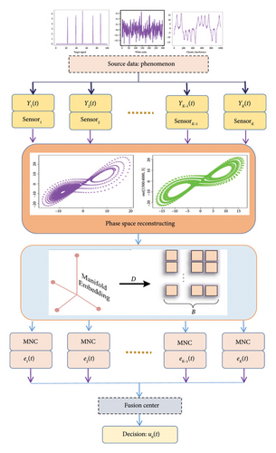
This article’s model processes observation signals into multidimensional fixed size array signals through PSR and manifold generalized learning. Then, in a distributed fusion system, based on extracting sequence correlations, an MNC model with distributed sensor PR and BL systems is established to obtain prediction errors. Then, a threshold for the QRS detector is constructed to detect the signal by performing differential processing on the error sequence. Finally, a final decision is made after fusing the detection results of each sensor. The proposed method can obtain potential representational features through manifold learning and PR in the source domain.

1.3. Contribution and Structure of This Article

The main innovative contribution of our work can be summarized as follows:

1.
A novel MNC model is developed via PSR and BL. This study develops a statistical nonlinear correlation architecture for distributed sensor weak signal fusion detection, with the most suitable improvements to process 1-D signals with chaotic interference. In contrast to traditional machine learning networks, the MNC that relies entirely on the nonlinear correlation exhibits a superior inherent extracting capability of nonlinearity, interpretability, and low computing complexity.
2.
The 1-D observed signal is interpreted as a sequence of fixed-sized tuples for characterizing attractors and intrinsic evolution. We creatively mix up the phase space delay embedding and manifold BL embedding with more detailed information on the array sequence, which is appropriate for the MNC architecture. Additionally, an MNC model with a fusion classifier is incorporated in the hybrid detecting model to process the output predicted residuals of the MNC with the useful targeting signal and perform high precision classification.
3.
The investigated approach can detect weak signals while using a limited number of observed samples associated with different scenarios. By incorporating the BL techniques and QRS detector, the MNC with simple parameter estimation can be efficiently fitted in the multidimensional phase space and be promptly completed for the fusion detection tasks without pretraining or fine-tuning.
4.
Combining models with BL can help avoid insufficient training; BL and PR strategies to improve model prediction efficiency; established MNC models for distributed sensor PR and BL systems to obtain prediction errors; detecting signals by performing differential processing on erroneous sequences. After integrating the detection results of each sensor, make the final decision. The method studied can detect weak signals while using a limited number of observation samples related to different scenarios. By combining the BL technology and the QRS detector, MNCs with simple parameter estimation can effectively fit into multidimensional phase space and quickly complete fusion detection tasks without pretraining or fine-tuning. In summary, the role of each element is absolute and will to some extent affect the detection accuracy of the entire detection model.

The MNC architecture proposed in this article combines PR and BL techniques. The MNC model adopts multiparty robust extensive learning in the reconstructed phase space, without relying on extensive and complex training samples to demonstrate its outstanding feature extraction and pattern classification capabilities. Compared with traditional two-dimensional and multidimensional information fusion methods, it has significant advantages in terms of computational cost and dependence on samples.

The structure of following parts of this article is organized as follows: the second part introduces the distributed signal detection problem under chaotic interference; the third part proposes the distributed detecting fusion system; the fourth part is the simulation and real data experiment; and the last part is the conclusion.

2. Distributed Signal Detection Problem Under Chaotic Interference

In distributed signal detection, the challenges brought by chaotic interference mainly include three points: distinguishing between signals and interference, multinode collaboration, and data fusion. Under chaotic interference, it becomes more difficult to distinguish between real pulse signals and noise. Due to the randomness and unpredictability of chaotic interference, multiple nodes need to effectively collaborate to jointly detect signals. How to effectively fuse data from different nodes to reduce the impact of chaotic interference is a key issue. Pulse signals have temporal discreteness and amplitude variability, and pulse shape deformation, pulse arrival time jitters, and pulse missing or repeating are all very easy to occur. Model detection implements detection algorithms at various nodes and collects detection results to effectively reduce errors and make detection results more accurate.

The problem of detecting weak pulse signals in chaotic noise can be abstracted into the following hypothesis testing problem:

()

where y_i(t) is the observation signal of the ith sensor,

is the chaotic noise background signal of the ith sensor, s(t) represents the weak impulse signal and is independent of the chaotic noise

, n_i(t) represents the white noise with a mean of 0, and c_i(t) represents the sum of chaotic noise background signal

and white noise n_i(t).

Because the weak pulse signal s(t) is submerged in the chaotic noise background signal

, if the hypothesis in formula (1) is used for hypothesis testing, it cannot detect whether the observed signal y(t) contains s(t). Therefore, the interference of the chaotic noise signal

should be removed first. At this time, the hypothesis of formula (1) is transformed into the hypothesis testing problem of formula (2):

()

In the distributed fusion detection system, the judgment result made by each sensor and the fusion center is a binary classification problem, which means that the signal exists. Therefore, the hypothesis test of formula (2) is transformed into

()

When is true, the judgment results of the sensor and the fusion center are both 0, which means that the signal does not exist. When is true, the judgment results of the sensor and the fusion center are both 1.

3. Proposed Distributed Detecting Fusion System

Nonlinear correlation, which employs the multidimensional stacking structure, possesses strong dependency extraction ability and low computational complexity. In this study, we creatively apply the nonlinear correlation architecture to develop a novel hybrid model for weak pulse signal detection in a chaotic background, namely, MNC. To make this model fully suitable for processing 1-D-received time series signals, some reasonable improvements are made. Additionally, since it is relatively coarse to direct application for predicting of inadequate quality samples, it is better that the PSR and the BL technique are utilized to enhance the feature capturing capability of the MNC model for weak signal detection tasks. The proposed MNC model with PR and BL strategies is established and applied for weak pulse signal fusion detecting, as depicted in this section.

3.1. MNC Architecture

An overview of the MNC architecture for distributed detecting fusion of weak pulse signals under the background of chaotic noise is shown in Figure 2. represents the raw observations of the ith sensor. Specifically, y is reconstructed into b-D tuples , where τ represents the delay time and b represents the embedding dimension. e_i(t)(i = 1, 2, …, K) represents the prediction error of each sensor after prediction by MNC, u_i(t)(i = 1, 2, …, K) represents the decision result of each sensor, and u₀(t) is output through the fusion center. Z is enhanced for m-D arrays , where m represents the number of the manifold embedding dimension. Additionally, h represents the length of the effective input tuples for MNC.

Unlike the traditional chaotic time series processing in the task of predicting using auto regression models, we adopt a hybrid process with PR and BL strategies to generate the tuple manifold embedding, which can be expressed as follows:

()

where Θ_τm represents the phase space embedding reconstruction. Since the obtained phase embedding tuples come from the univariate time series signal with intrinsic attractors, it is essential to extract the detailed evolution in the sequence aiming to maintain the nonlinearity. In this article, we mix up the BL technique which is a fast feature enhancer and can amend the deficiency without spatiotemporal information of traditional statistical methods. Note that the BL manifold embedding is formulated through the following:

()

where W_ui(W_ei) and β_ui(β_ei) are randomly generated weights and offsets, and ϕ(·)(ψ(·)) represents the activation function of the mapped feature. The augmented output [A|D] of the feature layer and enhancement layer is used as the input of the output layer.

Assuming that there are m observation signals in total, the multidimensional observation matrix is as follows:

()

where b_j(j = 1, 2, …, m) is the output one-dimensional feature information after BL extraction in the reconstructed phase space. Polynomial functions can be used to approximate nonlinear correlation functions in most cases, so here we use the nonlinear polynomial functions to approximate their correlations, and the nonlinear effects between multiple variables can be expressed in a polynomial form. The multiple observation state space is defined as (b₁, …, b_m), and the Hadamard product is used to represent the coupled nonlinear relationship between the component b_i and the component b_j, which is b_ij. We suppose that the second-order nonlinear term of the correlation function is N₂ = {b_ib_j|i, j = 1, 2, …, m}, and then, the third-order nonlinear term is N₃ = {b_ib_jb_k|i, j, k = 1, 2, …, m}. By analogy, it can be applied to higher-order nonlinear terms, and these kinds of nonlinear terms can be added to the correlation function by refining the state space as b = {b_i, b_ib_j, b_ib_jb_k, …}(i, j, k = 1, 2, …, m).

Considering the dynamic evolution of variables, the correlation of the derivative signal with the original signal plays an important role. If we choose the variable b_i to predict, the nonlinear correlation characteristic between the derivative signal

and the original signal b_k is

. Thus, the second-order nonlinear term with

can be defined as follows:

()

Additionally, we consider higher-order nonlinear terms with

. For the convenience of describing the prediction process, only the second-order nonlinear term is used here. The phase space is redefined as follows:

()

Next, the PSR of the kth observed variable y_k is as follows:

()

Here, τ is the delay time parameter, and y and Y_k are both dimensional phase spaces.

()

where P is a parameter matrix composed of coupling relationship coefficients. P_i,j and y_k(N + k) are unknown, and b and Y_k are known from row 1 to row N − (m − 1)τ, so define the first row of y and Y_k to N − (m − 1)τ row as

and

()

Then, by solving an equation

, we get

. Then, we can obtain the predicted value as follows:

()

For the weak signal detecting of the single sensor in the output of MNC, we apply the QRS detector [21] to the predicted residuals of MNC, which is a self-learning algorithm for determining the threshold. For distributed sensors, K sensors work at the same time and receive signals at the same time. Therefore, there will be no time difference problem, which also overcomes the defects of the self-learning algorithm due to time difference and has the advantage that the self-learning algorithm can solve individual differences. To eliminate the excessively large difference value caused by the occasional spike and remove the maximum and minimum values of the error difference sequence, it is possible to avoid the missed detection caused by the excessively large threshold to a certain extent; meanwhile, some small difference values can also be removed. To avoid false detection caused by a too small threshold, this can reduce the probability of missed detection and false detection. After removing the maximum value and the minimum value of the error difference sequence, the arithmetic mean of the remaining difference values is calculated, and the detection threshold of the ith sensor is directly obtained as follows:

()

where q is the length of the difference sequence. If Δe_i(t) ≥ h_i, it is considered that there exists a weak pulse signal in the ith sensor at time t; otherwise, it is considered that there does not exist a weak pulse signal. In this study, for distributed multisensor observations, the majority principle is used to judge whether there exists a weak pulse signal in the source signal under chaotic interference. At a certain moment, when two or more of the three sensors detected that there exists a weak pulse signal, the fusion center decides that there exists a weak pulse signal. Conversely, if there is only one sensor in the three sensors or no sensor detected, it shows that there does not exist a weak pulse signal, and the final decision is made by the fusion center.

3.2. Algorithm Procedure of the Presented Approach

In this article, we introduce an innovative MNC architecture that integrates PR and BL techniques for intelligent fusion detection of weak pulse signals using distributed sensors within a chaotic background. Unlike conventional machine learning networks, the MNC model, which employs manifold robust BL in the reconstructed phase space, does not rely on extensive and complex training samples to demonstrate its outstanding feature extraction and pattern classification capabilities. Instead, the BL-based mixed PSR approach is leveraged to enhance the chaotic evolution and intrinsic feature multidimensional manifold embedding abilities of the nonlinear correlation model. In the PSR phase, the received source data are transformed into a higher dimension using time delay and embedding dimension, paving the way for subsequent feature learning. During the feature enhancement stage, the BL system, with its sole feature mapping component, is augmented to swiftly adapt to fit future observations with minimal samples and low computational overhead. The general methodology for distributed weak signal fusion detection is outlined as follows:

Step 1: Acquiring raw observed signal data from all distributed sensor networks and labeled target data in different time domains.
Step 2: Reconstructing 1-D signals as arrays in phase space, respectively, for every distributed sensor.
Step 3: MNC model is developed with nonlinear correlation and manifold robust BL and QRS detector.
Step 4: Training the MNC model adequately using labeled data and testing it using unlabeled data.
Step 5: Obtaining the final fusion result with the QRS threshold discriminant method and fusion rules.
Step 6: Verifying the effectiveness and robustness of the presented model by using different scenarios. Detailed algorithm flow is shown in pseudo code Algorithms 1 and 2:

Algorithm 1: Training and testing MNC model.

Input: y
Output: equation (12)
1.
Initialization;
2.
Divide y into labeled data y_i and unlabeled data y_j;
3.
Training model using labeled data y_i
4.
For i ← 1 to m do{
5.
z_i ← y_i using equation (4);
6.
b_i ← z_i using equation (5);
7.
} end
8.
B ← (b₁⟶b_m) using equation (6);
9.
Predicted variable b_i, taking two-dimensional nonlinear term with as an example;
10.
Redefine phase space b ← using equation (8);
11.
Y_k ← using equation (9)//τ indicates the delay time parameter;
12.
Y_k ← using equation (10)//P is a parameter matrix composed of coupling relationship coefficients
13.
← using equation (11)//define the first row of and to row as and ;
14.
Equation (12) ← ;
15.
For j ← 1 to n do {
16.
Testing model using unlabeled data y_j;
17.
} end
18.
Obtain MNC model;

Algorithm 2: Integration mechanism.

Input: equation (12)
Output: u_i(0)
QRS prediction residual:
1.
Initialization;
2.
value = 0;
3.
h_i and △e_i(t) ← using equation (13);
4.
For i ← 1 to 3 do//Three sensors, each scored {
5.
if
6.
value = value + 1//One point;
7.
u_i(0) = 1//exist; //Judgment result of one of the three sensors
8.
} end
9.
} end
10.
value ⟶ Fusion center:
11.
if value ≥ 2 {
12.
u_i(0) = 1;//exist
13.
else {
14.
u_i(0) = 0;//nonexistents
15.
} end

4. Experimental Results and Analysis

To comprehensively verify the capability, effectiveness, and robustness of the proposed MNC distributed sensor detection fusion, the following simulation experiments are carried out in this section. In the experiments, it is assumed that the three sensors are independent of each other and have the same performance. All three sensors use the Lorenz system to generate chaotic noise background signals. All the white noise sequences obey a normal distribution with a mean of 0 and a variance of 0.01. Experiments were carried out using the observed signals with different signal-to-noise ratios. Simultaneously, some related comparisons with existing methods and detailed analysis are investigated in different scenarios.

4.1. Scenario 1: Simulated Experiments

To test the performance of the presented detecting method under chaotic interference, we simulate the chaotic noise using the Lorenz system, regarding the first component as chaotic noise with the fourth-order Runge–Kutta solving technique. The Lorenz system is as follows:

()

According to the reconstruction, BL strategy, and weak pulse signal detecting, four kinds of simulated experiments are designed in this section. To verify the efficacy of MNC, the samples of the observation signals are different, and it is decided by the designed situation. The main symbols of the four experiments are listed in Table 1. The points at different times are selected as the chaotic background signals of the three sensors, respectively. Additionally, to guarantee the consistency of different experiments, all codes are run on the same hardware and software environment, including Intel CPU and Python.

Table 1. Main symbols.

Symbol	Meaning
y_i(t)	Observed signal
	Chaotic noise
s(t)	Weak pulse signal
n_i(t)	White noise
c_i(t)	Sum of chaotic and white noise
σ	10
r	28
a₂	7
u_i(t)	Decision result
e_i(t)	Prediction residual
τ	Delay time
m	Embedding dimension
h_i	Detection threshold
λ	8/3
a₁	6.5
σ²	Variance

Due to the complexity of the practical environment, the target signal is usually submerged in a chaotic background and various distributed unrelated sensors. We also use SNR to evaluate the performance of the proposed method for pulse signal detecting under strong chaotic noise; here, the SNR can be defined as .

Experiment 1. Weak pulse signal detection experiment, assuming that the pulse signal is a single pulse signal s(t) = a₁s₁(t):

()

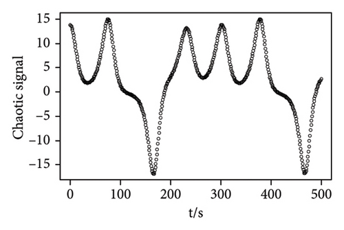
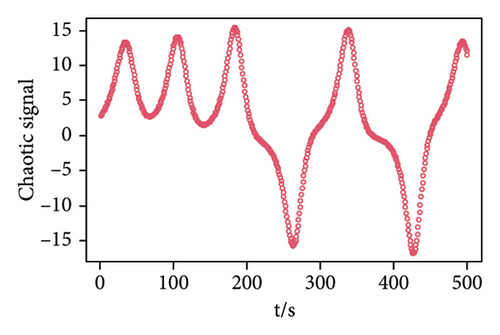
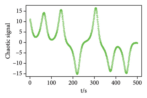
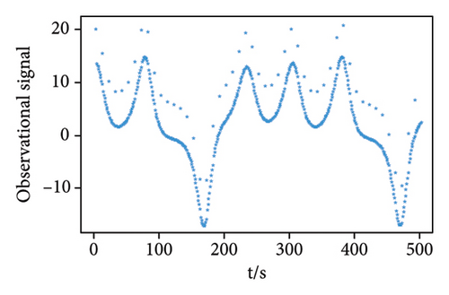
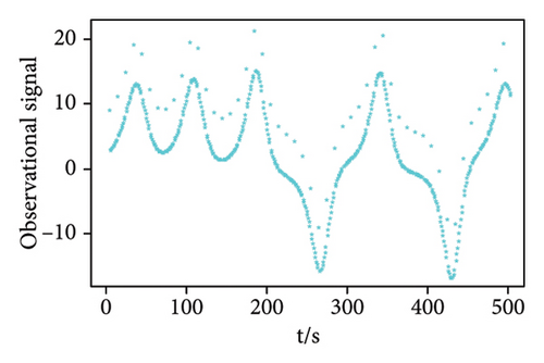
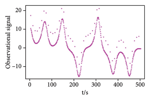
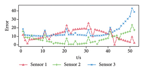
We generate a time series of length 500 as the weak pulse signal, and the signal-to-noise ratio is SNR = −69.8099 dB. Then, the white noise sequence and the weak pulse signal are superimposed on the chaotic background signal, and then, the chaotic noise background signal and the observation signal are shown in Figure 3. Based on the received signals submerged in chaotic interference, the MNC function prediction method is used to fit the signal to obtain the prediction error. The prediction error is forward-differentiated, and the detection threshold is obtained by the proposed approach. Finally, detection and fusion are used to determine whether there is a weak pulse signal. Table 2 shows the simulation parameters when SNR = −69.8099 dB.

Table 2. Simulation parameters when SNR = −69.8099 dB.

Observation signal	Embedding dimension	Delay time
y₁(t)	9	9
y₂(t)	7	9
y₃(t)	7	9

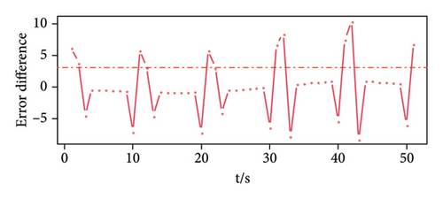
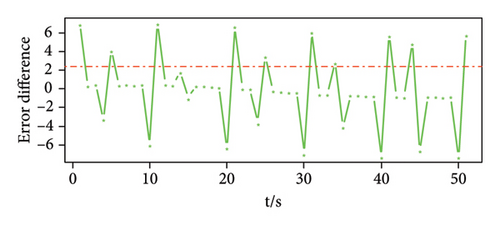
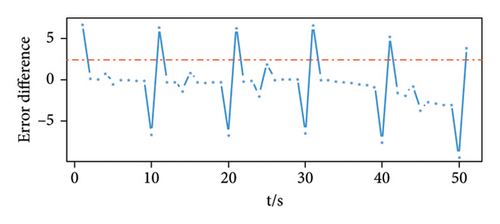
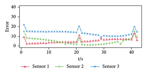
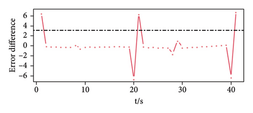
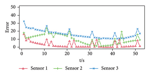
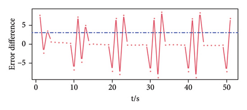
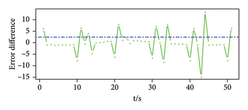
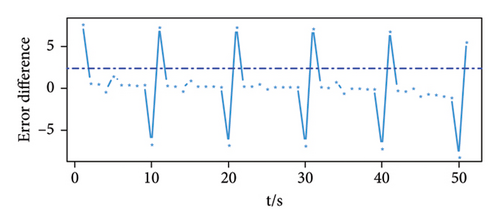
Figure 4(a) shows the prediction error of the three-dimensional signal. It can be seen that the three sensor error values have obvious peaks at the time when the signal is set, such as at times 0, 10, 20, 30, 40, and 50. In addition, the prediction errors obtained by the three sensors have a similar law, that is, the error value at the moment when the signal appears is maximum in an interval. Figures 4(b), 4(c), and 4(d) are the prediction error difference sequence diagrams of the three-dimensional signal, and the red dotted line in the figure is the threshold value obtained by calculation. The time corresponding to the threshold value and the error difference value above the threshold value is the time when a weak pulse signal is detected. On the contrary, it is considered that there is no weak pulse signal at this moment.

Experiment 2. Weak pulse signal detection experiment, assuming that the pulse signal is a single pulse signal, s(t) = a₁s₁₁(t), t = 20, 40, 60, ….

We generate a time series of length 500 as the weak pulse signal, and the signal-to-noise ratio is SNR = −73.0940 dB. Table 3 shows the simulation parameters when SNR = −73.0940 dB.

Table 3. Simulation parameters when SNR = −73.0940 dB.

Observation signal	Embedding dimension	Delay time
y₁(t)	9	6
y₂(t)	6	11
y₃(t)	5	12

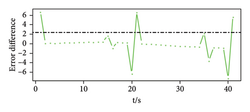
The conducted process is similar to the situation in Hypothesis (1), and the regularity of the peaks of the prediction errors of the three sensors can be seen in Figure 5 according to the results of the proposed method. The black dotted line in the figure is the detection threshold of the sensor, and the threshold has a good ability to detect whether there is a weak pulse signal.

Experiment 3. Weak pulse signal detection experiment, assuming that the pulse signal is a single pulse signal, s(t) = a₃s₃(t), t = 10, 20, 30, ….

We generate a time series of length 500 as the weak pulse signal, and the signal-to-noise ratio is SNR = −77.8375 dB. Table 4 shows the simulation parameters of the operation in assumption when SNR = −77.8375 dB.

Table 4. Simulation parameters when SNR = −77.8375 dB.

Observation signal	Embedding dimension	Delay time
y₁(t)	9	9
y₂(t)	8	9
y₃(t)	7	9

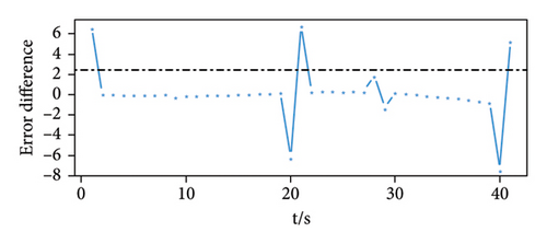
Just as in the case of Hypothesis (1), we can observe the chaotic background and the received signal. By applying the proposed MNC model, we can discern a distinct pattern in the peaks of the prediction errors for the three sensors, as shown in Figure 6. The blue dotted line represents the detection threshold for each sensor, and this threshold effectively detects the presence of weak pulse signals.

Experiment 4. Performance comparison of different models.

The accuracy rate refers to the proportion of objects that are predicted to belong to that category in a certain category. Recall refers to the proportion of all correctly identified objects to all objects that need to be identified. The F1 score is a composite measure of precision and recall, which penalizes extreme cases.

()

where TP is the number of samples with a detected signal, FP is the number of samples with a signal but not detected, FN is the number of samples with no signal but detected as a signal, and TN is the number of samples with no signal detected as no signal number.

Tables 5, 6, and 7 are the detection effects of different models under different signal-to-noise ratios, respectively. Tables 5, 6, and 7 correspond to Figures 7, 8, and 9, respectively, showing the detection effects of different models under different signal-to-noise ratios, where MNC is the multidimensional nonlinear correlation polynomial prediction method in this study, RF is the random forest detecting method, GDBT is the gradient boosting decision tree method of detection, CNN is a convolutional neural network, and LSTM is a long short-term memory network.

Table 5. Detection effects (SNR = −69.8099 dB).

	Accuracy	Precision	Recall	F1 score
MNC	0.9808	0.8571	1.0000	0.9890
RF	0.923	1.0000	0.5000	0.6667
GDBT	0.9615	0.7500	1.0000	0.8571
CNN	0.9585	1	0.6250	0.7692
LSTM	0.9387	1	0.6875	0.8148

Table 6. Detection effects (SNR = −77.8375 dB).

	Accuracy	Precision	Recall	F1 score
MNC	0.9808	0.8571	1.0000	0.9231
RF	0.9808	1.0000	0.8333	0.9091
GDBT	0.9423	0.6667	1.0000	0.8000
CNN	0.9062	1	0.7699	0.0149
LSTM	0.9687	1	0.3846	0.5556

Table 7. Detection effects (SNR = −73.0940 dB).

	Accuracy	Precision	Recall	F1 score
MNC	0.9808	0.8571	1.0000	0.9231
RF	0.9038	1.0000	0.1667	0.2857
GDBT	0.9038	1.0000	0.1667	0.2857
CNN	0.9081	1	0.6923	0.8182
LSTM	0.9125	1	0.5385	0.7001

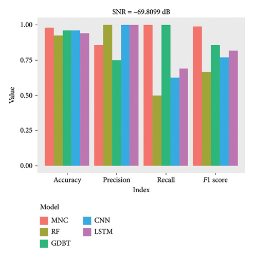
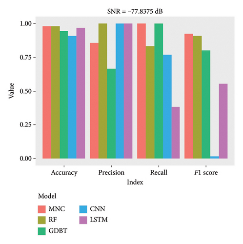
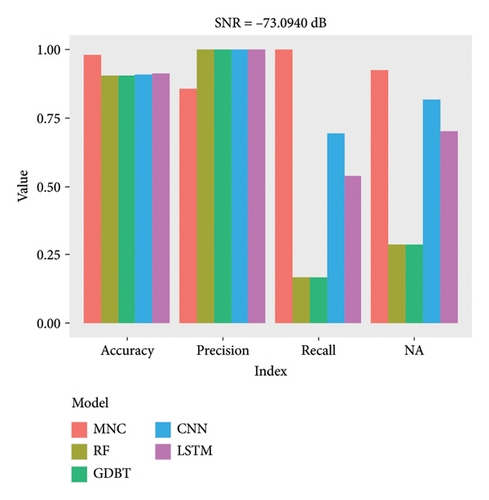
At different signal-to-noise ratios, the accuracy of the MNC function prediction model exceeds that of the other four model methods. Specifically, when the signal-to-noise ratio reaches a certain level, the MNC model achieves higher recall and F1 score compared to the other four models. At another specific signal-to-noise ratio, the accuracy of all four models is similar, with scores of 98.08% for MNC and RF, 96.87% for LSTM, and below 95% for the other models. However, at the third signal-to-noise ratio, the MNC model maintained an accuracy of 98.08%, while the other four models were all below 92%, demonstrating the significant superiority of the MNC model. In summary, when using MNC function prediction models, the performance of multisensor detection fusion is optimal.

It can be observed from Figures 7, 8, and 9 that under different signal-to-noise ratios, the accuracy of the MNC function prediction model is higher than that of the other four model methods, MNC is 98.08%, RF and LSTM have the highest accuracy under the second signal-to-noise ratio, 98.08% and 96.87%, respectively, and the effects of the rest are the worst. GDBT and CNN have the highest accuracy under the first signal-to-noise ratio, 96.15% and 95.85%, respectively. In general, the accuracy of MNC is higher than that of the other four methods. Moreover, when the signal-to-noise ratio reaches a certain level, the MNC model obtains higher recall and F1 scores than the other four models, and the precision of all four models is higher than that of the MNC model, but the difference is not significant. To sum up, when the MNC function prediction model is used, the performance of multisensor detection fusion is the best. The specific reason is that compared with other traditional machine learning models, the MNC model has significant advantages in terms of nonlinear spatio-temporal feature extraction ability and chaos enhancement, as well as the advantages of fusion rules, which makes MNC still perform significantly at different SNRs, not only in terms of accuracy but also in terms of recall and F1 scores.

4.2. Scenario 2: Sea Clutter Experiments and Ablation Study

The sea clutter multidimensional chaotic datasets used in this study comes from the part of IPIX1993 radar data made public by McMaster University, Canada. Due to its open source, the IPIX radar data set is widely used in the detection and characteristic analysis of low observable targets on the sea. The high-resolution echo data of the IPIX radar data set provides valuable measured data support for the detection and characteristic analysis of low observable targets on the sea. Our investigation of this dataset provides critical insights into the intrinsic characteristics of sea clutter, offering foundational support for research in radar signal processing and environmental sensing. While the dataset retains the reference value for chaotic pattern analysis, its utility is partially constrained by historical collection timelines and potential measurement inaccuracies inherent to early-generation instrumentation. Without additional data preprocessing, our comparative analysis in Table 8 demonstrates that the MNC framework consistently outperforms conventional methods (RF, GDBT, CNN, and LSTM) across all evaluation metrics in distributed fusion detection tasks. This performance gap primarily stems from the limited capacity of traditional algorithms to concurrently capture nonlinear spatio-temporal correlations and chaotic enhancement patterns essential for marine environment monitoring. The BLS cascade network emerges as a notable exception, leveraging stochastic mapping mechanisms to preserve chaotic features while enhancing nonlinear feature extraction (a capability explaining its superior detection accuracy over CNN and LSTM architectures). Our proposed MNC-BLS integration systematically combines the strengths of BL paradigms with multivariate correlation modeling, achieving optimal fusion detection through three synergistic mechanisms: (1) distributed correlation preservation across sensor nodes, (2) nonlinear feature hierarchy construction, and (3) chaos-adaptive enhancement. Model robustness is evidenced by consistent performance parity between training and testing phases, effectively mitigating overfitting risks through spatial correlation constraints. This architecture establishes a new paradigm for processing marine chaotic signals without requiring extensive data purification.

Table 8. Detection effects for sea clutter chaotic datasets (SNR = −69.8099 dB).

	Accuracy	Precision	Recall	F1 score
MNC	0.9708	0.8471	0.9670	0.9790
RF	0.9123	0.8123	0.7950	0.8467
GDBT	0.9215	0.7250	0.8012	0.8671
CNN	0.9338	1.0000	0.8667	0.8857
LSTM	0.9523	0.8167	0.9320	0.8890

In our approach, there are three major components: PR, BL, and MNC. To study the effectiveness of our proposed method MNC with PR and BL system, we have some ablation experiments by continuously removing components of our model to observe how the performance degrades on Lorenz and Sea clutter. Firstly, to investigate the feature extraction capability and the effectiveness of feature enhancements of the BL system, we removed the BL system module. Secondly, we remove the PR module for reconstructing the multivariate chaotic attractor and use the output of the BL system directly as input to the MNC network. Table 9 shows the performance result of the ablation studies on sea clutter chaotic datasets, where “×” represents that MNC with the BL system does not adopt or use the component of ∗. Our comprehensive analysis yields three principal conclusions: (i) Enhanced correlation recognition: The integrated MNC architecture incorporating PR and BL components demonstrates superior capability in capturing latent spatial correlations within multivariate chaotic datasets while maintaining high precision in pulse signal detection. This dual functionality addresses critical challenges in processing complex nonlinear systems. (ii) Efficient feature extraction mechanism: The synergistic operation of PR and BL systems enables effective decomposition of reconstructed chaotic structures into interpretable spatio-temporal features, emphasizing their nonlinear and chaotic properties. This methodological innovation not only accelerates feature extraction cycles compared to conventional methods but also facilitates dynamic information reutilization across temporal scales, establishing a new benchmark for real-time processing of high-dimensional chaotic data. (iii) Correlation-preserving architecture: Through rigorous simulation of variable interdependencies in multidimensional chaotic systems, our framework achieves improvement in detection accuracy (F1-score) over baseline models. These results empirically validate that preserving spatial correlations through distributed fusion detection is paramount, with ablation studies confirming that excluding either PR or BL components degrades performance across test scenarios.

Table 9. Ablation study in real chaotic sea clutter datasets.

Method	PR (phase reconstruction)	BL (broad learning)	Accuracy	Precision	Recall	F1 score
MNC	×	×	0.7385	0.7792	0.7854	0.8926
	√	×	0.9387	0.8392	0.9356	0.9391
	×	√	0.9503	0.8201	0.9470	0.9571
	√	√	0.9708	0.8471	0.9670	0.9790

5. Conclusions

The emergence of target signals or faults in sea monitoring or mechanical systems contaminated by a strong chaotic background may discover danger or influence normal operation. We present a novel statistical learning architecture named MNC and apply the BL feature enhancement strategy to finish high accurate weak signal detecting tasks. The PSR is introduced to enable the BL to capture the spatio-temporal feature of the observed 1-D time series signals in distributed sensor networks. The received 1-D signal is reconstructed into fixed-size tuples, and this process is followed by the manifold robust BL embedding. The multiple nonlinear correlation polynomial function is used to link the output of the BL systems with intrinsic information. Additionally, to detect the weak pulse signal from distributed sensor observations, the QRS detector with fusion rules based on the residuals of the MNC model is used to accomplish the detection of the weak pulse signal in chaotic interference by using difference processing, and the detection threshold is calculated according to the difference sequence. The robustness and efficiency of the investigated approach in weak pulse signal fusion detection from distributed sensors under chaotic noise are comprehensively studied by using multiple experiments with different conditions and scenarios for weak pulse signals. We also conduct a comparative analysis. The multiple and comparative results obtained by using different parameters and various methods show that the presented approach achieves higher accuracy, and the proposed method achieves higher accuracy, recall, and F1 score than the RF model, GBDT, CNN, and LSTM models. The proposed MNC model with the BL technique in the reconstructed phase space exhibits a superior ability for feature extracting and fault signal pattern fusion recognition in distributed sensor networks. Additionally, in a comprehensive investigation of an environment involving chaotic additive noise with different SNRs, the proposed approach achieves high detecting accuracy or recall or F1 score. Due to the robustness of the spatio-temporal feature extraction by BL systems with PSR, the MNC model exhibits excellent stability against chaotic interference. The background of this study is twofold: on one hand, experiments were conducted in a chaotic background, and on the other hand, the model detected pulse signals, which did not perform well in other types of signals and backgrounds. This is the limitation of the model proposed in this paper. For the future prospects of the entire model, the methods and applications proposed in this paper can be improved from two aspects. The first aspect is to study how to apply the methods in this paper to other non-Gaussian noise situations or different sensors are interfered by different noises, such as pink noise, or noises with different frequencies. The second aspect is that since we limit the detected signal to pulse signals, we can consider how to generalize it to other types of signals or small target signals, such as harmonic signals or difficult to detect small targets. Additionally, the use of the generalized likelihood ratio can also be considered.

Ethics Statement

The authors have nothing to report.

Disclosure

This paper has been presented as a preprint in the following link: https://assets.researchsquare.com/files/rs-4119174/v1_covered_5fca0a96-d2d2-469f-bc67-10835d1cedf1.pdf?c=1712801739.

The manuscript as a preprint was posted in Research Square. For the detailed information, please see the reference [31].

Conflicts of Interest

The authors declare no conflicts of interest.

Funding

This paper was supported by the Chongqing Natural Science Foundation of China (grant no. CSTB2023NSCQ-MSX0374 and grant no. CSTB2023NSCQ-LZX0048).

Open Research

Data Availability Statement

The data are available on valid request from the corresponding author Liyun Su ([email protected]).

References

All articles

Enhanced Multidimensional Nonlinear Correlation via Phase Reconstruction and Broad Learning for Distributed Fusion Detection of Weak Pulse Signals

Abstract

1. Introduction

1.1. Distributed Structure Universal Detection Fusion System Detection Structure and Current Status

1.2. Introduction to Generalized Learning, Broad Learning (BL), Phase Space Reconstruction (PSR), and Model Structure

1.3. Contribution and Structure of This Article

2. Distributed Signal Detection Problem Under Chaotic Interference

3. Proposed Distributed Detecting Fusion System

3.1. MNC Architecture

3.2. Algorithm Procedure of the Presented Approach

4. Experimental Results and Analysis

4.1. Scenario 1: Simulated Experiments

4.2. Scenario 2: Sea Clutter Experiments and Ablation Study

5. Conclusions

Ethics Statement

Disclosure

Conflicts of Interest

Funding

Open Research

Data Availability Statement

References

Figures

References

Information

About Wiley Online Library

Help & Support

Opportunities

Connect with Wiley

Enhanced Multidimensional Nonlinear Correlation via Phase Reconstruction and Broad Learning for Distributed Fusion Detection of Weak Pulse Signals

Abstract

1. Introduction

1.1. Distributed Structure Universal Detection Fusion System Detection Structure and Current Status

1.2. Introduction to Generalized Learning, Broad Learning (BL), Phase Space Reconstruction (PSR), and Model Structure

1.3. Contribution and Structure of This Article

2. Distributed Signal Detection Problem Under Chaotic Interference

3. Proposed Distributed Detecting Fusion System

3.1. MNC Architecture

3.2. Algorithm Procedure of the Presented Approach

4. Experimental Results and Analysis

4.1. Scenario 1: Simulated Experiments

4.2. Scenario 2: Sea Clutter Experiments and Ablation Study

5. Conclusions

Ethics Statement

Disclosure

Conflicts of Interest

Funding

Open Research

Data Availability Statement

References

Figures

References

Related

Information