MalFSLDF: A Few-Shot Learning-Based Malware Family Detection Framework
Abstract
The evolution of malware has led to the development of increasingly sophisticated evasion techniques, significantly escalating the challenges for researchers in obtaining and labeling new instances for analysis. Conventional deep learning detection approaches struggle to identify new malware variants with limited sample availability. Recently, researchers have proposed few-shot detection models to address the above issues. However, existing studies predominantly focus on model-level improvements, overlooking the potential of domain adaptation to leverage the unique characteristics of malware. Motivated by these challenges, we propose a few-shot learning-based malware family detection framework (MalFSLDF). We introduce a novel method for malware representation using structural features and a feature fusion strategy. Specifically, our framework employs contrastive learning to capture the unique textural features of malware families, enhancing the identification capability for novel malware variants. In addition, we integrate entropy graphs (EGs) and gray-level co-occurrence matrices (GLCMs) into the feature fusion strategy to enrich sample representations and mitigate information loss. Furthermore, a domain alignment strategy is proposed to adjust the feature distribution of samples from new classes, enhancing the model’s generalization performance. Finally, comprehensive evaluations of the MaleVis and BIG-2015 datasets show significant performance improvements in both 5-way 1-shot and 5-way 5-shot scenarios, demonstrating the effectiveness of the proposed framework.
1. Introduction
The exponential growth of malware poses a significant threat to cybersecurity. According to a recent AV-TEST report [1], more than 307,000 new malware samples are generated daily, including numerous newly evolved malware families. This issue is further exacerbated by the increasing complexity of modern computing environments, where diverse devices and systems are interconnected. Many devices, particularly those with limited computational resources and inadequate security measures, are highly vulnerable to malware attacks. Therefore, accurate malware detection is critical for ensuring robust cybersecurity.
Traditional malware detection methodologies predominantly employ static, dynamic, and hybrid analyses techniques to extract discriminative features from samples, which are subsequently classified utilizing machine learning or deep learning models [2]. Nevertheless, static analysis is inherently limited by its vulnerability to obfuscation techniques, including packing and encryption, whereas dynamic analysis demands substantial computational resources and time. Recent advances in visualization-based classification [3, 4] have introduced a novel paradigm by converting malware binaries into visual representations, enabling direct analysis through neural networks. The visualization-based approach [5] not only simplifies the classification processes but also circumvents many limitations associated with traditional methods. However, many detection models [6–9] require large-scale datasets to achieve high accuracy, which is often impractical given the limited availability of labeled malware samples. This situation exemplifies the few-shot learning (FSL) problem and is a key challenge in modern malware detection.
FSL, as outlined in research [10], addresses data scarcity by leveraging prior knowledge, such as domain expertise or data from related tasks, and employs techniques such as data augmentation, model regularization, and pretraining followed by fine-tuning to enhance classification performance. Current FSL approaches focus on three key components: data, models, and algorithms [11]. Data augmentation methods, including translation, flipping, cropping, and rotation, as well as advanced techniques such as label propagation [12] and generative adversarial networks (GANs) [13], are commonly used to generate synthetic samples. Transfer learning approaches [14] train models on a source domain with abundant labeled data, using learned model parameters or features as prior knowledge to initialize and fine-tune the model in a target domain with limited labeled data. Algorithmic limitations are mainly addressed using meta-learning approaches [15] involving feature parameter optimization, model architecture refinement, and similarity measurement techniques. In malware family classification, FSL can extract essential feature patterns from labeled datasets and apply them to small sets of newly captured malware, facilitating feature extraction and the classification of new malware samples into corresponding families [16–19].
Despite significant advancements in FSL methods, several limitations persist that impede their effectiveness in malware detection. First, many commonly used FSL data augmentation methods face domain misadaptation issues in the malware field. For instance, flipping, cropping, rotation, and mixup often compromise the semantic coherence of malware grayscale images [20]. This distortion obscures critical family-specific patterns, undermining the model’s ability to discern discriminative features and resulting in suboptimal classification performance. Moreover, existing data preprocessing techniques that standardize sample sizes frequently lead to the loss of critical information, thereby impairing the model’s capacity to capture and learn intrinsic data characteristics. Furthermore, existing meta-learning–based FSL methods typically assume that the distribution of pretraining samples with known labels aligns with that of new class samples [21, 22]. This assumption, known as distribution consistency, often fails in practical applications, especially in few-shot malware classification, where the distribution of new class samples is unknown in advance. These issues collectively degrade the generalization performance of FSL methods.
To solve the abovementioned questions, we propose a few-shot learning-based malware family detection framework (MalFSLDF). Specifically, our approach addresses domain misadaptation by introducing a novel method for malware representation using structural features and a feature fusion strategy. We propose a contrastive learning (CL)–based feature extraction method for malware grayscale images under few-shot conditions. We also employ augmentation techniques such as Gaussian blur to retain semantic information while improving the model’s ability to identify malware variants. In addition, we introduce a multifeature construction and fusion strategy to mitigate information loss during data processing, extracting features such as entropy graphs (EGs) and gray-level co-occurrence matrices (GLCMs) from original malware grayscale images. These features are fused with representations obtained through CL, enriching the information of the samples and facilitating the model’s ability to capture the salient characteristics of malware. Finally, we propose a domain alignment (DA) method to address distribution inconsistency. This method adjusts the feature distribution of new class malware samples to align with that of known samples from the training set, thereby improving the model’s generalization performance.
- •
We propose a novel few-shot visualization-based malware family detection framework, MalFSLDF, which improves existing FSL methods by incorporating malware-specific enhancements in data augmentation and malware representation, thus achieving efficient few-shot malware detection.
- •
We propose a novel malware representation method based on structural features. Specifically, we employ CL to extract the texture features of malware grayscale images and integrate GLCM and EG through a feature fusion strategy, achieving a comprehensive representation of malware samples.
- •
We utilize a DA strategy to adjust the feature distribution of samples from new classes, thereby enhancing the model’s generalization performance.
- •
Comprehensive evaluations on the MaleVis and BIG-2015 datasets demonstrate significant performance improvements in both 5-way 1-shot and 5-way 5-shot scenarios, validating the effectiveness of the proposed framework.
The rest of this paper is organized as follows. Section 2 summarizes related work. Section 3 provides preliminaries and problem formulas. Section 4 details the proposed method. Section 5 presents experimental results. Section 6 presents the discussion of the study. Section 7 concludes the study and discusses future work.
2. Related Work
2.1. Visualization-Based Malware Detection
Traditional malware detection methods utilize static, dynamic, or hybrid analysis techniques to extract features, applying deep learning or machine learning models to classify malware families. Detection techniques that rely on dynamic and static analyses depend heavily on known behavioral patterns, making it challenging to detect variants of malware with unique behaviors. In contrast, visual techniques provide an advantage by transforming complex patterns into visual representations. This allows for quick and effective identification of various malware patterns, making them particularly useful for detecting malware variants.
Nataraj et al. [5] pioneered research in this domain by observing that malware grayscale images from the same family share similar layouts and textures. Based on these visual similarities, they proposed an image-based method for malware family classification. Xiao et al. [23] introduced colored label boxes (CoLabs) to mark different segments of PE files, highlighting the distribution of certain parts within transformed malware images. Jeon et al. [6] used Shannon entropy to detect obfuscation, followed by dynamic analysis to extract application programming interface (API) call sequences, which were converted into images for detection. Later, they proposed Mal3S [7], extracting bytes, opcodes, API calls, strings, and dynamic-link libraries (DLLs) via static analysis to generate five image types, trained with a Multi–SPP-net model for malware detection.
Sharma et al. [8] introduced MIGAN, a GAN–based model, to address class imbalance by generating high-quality synthetic malware images, achieving strong classification performance. Vasan et al. [24] combined visualization, feature decomposition, and broad learning systems to improve malware detection, leveraging random vector functional link neural networks for enhanced classification. He et al. [25] developed an attention mechanism based on the ResNeXt model, improving classification accuracy by capturing channel-specific fields in malware images. Research [26] extracted features from assembly files, converting them into binary form and creating images from the generated binary representation. Zhong et al. [9] proposed a method that utilizes self-similarity techniques to extract local semantics and similarities within binary malware blocks while maintaining correlations between these blocks. Zhang et al. [27] designed a deep polarized network based on ResNet50, maximizing the Hamming distance between hash values of malware samples from different families.
In summary, existing research demonstrates technical strengths in image processing, feature extraction, and model algorithms. However, significant challenges persist, including high computational resource demands, processing complexity, and limited scalability, particularly when addressing obfuscated malware. In addition, deep learning models rely heavily on large labeled datasets for effective classifier training, raising concerns about overfitting with limited labeled samples. Therefore, this research focuses on malware detection in few-shot scenarios.
2.2. Few-Shot Malware Detection
Most existing few-shot malware detection research directly employs classical FSL methods [28–30], such as prototypical networks (ProtoNets) [16], matching networks [17], Siamese networks [18], and memory-augmented networks. However, these methods lack generalizability, showing inconsistent performance across different datasets.
Some recent approaches combine various data augmentation and meta-learning techniques. Chai et al. [21] proposed a dynamic prototype network based on sample adaptation, using dynamic convolution for sample-adaptive dynamic feature extraction. Class features (prototypes) are defined as the mean of dynamically embedded malware samples in the support set. The method also introduces a dual-sample dynamic activation function to minimize the impact of irrelevant features between samples, and a metric-based approach calculates the distance between query samples and prototypes for malware detection. Conti et al. [19] introduced a few-shot malware classification method utilizing malware feature visualization, representing malware binaries as three-channel images. They employed convolutional Siamese neural networks and shallow FSL architectures to address the retraining issues of traditional deep learning classifiers.
Barros et al. [22] proposed Malware-SMELL, which incorporates two data representation spaces: latent feature space and similarity space (S-Space). In S-Space, a kernel-based discrete Cauchy distribution is used to quantify the similarity between input pairs, measuring the distance between labels and new data representations to address the challenges of the FSL paradigm. Liu et al. [31] proposed A2-CLM, a self-supervised malware detection framework that integrates adversarial heterogeneous graph augmentation with CL. By evaluating the security semantics of each behavior, A2-CLM constructs a heterogeneous graph of malware execution contexts. Multiple adversarial attacks, including attribute masking attacks, meta-graph–guided sampling attacks, direct system call attacks, and obfuscation attacks, are designed to generate more robust contrastive pairs. In addition, a momentum strategy is proposed to train multiple graph encoders, mitigating the workload associated with CL.
In summary, current few-shot malware detection methods still face several limitations. First, existing approaches necessitate extensive feature engineering and substantial expert knowledge. Second, conventional FSL techniques that are not directly applicable to malware detection may disrupt the texture features of malware samples, leading to confusion, introducing noise, and reducing model accuracy. Furthermore, most model improvement strategies do not adapt to the unique characteristics of malware, leading to inconsistent performance across datasets and limited generalization capabilities. Hence, this study proposes enhancements in data augmentation, parameter optimization, and similarity measurement.
3. Preliminaries and Problem Formulas
3.1. Processing of the Malware Grayscale Image
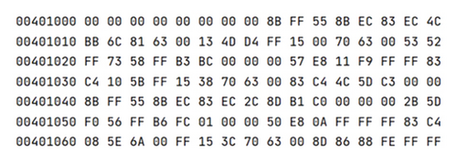
This section presents the conversion of source binary malware files into grayscale images. As shown in Figure 1, the original binary file is stored in byte format, with the data starting address on the left side of each line in 8 bits and the file content represented in hexadecimal on the right.
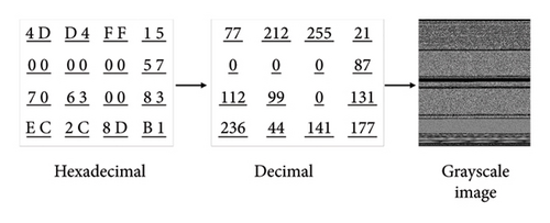
The process of converting bytecode to grayscale images is depicted in Figure 2. Specifically, hexadecimal numbers are initially converted to binary numbers, subsequently grouped into 8-bit vectors, and then transformed into decimal integers within the range of 0–255. This process generates a grayscale image, where 0 corresponds to black and 255 corresponds to white.
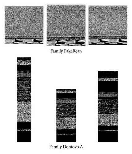
As illustrated in Figure 3, malware samples from the same family appear visually similar in grayscale images, whereas those from different families are distinct. This phenomenon is due to the reuse of malware construction patterns within families, with minimal changes to texture features. Thus, image classification can effectively distinguish malware categories based on grayscale images.
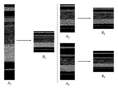
In addition, grayscale malware images must be standardized to be adapted for neural network analysis. Motivated by the work [32], this study uses bilinear interpolation to resize images to 224 × 224 pixels, which optimally preserves texture features. Figure 4 shows the transformation effect of the Dontovo family images, where A1, A2, and A3 are the original images with sizes of 64 × 456, 128 × 244, and 128 × 320, respectively, and B1, B2, and B3 are the corresponding transformed grayscale images, all with a size of 224 × 224.
3.2. CL
CL is a critical form of self-supervised learning, which learns effective data representations by constructing and comparing positive and negative sample pairs. Positive samples are typically different views or augmented versions of the same data, whereas negative samples come from views of different data points. The training objective is to bring positive samples closer in the feature space while pushing negative samples further apart. This method enables the model to learn features that differentiate between categories, allowing it to acquire useful data representations without labeled data.
Specifically, for each original image x, two augmented samples xi and xj are generated, and a neural network, such as a convolutional neural network, is used as an encoder f to encode the two augmented samples into corresponding feature representations hi and hj. Further projection layers enhance the quality of these learned features, producing more compact and discriminative feature representations. Contrastive loss ensures that the representations of the two augmented samples are close in the feature space. This approach does not require label information and relies entirely on the intrinsic structure of the input data to learn meaningful representations.
3.3. Problem Formula
In traditional deep learning frameworks, datasets are divided into training and test sets, which share the same category space. However, in FSL scenarios, the training and test sets contain different category spaces. The test set is further divided into support and query sets, which share a common category space. As shown in Figure 5, different colored squares represent different malware families.
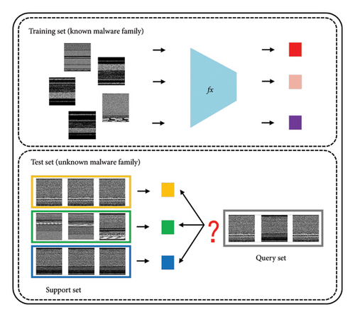
The core of FSL lies in using a large labeled training set and a small labeled support set to classify unlabeled query samples. In the context of malware classification, the training set consists of malware samples from known categories. In contrast, the support set of the test set includes a small number of new category samples, and the query set contains the new samples to be classified.
First, the model learns transferable knowledge from the training set, such as a feature extraction method fx, and then leverages this knowledge to extract features from new test samples. It combines the small sample set in the support set (S) and their labels to classify the samples in the query set (Q). In typical FSL settings, if the support set consists of N categories and K samples per category, this is called an N-way K-shot problem. Generally, N and K are small values, reflecting the nature of FSL, where the model must recognize N categories based on a limited set of N∗K samples.
In deep learning, classification tasks are typically approached with two learning paradigms: inductive learning and transductive learning. Inductive learning focuses on constructing and training models from training datasets to achieve effective generalization on unseen test data. Conversely, transductive learning leverages the distributional information of test data during training, providing additional guidance to the model despite the absence of labels, but necessitates continuous model updates with new samples. Considering the unpredictability of malware categories and their distribution, coupled with the resource expenditure associated with frequent model updates, this study posits that inductive learning is more suitable for classifying malware.
4. Methodology
4.1. Overview of MalFSLDF
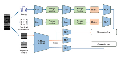
To address the challenges of malware family classification in few-shot scenarios, this paper introduces MalFSLDF. As shown in Figure 6, MalFSLDF comprises four core modules: feature extraction, feature fusion, DA, and classification, each serving as a key component for effective malware detection.
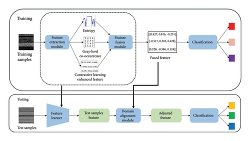
Feature Extraction Module. This module focuses on processing grayscale images of malware, generating a richer representation by profiling malware from multiple dimensions. A CL method tailored for malware is proposed, which enhances the family level feature representation of grayscale images. The original grayscale images’ EG and GLCM are also constructed as auxiliary features.
Feature Fusion Module. This module assigns weights to the three types of features extracted from the feature extraction module, ensuring that the model captures the family level traits of malware samples comprehensively. In addition, a custom loss function is designed to allow backpropagation of feature loss, optimizing the backbone network and generating more accurate feature representations.
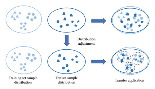
DA Module. This module addresses the distribution mismatch between training and test samples, ensuring that knowledge extracted from the source domain can be transferred effectively to the target domain. A feature mapping approach is introduced to assess the correlation between test sample features and the prototype features from the training samples, reducing the gap between their feature distributions.
Classification Module. This module begins by extracting the class mean feature representations of the support set samples. Then, it calculates the distance between the query sample features and the class centers in the support set. Each query sample is classified based on proximity to the nearest class center.
4.2. CL Enhanced Feature Extraction
In order to preserve the texture features of malware grayscale images, this paper introduces a novel data augmentation strategy, which leverages Gaussian blur and noise injection to generate high-quality samples essential for CL. Specifically, a CL branch is added to the backbone network to capture the features of malware family samples. This enhances the accuracy of feature representations, thereby improving the overall performance of the system.
4.2.1. Data Augmentation Strategy
In order to preserve the texture features of malware grayscale images, this paper introduces a novel data augmentation strategy, which leverages Gaussian blur and noise injection to generate high-quality samples essential for CL. Specifically, three enhancement techniques are utilized: horizontal flipping, color jittering, and Gaussian blur. Horizontal flipping preserves the vertical texture patterns of the original images.
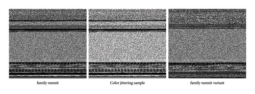
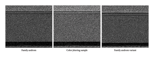
Color jittering is a data augmentation technique characterized by stochastic adjustments to brightness and contrast [33, 34]. Malware variants often exhibit minor payload alterations, such as instruction modifications or the addition/removal of functional modules, which manifest as subtle variations in pixel intensity within grayscale image representations. By applying color jittering, we simulate these pixel-level changes, enhancing the model’s ability to generalize across different malware instances with similar structures but slight differences. Figure 7 illustrates examples of color jittering, featuring a 50% increase in both brightness and contrast, using samples from the Ramnit and Androm families in the BIG-2015 and MaleVis datasets. These examples demonstrate that color jittering induces subtle changes in pixel intensity, reflecting the minor payload modifications observed in malware variants, while preserving the overall structural integrity of the grayscale representation.
Furthermore, Gaussian blur reduces image noise by applying a Gaussian filter, helping the model focus more on the overall structure of the image rather than on fine details. This allows the model to handle images of varying quality in real-world scenarios, reduces reliance on high-quality images, lowers the risk of overfitting, and improves model performance during testing.
The Gaussian blur implementation is outlined in Algorithm 1. The core computation employs a convolution operation where each pixel’s blurred value derives from a Gaussian-weighted summation of its neighbors. We first initialize a zero matrix of the same size I according to the size of each malware image. With each pixel (x, y) in the original image as the center, the Gaussian weight of the neighborhood of k × k is calculated according to the standard deviation σ, and the Gaussian weight is multiplied and summed with the pixels in the corresponding position in the neighborhood and the pixel value I′(x, y) after fuzzy processing is obtained.
-
Algorithm 1: Gaussian blur algorithm implementation.
-
Require:I: Original image, k: size of the Gaussian kernel, σ: standard deviation
-
Ensure:I′: Blurred image
- 1.
image_size ← I.size( )
- 2.
I′ ← zero_array(image_size)
- 3.
for(x, y) ∈ Ido
- 4.
temp ← 0
- 5.
for(i, j) ∈ [−(k/2), k/2] × [−(k/2), k/2]do
- 6.
w ← (1/(2πσ2))exp(−(i2 + j2)/(2σ2))
- 7.
if(x + i, y + j) ∈ Ithen
- 8.
temp ← temp + w × I(x + i, y + j)
- 9.
end if
- 10.
end for
- 11.
I′(x, y) ← temp
- 12.
end for
- 13.
returnI′
Specifically, boundary regions require special treatment as incomplete neighborhoods disrupt standard convolution. First, a mirroring technique is employed, where the pixels near the boundary are reflected, creating a virtual extension of the image. This process ensures that the Gaussian filter has neighboring pixels to perform the convolution. Second, the edge pixels are handled by adjusting the weight distribution to minimize the impact of missing neighbors, ensuring that the boundary areas are smoothly blurred without introducing artificial artifacts. These mechanisms ensure artifact-free blurring across all image regions while maintaining the Gaussian kernel’s mathematical integrity.
4.2.2. Design of the CL Network
Pretext tasks such as rotation and crop prediction in classical CL are ineffective for malware classification because they disrupt key texture features in grayscale images, resulting in unstable feature representations. To address these limitations, we propose a novel CL network architecture that incorporates both supervised and unsupervised learning. The network architecture and layer-specific parameters are illustrated in Figure 8. ResNet12 [35] is adopted as the backbone architecture. Specifically, a classification head, structurally identical to the projection head, is added at the same hierarchical level.
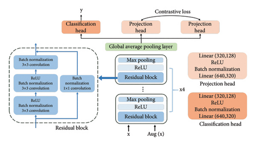
Consistent with classical methods, the projection head maps features extracted by the backbone network into a lower-dimensional space, enabling the accurate measurement of similarities and differences between samples. In addition, the classification head leverages limited malware category labels for supervised learning, enhancing the model’s ability to capture structural features and improve classification performance. In addition, unlike conventional CL that relies on two augmented samples as inputs, our method incorporates the original sample as one of the inputs. This configuration not only more accurately reflects the structural characteristics of the real samples but also allows for the utilization of original sample labels for supervised learning.
The proposed network facilitates the simultaneous execution of CL and classification tasks. The projection head conducts CL by maximizing the contrastive loss between different samples while minimizing it for identical sample pairs, thereby optimizing feature representations. Furthermore, the classification head enhances the model’s capability for classification by minimizing the classification loss. This approach empowers the model to develop more comprehensive and robust feature representations.
4.2.3. Design of the Loss Function
In CL, the objective is to minimize the distance between similar samples and maximize the distance between dissimilar ones. In practice, augmented variants of the same sample are considered positive pairs due to their semantic consistency. Conversely, negative pairs are constructed from other samples within the same batch, as these samples typically belong to different classes and thus provide effective contrast.
4.3. Malware Multifeature Fusion (MF) Module
To learn richer feature representations of malware, the multifeature construction and fusion process is introduced. This process includes EG generation, GLCM calculation, and feature fusion.
4.3.1. Construction of Malware EG
Malware commonly employs packing and compression techniques to conceal its true structure and functionality, complicating static analysis and evading detection by security mechanisms. Compared to benign code, packed and compressed sections typically exhibit higher entropy values, making entropy analysis an effective tool for rapidly identifying packed and encrypted malware samples.
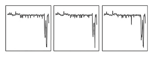
The process of constructing the EG of a grayscale image consists of three steps: first, segmenting the original malware grayscale image, then calculating the information entropy for each segment using Shannon’s formula, and finally, plotting the calculated entropy values as a line graph, which results in the EG.
To ensure comparability of the EGs, the map’s height is fixed to correspond to the maximum possible entropy when all grayscale values occur with equal probability.
As shown in Figure 9, EGs derived from the same malware family display a high degree of similarity, whereas those from distinct families exhibit clear differences.

4.3.2. Construction of GLCM
Malware grayscale images exhibit distinct vertical texture features, and common texture feature extraction algorithms include GLCM, local binary pattern, and Gabor transform [37]. GLCM has the lowest computational complexity, making it an ideal choice for this paper as an auxiliary feature for malware grayscale images.
-
Algorithm 2: GLCM construction.
-
Required:Igray: Grayscale image, Levels: number of quantized gray levels, Distance: distance parameter, Direction: direction parameter
-
Ensure:GLCM, Features
- 1.
Levels_before = max(Igray) + 1
- 2.
R = (Levels/Levels_before) = L″/L
- 3.
for(x, y) ∈ Igraydo
- 4.
gray1 = Igray(x, y)
- 5.
Igray(x, y) = R·gray1
- 6.
end for
- 7.
GLCM = np.zeros(Levels, Levels)
- 8.
for(x, y) ∈ Igraydo
- 9.
gray1 = Igray(x, y)
- 10.
Use Distance and Direction to find (x′, y′)
- 11.
gray2 = Igray(x′, y′)
- 12.
GLCM(gray1, gray2) = GLCM(gray1, gray2) + 1
- 13.
end for
- 14.
Calculate Features of GLCM
- 15.
returnGLCM, Features
As shown in Algorithm 2, the construction of GLCM involves three main steps: grayscale compression, co-occurrence matrix generation, and feature computation. First, pixel values are extracted from the grayscale image to form a grayscale matrix, and grayscale compression is applied to the original matrix to reduce dimensionality and computational load. If the original grayscale level is L and the target level is L″, then the compression ratio R is L″/L. Each pixel in the original image is multiplied by the compression ratio and rounded down to obtain the compressed grayscale value. Next, adjacent pixels are identified in the compressed image using a defined direction and distance. The grayscale levels of the current and adjacent pixels are used as indices to update the co-occurrence matrix. For instance, if the grayscale level of the current pixel is i and the adjacent pixel is j, the value at position (i, j) in the co-occurrence matrix is incremented by 1. Considering the substantial manual effort required for feature selection when employing these metrics, this paper will utilize the GLCM derived directly from the original grayscale levels for model training. The neural network automatically captures the latent features within the GLCM. Since the initial grayscale level is 256, the size of the GLCM is set to 256 × 256.
4.3.3. Fusion of Multifeature
This paper integrates EGs and GLCM of malware grayscale images as auxiliary features to construct a feature fusion network, producing fused feature representations that enhance classification performance.
4.4. DA–Based Feature Distribution Adjustment Strategy
This paper introduces a feature mapping–driven DA strategy that aims to adjust the distribution of test data during the testing phase to align it more closely with the training data distribution, thereby improving the classification accuracy of test data.
After adjusting the feature distribution, the feature representations of the test sample align closely with the distribution of the training samples. Spatially, this manifests as the test samples clustering around the training prototypes, as depicted in Figure 11.
5. Evaluation
5.1. Experimental Settings
5.1.1. Dataset
This study evaluates the model on two publicly accessible Windows malware datasets: MaleVis [42] and BIG-2015 [43]. MaleVis contains 26 categories (1 benign and 25 malware families) with RGB images of 224 × 224 and 300 × 300 resolutions, comprising 9100 training and 5126 validation images. A balanced subset of 25 malware classes is used for evaluation, partitioned by the FSL method into 15 training, 5 validation, and 5 testing classes. BIG-2015, released by Microsoft, contains 21,741 samples from 9 malware families, with 10,868 labeled and 10,873 unlabeled samples. Due to imbalanced sample distribution, this study focuses on four categories, Ramnit, Lollipop, Kelihos_Ver3, and Gatak, as the training set, while the remaining five categories are reserved for the test set.
Baseline models (BLs) and improved approaches are applied to both the MaleVis and BIG-2015 datasets to validate their effectiveness. Since the MaleVis dataset comprises RGB images, they are treated as three overlapping grayscale images, and the model’s input channels are adjusted from 1 to 3 to handle the RGB format. As for the BIG-2015 dataset, bilinear interpolation is used to standardize the sizes of samples, and random or oversampling is employed to balance the number of samples in each category to 500, thereby mitigating the effects of data imbalance on the final results.
5.1.2. Experimental Setup
This study divides the dataset into training, validation, and test sets. The validation set is used to assess the model’s generalization performance, and the model achieving the highest validation accuracy is preserved for final testing. Training is set to a default of 300 epochs, and early stopping is triggered if validation accuracy ceases to improve after 50 epochs to prevent overfitting. The batch size is set to 12 during training, and the stochastic gradient descent (SGD) optimizer is employed with an initial learning rate of 0.1. Cosine annealing is used to dynamically adjust the learning rate, preventing improper learning rate adjustments. During testing, 15 samples are queried each time, and the process is repeated 10,000 times, with the average taken as the final evaluation result.
5.1.3. Few-Shot Scenarios and Evaluation Metrics
This paper employs classification accuracy in 5-way 1-shot and 5-way 5-shot scenarios as the primary evaluation metrics. In a 5-way 5-shot task, each class has 5 training samples, whereas, in a 5-way 1-shot task, each class has only 1 training sample. These evaluation approaches effectively reflect the model’s generalization and learning capacity in limited data.
The malware family classification problem addressed in this paper, designed for FSL, is a multiclass classification problem, so standard multiclass evaluation metrics such as precision, recall, and F1-score are considered.
5.2. Results and Analysis
5.2.1. Comparison With Other Works
To verify the performance of MalFSLDF, we select several state-of-the-art works as the BLs and make a comprehensive comparison during the experiments.
5.2.1.1. BLs
ProtoNet [38] introduced a method that leverages the feature representations of a small number of samples in the support set, calculating the mean feature representation of each class for classification. New query samples are categorized based on the similarity or distance between their features and the prototypes of each class.
Relation network (RN) [39] designed an embedding module that embeds samples into a low-dimensional feature space to extract their deep feature representations. A few-shot classification is accomplished by comparing the deep nonlinear distance metrics between query samples and support set samples calculated by the relation module.
RFS [40] trained a high-performance feature extractor on a large-scale dataset to obtain robust embedded representations. These pretrained embeddings are employed directly for few-shot classification, eliminating the need for additional adjustments.
DeepEMD [41] partitioned images into multiple patches and introduced earth mover’s distance (EMD) as a novel metric to calculate the optimal matching flow between patches in the query and support set images. Classification is performed by comparing the similarity of different local regions within the images.
DeepBDC [32] used neural networks to learn the embedded features of samples, calculating the Brownian distance covariance (BDC) distance between these features to measure dependencies among samples, thereby capturing subtle distinctions between them.
EASY [20] enhanced the initial samples using a feature generator, generating diversified virtual samples to augment the training data. An adaptive feature aggregation mechanism effectively merges the feature information from both original and augmented samples, improving the model’s generalization capabilities.
5.2.1.2. Comparison With BLs
This study evaluates the classification performance of existing models and the proposed MalFSLDF on the MaleVis and BIG-2015 datasets under the 5-way 1-shot and 5-way 5-shot configurations. As shown in Table 1, the MalFSLDF framework achieves a significant enhancement in accuracy, ranging from an increase of 4.71% to 14.31% in the 5-way 1-shot classification paradigm and from 4.47% to 19.3% in the 5-way 5-shot classification paradigm. The comparative experimental results across both datasets confirm the effectiveness of the MalFSLDF, which outperforms BLs and demonstrates strong generalization capability.
| Models | MaleVis | BIG-2015 | ||||||||||||||
|---|---|---|---|---|---|---|---|---|---|---|---|---|---|---|---|---|
| 5-way 1-shot | 5-way 5-shot | 5-way 1-shot | 5-way 5-shot | |||||||||||||
| Acc | Pre | Rec | F1 | Acc | Pre | Rec | F1 | Acc | Pre | Rec | F1 | Acc | Pre | Rec | F1 | |
| ProtoNet [38] | 65.39 | 66.71 | 65.39 | 66.04 | 68.72 | 70.55 | 68.72 | 69.63 | 55.44 | 57.54 | 55.44 | 56.47 | 62.85 | 64.83 | 62.85 | 63.82 |
| RN [39] | 59.95 | 59.07 | 59.95 | 59.51 | 66.31 | 65.98 | 66.31 | 66.14 | 54.98 | 50.37 | 54.98 | 52.23 | 61.14 | 56.17 | 61.14 | 58.26 |
| RFS [40] | 68.88 | 70.81 | 68.88 | 69.83 | 73.69 | 75.07 | 73.69 | 74.38 | 50.35 | 53.50 | 50.35 | 51.64 | 65.42 | 67.77 | 65.42 | 66.54 |
| DeepEMD [41] | 67.94 | 69.91 | 67.94 | 68.91 | 71.47 | 73.42 | 71.47 | 72.43 | 51.27 | 52.46 | 51.27 | 51.86 | 66.18 | 67.32 | 66.18 | 66.75 |
| DeepBDC [32] | 68.75 | 70.74 | 68.75 | 69.73 | 72.90 | 74.95 | 72.90 | 73.91 | 52.40 | 55.33 | 55.33 | 53.63 | 68.14 | 70.19 | 68.14 | 69.15 |
| EASY [20] | 65.19 | 65.92 | 65.19 | 65.55 | 69.25 | 70.67 | 69.25 | 69.96 | 56.43 | 53.73 | 56.43 | 54.68 | 67.53 | 69.79 | 67.53 | 68.61 |
| MalFSLDF | 74.26 | 74.29 | 74.26 | 74.27 | 87.56 | 87.63 | 87.56 | 87.52 | 64.33 | 64.57 | 64.33 | 64.45 | 73.92 | 73.97 | 73.92 | 73.94 |
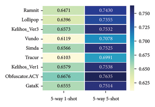
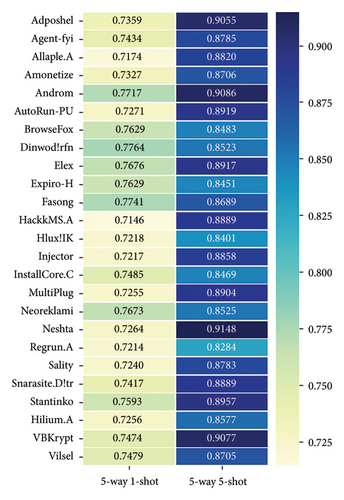
The classification accuracies of malware families in the BIG-2015 and MaleVis datasets under various few-shot settings are shown in Figures 12 and 13, respectively. It is observed that the performance under the 5-way 5-shot setting is markedly superior to that under the 5-way 1-shot setting. In addition, it is noted that the classification performance for some families is comparatively poor. This phenomenon can be attributed to the fact that these families are categorized within the same category, which induces similarity in their grayscale image texture features. For instance, in the BIG-2015 dataset, both “Vundo” and “Tracur” are categorized as Trojans, and in the MaleVis dataset, both “Allaple.A” and “Hlux!IK” are classified as worms.
By introducing a CL module, the model proposed in this paper is capable of effectively capturing the texture features of malicious sample images, thereby achieving a more accurate preliminary representation of their global structural features. Unlike traditional methods such as ProtoNet and RN, which rely solely on single-scale feature matching, and the RFS method that uses only single-view pretrained features, the MF mechanism proposed in this paper captures more complementary information from multiple analytical perspectives, thus achieving a comprehensive representation of the structural information of malicious samples. This multidimensional feature fusion significantly enhances the model’s ability to recognize complex samples. In addition, the sample augmentation strategy proposed in this paper, compared to traditional feature generation methods such as EASY, avoids disrupting the structural information embedded in malicious sample images. This strategy generates effective sample variants while preserving the original structural features of the samples, thereby enhancing the model’s learning ability in data-scarce situations and making it more suitable for malicious code detection tasks. Compared to traditional methods such as DeepEMD and DeepBDC, which rely on fixed distance metrics for sample matching, the dynamic feature adaptation mechanism based on DA proposed in this paper adjusts the features of detected samples dynamically according to the feature distribution of known samples.
Khan et al. [44] developed a RN–based framework for FSL malware detection, comprising a discriminative feature extractor for grayscale images and a relation module for similarity assessment. Our approach presents three fundamental advancements: First, our feature fusion strategy generates more robust feature representations compared to their raw grayscale feature construction. Second, our model incorporates DA to dynamically characterize test sample features for malware classification. Third, while their work focuses on binary detection, our framework addresses the more challenging task of multifamily classification.
Notably, our proposed model exhibits real-time processing capabilities. On the one hand, our approach directly converts binary malware bytecode into grayscale images for feature extraction and detection, eliminating the need for static or dynamic analysis processes. This approach significantly improves processing efficiency while reducing latency. Moreover, our proposed model’s inductive learning mechanism provides enhanced generalization capability, enabling effective handling of emerging novel samples in evolving malware scenarios.
5.2.2. Effectiveness of CL
This study evaluates the effectiveness of an improvement strategy based on CL. In this context, the BL is represented as BL, and CL is represented as CL.
Table 2 illustrates that on the MaleVis dataset, the CL–based improvement strategy significantly enhances classification accuracy compared to the BL. In the 5-way 1-shot setting, the improvement achieved a 3.11% increase in accuracy, and in the 5-way 5-shot setting, the improvement margin was 1.29%. These outcomes demonstrate the effectiveness of contrastive learning–based improvements, particularly in accurately classifying unlabeled samples when each class has only one labeled example.
| Method | MaleVis dataset | BIG-2015 dataset | ||||||||||||||
|---|---|---|---|---|---|---|---|---|---|---|---|---|---|---|---|---|
| 5-way 1-shot | 5-way 5-shot | 5-way 1-shot | 5-way 5-shot | |||||||||||||
| Acc | Pre | Rec | F1 | Acc | Pre | Rec | F1 | Acc | Pre | Rec | F1 | Acc | Pre | Rec | F1 | |
| Baseline (BL) | 69.55 | 69.71 | 69.55 | 69.63 | 83.09 | 83.19 | 83.09 | 83.14 | 56.43 | 53.73 | 56.43 | 54.68 | 67.53 | 69.79 | 67.53 | 68.61 |
| Contrastive learning (CL) | 72.66 | 72.79 | 72.66 | 72.72 | 84.38 | 84.47 | 84.38 | 84.43 | 60.77 | 61.04 | 60.77 | 60.91 | 70.61 | 70.65 | 70.61 | 70.63 |
Table 2 also presents the experimental results for the BIG-2015 dataset. Since this dataset relies on the disassembly tool IDApro to generate hexadecimal values converted into grayscale images, it contains many unknown values, resulting in a decrease in classification accuracy. Nevertheless, the CL–based improvement strategy outperforms the BL across all metrics. Notably, in the 5-way 1-shot configuration, the improvement strategy’s precision exceeds that of the BL by 7.31%, underscoring its low misclassification rate when accurately identifying specific malware categories.
5.2.3. Effectiveness of MF
This work proposes an improved approach based on multifeature construction and fusion at the data level. Specifically, two feature fusion strategies are presented: The first strategy employs a separate network structure to process the EG and GLCM, and the features are fused by optimizing the total loss via backpropagation. The baseline strategy directly concatenates these two features with CL representations, followed by classification using a multilayer perceptron.
As shown in Table 3, it is evident that adding the EG alone significantly boosts the model’s classification accuracy; performance is further improved by incorporating the GLCM. Specifically, in the MaleVis dataset, the classification accuracy increased by 1.77% and 2.69% in the 5-way 1-shot and 5-way 5-shot settings, respectively. On the BIG-2015 dataset, the accuracy increased by 4.86% and 3.22% under the same configurations. Moreover, the fusion strategy demonstrated a more notable effect on the BIG-2015 dataset, particularly in the 5-way 1-shot setting. This improvement could be attributed to the high proportion of unknown values in the dataset, where including the EG enhances the model’s sensitivity to information entropy in unknown values.
| Method | Features | MaleVis dataset | BIG-2015 dataset | ||||||||||||||
|---|---|---|---|---|---|---|---|---|---|---|---|---|---|---|---|---|---|
| 5-way 1-shot | 5-way 5-shot | 5-way 1-shot | 5-way 5-shot | ||||||||||||||
| Acc | Pre | Rec | F1 | Acc | Pre | Rec | F1 | Acc | Pre | Rec | F1 | Acc | Pre | Rec | F1 | ||
| Single feature | CL | 72.66 | 72.79 | 72.66 | 72.72 | 84.38 | 84.47 | 84.38 | 84.43 | 60.77 | 61.04 | 60.77 | 60.91 | 70.61 | 70.65 | 70.61 | 70.63 |
| Concatenation | CL + EG | 68.42 | 68.45 | 68.42 | 68.43 | 78.62 | 78.71 | 78.62 | 78.67 | 51.97 | 52.09 | 51.97 | 52.03 | 61.59 | 61.66 | 61.59 | 61.62 |
| CL + EG + GLCM | 71.46 | 71.54 | 71.46 | 71.50 | 82.37 | 82.43 | 82.37 | 82.40 | 56.14 | 56.43 | 56.14 | 56.28 | 61.32 | 61.43 | 61.32 | 61.37 | |
| Fusion | CL + EG | 73.79 | 73.91 | 73.79 | 73.84 | 85.97 | 86.02 | 85.97 | 86.01 | 63.51 | 63.59 | 63.51 | 63.55 | 72.81 | 72.83 | 72.81 | 72.82 |
| CL + EG + GLCM | 74.43 | 74.56 | 74.43 | 74.49 | 87.07 | 87.12 | 87.07 | 87.09 | 65.63 | 65.73 | 65.63 | 65.68 | 73.83 | 73.96 | 73.83 | 73.90 | |
Specifically, the baseline fusion strategy yielded suboptimal performance. According to Table 3, experiments on both datasets demonstrate that this approach leads to a decline in model performance, especially in the 5-way 5-shot configuration on the BIG-2015 dataset, where classification accuracy experienced a decline of 9.29%. This suggests that the concatenation-based fusion method may cause interference between the auxiliary features and those learned via CL.
5.2.4. Effectiveness of DA
We tackle the problem of distribution discrepancies between known and novel malware samples in few-shot scenarios by proposing a feature distribution adjustment method based on DA. Experiments on the MaleVis and BIG-2015 datasets confirmed the effectiveness of the DA–based feature distribution adjustment method, with the improved MF model serving as the comparison baseline. The results of the experiments are displayed in Table 4, marked as MF and DA.
| Method | MaleVis dataset | BIG-2015 dataset | ||||||||||||||
|---|---|---|---|---|---|---|---|---|---|---|---|---|---|---|---|---|
| 5-way 1-shot | 5-way 5-shot | 5-way 1-shot | 5-way 5-shot | |||||||||||||
| Acc | Pre | Rec | F1 | Acc | Pre | Rec | F1 | Acc | Pre | Rec | F1 | Acc | Pre | Rec | F1 | |
| Multifeature fusion (MF) | 74.43 | 74.56 | 74.43 | 74.49 | 87.07 | 87.12 | 87.07 | 87.09 | 65.63 | 65.73 | 65.63 | 65.68 | 73.83 | 73.96 | 73.83 | 73.90 |
| MF + domain alignment (DA) | 74.26 | 74.32 | 74.26 | 74.29 | 87.56 | 87.48 | 87.56 | 87.52 | 64.33 | 64.57 | 64.33 | 64.45 | 73.92 | 73.97 | 73.92 | 73.94 |
The DA method exhibits a differential impact on classification accuracy across varying FSL settings. Specifically, on the MaleVis dataset, the method resulted in a marginal decline in accuracy under the 5-way 1-shot configuration, yet it achieved a 0.49% improvement in the 5-way 5-shot setting. This dichotomy suggests that the DA method more effectively captures class-specific features when a greater number of labeled samples are available. On the BIG-2015 dataset, the DA module induced fluctuations in the 5-way 1-shot setting but yielded a 0.09% improvement in the 5-way 5-shot setting. The limited number of categories in the BIG-2015 dataset (9 in total, with only 4 used for training) may account for the diminished impact observed.
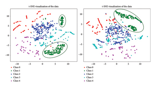
Figure 14 illustrates the adjustments in feature distribution before and after DA using the t-SNE algorithm. The visualization reveals that samples from Class 1 coalesced from two distinct clusters into a single, more cohesive cluster, thereby enhancing the differentiation from other classes and subsequently improving classification efficiency. The DA method operates by mapping the features of test samples to the class prototype features derived from the training set, thereby aligning the feature distribution of the test set to more closely resemble that of the training set.
5.2.5. Analysis of Parameter Sensitivity
In the MF strategy proposed in Section 3, distinct weights are assigned to the different branches constituting the total loss, as illustrated in (7). Specifically, α represents the weight of CL loss, β signifies the weight of classification loss based on contrastive feature representations, γ denotes the weight of classification loss derived from EG features, and δ indicates the weight of classification loss derived from GLCM features. This section investigates the impact of weight parameter combinations on the classification performance of few-shot malware using the MaleVis dataset.
As shown in Table 5, the first parameter set assigns balanced weights across branches as a baseline. Increasing the supervised loss weight β from the first to the second set improves classification performance, with a 0.32% increase in 5-way 1-shot accuracy and a 1.98% increase in 5-way 5-shot accuracy. However, further increasing β to 0.5 reduces accuracy by 0.98% in 5-way 1-shot and 0.31% in 5-way 5-shot scenarios, indicating potential overfitting with excessive supervision weight.
| Setting of weights | 5-way 1-shot | 5-way 5-shot | ||||||
|---|---|---|---|---|---|---|---|---|
| Acc | Pre | Rec | F1 | Acc | Pre | Rec | F1 | |
| α = 0.3, β = 0.3, γ = 0.2, δ = 0.2 | 73.60 | 73.69 | 73.60 | 73.65 | 85.45 | 85.57 | 85.45 | 85.51 |
| α = 0.2, β = 0.4, γ = 0.2, δ = 0.2 | 73.92 | 73.98 | 73.92 | 73.95 | 87.43 | 87.48 | 87.43 | 87.46 |
| α = 0.3, β = 0.5, γ = 0.1, δ = 0.1 | 72.94 | 73.03 | 72.94 | 72.98 | 87.12 | 87.18 | 87.12 | 87.15 |
| α = 0.3, β = 0.4, γ = 0.2, δ = 0.1 | 74.11 | 74.27 | 74.11 | 74.19 | 85.73 | 85.80 | 85.73 | 85.76 |
Experiments show that setting the supervised loss weight β to 0.4 improves classification performance in both 5-way 1-shot and 5-way 5-shot configurations. It is inferred that the combination of contrast learning and multifeature extraction can solve the overfitting problem. In addition, the study finds that among the three features, CL contributes most to model accuracy, followed by EG features and GLCM features. Fine-tuning the weights (fixing supervised loss β at 0.4, increasing CL loss by 0.1, and reducing GLCM loss by 0.1) significantly enhances accuracy in the 5-way 1-shot scenario. Above all, this paper sets the final branch loss weights as α = 0.2, β = 0.4, γ = 0.2, and δ = 0.2, which yield favorable classification performance in both the 5-way 1-shot and 5-way 5-shot configurations.
6. Discussion
To better understand the contributions of each module, we conducted a comprehensive ablation study, with the results presented in Table 6. Here, “w/o” indicates the module that has been removed for analysis.
| Setting of ablation | MaleVis dataset | BIG-2015 dataset | ||||||||||||||
|---|---|---|---|---|---|---|---|---|---|---|---|---|---|---|---|---|
| 5-way 1-shot | 5-way 5-shot | 5-way 1-shot | 5-way 5-shot | |||||||||||||
| Acc | Pre | Rec | F1 | Acc | Pre | Rec | F1 | Acc | Pre | Rec | F1 | Acc | Pre | Rec | F1 | |
| w/o CL&MF&DF | 69.55 | 69.71 | 69.55 | 69.63 | 83.09 | 83.19 | 83.09 | 83.14 | 56.43 | 53.73 | 56.43 | 54.68 | 67.53 | 69.79 | 67.53 | 68.61 |
| w/o MF&DF | 72.66 | 72.79 | 72.66 | 72.72 | 84.38 | 84.47 | 84.38 | 84.43 | 60.77 | 61.04 | 60.77 | 60.91 | 70.61 | 70.65 | 70.61 | 70.63 |
| w/o DF | 74.43 | 74.56 | 74.43 | 74.49 | 87.07 | 87.12 | 87.07 | 87.09 | 65.63 | 65.73 | 65.63 | 65.68 | 73.83 | 73.96 | 73.83 | 73.90 |
| MalFSLDF | 74.26 | 74.32 | 74.26 | 74.29 | 87.56 | 87.48 | 87.56 | 87.52 | 64.33 | 64.57 | 64.33 | 64.45 | 73.92 | 73.97 | 73.92 | 73.94 |
In terms of individual module contributions, the CL module significantly enhanced the model’s performance in scenarios with very few labeled samples, proving to be particularly effective in fine-grained feature learning at the family level. By analyzing the similarities and differences between samples, CL helps the model capture more discriminative texture features. In addition, training the model on multiple backbones forces it to overcome biases between perspectives, further improving the transferability of the learned features.
The MF module demonstrated its strength when applied to larger datasets, leading to a substantial improvement in accuracy. This illustrates the robustness of the MF module in enhancing model performance under different few-shot conditions.
In addition, the DA module showed only a modest improvement in both datasets, suggesting that DA provides incremental benefits in scenarios where the model is already performing well. Despite this, the DA module is still valuable, as it helps normalize feature distributions across distinct malware families and categories, improving the model’s adaptability in few-shot settings.
In summary, the CL module is the most impactful component, enhancing the model’s ability to identify malware families by deeply exploring feature representations. The MF strategy complements this by improving robustness against obfuscated or unknown samples. At the same time, the DA module offers incremental improvements, particularly in scenarios with significant feature domain discrepancies across malware families.
7. Conclusion and Future Work
This paper presents MalFSLDF for the classification of few-shot malware families. This model optimizes feature extraction through a CL strategy and enhances its ability to recognize the characteristics of malware families by adopting MF technology. In addition, the model can adapt to the feature distribution of new types of malware through a DA feature distribution adjustment strategy, further enhancing its generalization capability. Experiments have verified the superior performance of MalFSLDF in the field of malware classification.
Future work can be pursued from two perspectives: on the one hand, more auxiliary features can be explored from the perspective of feature engineering to achieve a more comprehensive representation of malware samples; on the other hand, more advanced domain adaptation methods can be investigated to improve the model’s generalization ability further.
Conflicts of Interest
The authors declare no conflicts of interest.
Funding
This work was supported by the National Natural Science Foundation of China (Grant no. 62172042) and the CCF-NSFOCUS “Kunpeng” Research Fund (Grant no. CCF-NSFOCUS 2023002).
Acknowledgments
This work was supported by the National Natural Science Foundation of China (Grant no. 62172042) and the CCF-NSFOCUS “Kunpeng” Research Fund (Grant no. CCF-NSFOCUS 2023002).
Open Research
Data Availability Statement
Data are available upon request from the corresponding author.


