Neuron Segmentation via a Frequency and Spatial Domain–Integrated Encoder–Decoder Network
Abstract
Three-dimensional (3D) segmentation of neurons is a crucial step in the digital reconstruction of neurons and serves as an important foundation for brain science research. In neuron segmentation, the U-Net and its variants have showed promising results. However, due to their primary focus on learning spatial domain features, these methods overlook the abundant global information in the frequency domain. Furthermore, issues such as insufficient processing of contextual features by skip connections and redundant features resulting from simple channel concatenation in the decoder lead to limitations in accurately segmenting neuronal fiber structures. To address these problems, we propose an encoder–decoder segmentation network integrating frequency domain and spatial domain to enhance neuron reconstruction. To simplify the segmentation task, we first divide the neuron images into neuronal cubes. Then, we design 3D FregSNet, which leverages both frequency and spatial domain features to segment the target neurons within these cubes. Then, we introduce a multiscale attention fusion module (MAFM) that utilizes spatial and channel position information to enhance contextual feature representation. In addition, a feature selection module (FSM) is incorporated to adaptively select discriminative features from both the encoder and decoder, increasing the weight on critical neuron locations and significantly improving segmentation performance. Finally, the segmented nerve fiber cubes were assembled into complete neurons and digitally reconstructed using available neuron tracking algorithms. In experiments, we evaluated 3D FregSNet on two challenging 3D neuron image datasets (the BigNeuron dataset and the CWMBS dataset). Compared to other advanced segmentation methods, 3D FregSNet demonstrates more accurate extraction of target neurons in noisy and weakly visible neuronal fiber images, effectively improving the performance of 3D neuron segmentation and reconstruction.
1. Introduction
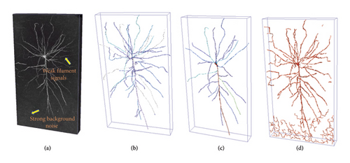
Neuronal morphology plays a significant role in the field of neuroscience. 3D digital reconstruction of neurons aims to establish tree-like models of 3D neuronal morphology using optical microscopy images, which is crucial for understanding the mechanisms of the nervous system and the functions of the brain [1]. However, due to the limitations of current imaging technologies, the quality of the generated 3D brain neuron images varies significantly. As shown in Figure 1, intense background noise and weak neuron signals pose significant challenges to the existing automatic or semiautomatic brain neuron reconstruction algorithms [2–7], making it difficult to achieve accurate neuron reconstruction results. Neuron segmentation, as a preprocessing step, can effectively and automatically denoise and enhance weak signals, making the entire tracking process easier and more precise. In the early stages, some traditional neuron segmentation algorithms were adopted, such as threshold segmentation [8], maximum likelihood global trees [9], 3D tubular models [10], and data-driven methods that encode context-tagged information [11]. However, these methods often require parameter tuning and generally only work well for images with high contrast and clear backgrounds, rendering them a challenge to apply to intricate neuron images. In recent years, deep learning–based methods have gained significant traction in the field of neuron image segmentation. Among them, convolutional neural networks (CNNs) are particularly representative, with 3D U-Net [12] and its variants [13–15] being the most notable examples. However, these advanced algorithms still struggle to precisely extract neuron information from challenging images. First, current deep learning methods typically only extract semantic features in the spatial domain, exhibiting limitations in learning global contextual information. Frequency domain features encapsulate crucial global information about the image. Combining these frequency domain features with spatial domain characteristics can yield a richer, more comprehensive feature representation, thereby enhancing the accuracy of neuron segmentation. Then, by introducing skip connections, the U-Net network can effectively merge low-level and high-level image features. However, this native approach and the constraints of the receptive field can easily result in insufficient processing of multiscale contextual features. Furthermore, at the end of the skip connections, where the feature maps of the decoder and the symmetrical encoder are concatenated and combined, using simple channel concatenation for feature fusion can lead to issues such as feature redundancy and excessive computational overhead.
- 1.
We proposed a neuron segmentation method based on an encoder–decoder network that utilizes both frequency and spatial domains, effectively combining frequency and spatial information for the segmentation of large-scale neuronal images.
- 2.
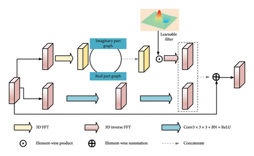
We proposed the FSRA, which performs feature learning in both the frequency and spatial domains, preserving the ability to learn global information while maintaining the integrity of local information.
- 3.
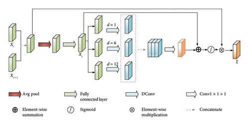
We proposed the MAFM and FSM. The former enhances contextual feature representation by utilizing spatial and channel position information, while the latter adaptively selects features that significantly increase the weight of key neuronal voxels to avoid feature redundancy.
- 4.
Extensive experiments on two 3D neuronal datasets demonstrated that our segmentation results achieve state-of-the-art performance across five different neuron reconstruction algorithms, striking a balance between computational cost and reconstruction performance.
2. Related Works
2.1. 3D Neuronal Reconstruction
Neuronal morphology reconstruction, also known as neuronal tracing, aims to extract quantitative data on neuronal morphology from 3D microscopic images of neurons and establish a 3D morphological structure model of neurons. This process involves identifying all nodes of neural fibers, establishing the topological structure between these points, and measuring the radius information of all nodes. In recent years, numerous experts and scholars in neuron-related fields have developed various automatic or semiautomatic neuronal tracing techniques. For instance, Peng et al. developed APP [16] and APP2 [2], Zhou et al. introduced TReMAP [17], Chen et al. presented SmartTracing [18], Zhao et al. proposed Tube Models [19], Ming et al. developed MOST [3], and the BigNeuron project [20] compiled dozens of tracing algorithms and integrated them into the Vaa3D software [21]. In general, these algorithms leverage graph theory principles to mathematical model neuronal morphology and neural fibers. However, they face two major challenges in practical applications: firstly, they may erroneously identify background noise as neural fibers; secondly, they may overlook a significant number of genuinely existing neural fibers, as illustrated in Figure 1. Despite these tracing algorithms’ high sensitivity to image quality, they often confront a low signal-to-noise ratio due to limitations in current neuronal imaging technologies. Therefore, there is an urgent need for an automatic and rapid algorithm that can reduce noise influence, enhance weak neuronal structures, and ultimately improve the performance of neuronal reconstruction.
2.2. Deep Learning–Based Neuron Segmentation Methods
Before performing neuron reconstruction, implementing accurate neuron segmentation is an effective strategy to enhance the performance of neuron tracing algorithms. In recent years, deep learning–based methods have demonstrated superior performance in medical image analysis without the need for manual feature extraction. Deep learning has also been introduced into neuron image segmentation. For example, Liu et al. [22] proposed a novel 2.5D framework that utilizes a stack of adjacent 2D slices in a 3D image as the input to train a 2D CNN, effectively mitigating substantial background noise in neuron images. Nevertheless, this approach does not take full advantage of the depth information in the 3D image due to the use of 2D convolutions, potentially leading to inaccurate segmentation results. Li et al. [23] introduced the first 3D residual deep network for neuron segmentation to improve 3D neuron reconstruction performance. Liu et al. [13] further enhanced the neuron structure and removed image noise by improving upon the V-Net architecture. Nevertheless, due to the significant imbalance between foreground and background classes in neuron images, this network fails to effectively capture foreground features. To mitigate the aliasing effects caused by downsampling, Li and Shen [14] designed a 3D wavelet integration network to remove data noise. However, suppressing high-frequency information at each downsampling stage leads to excessive loss of edge details. The anisotropy of neuron images results in incomplete preservation of spatial information, causing the loss of some fine neuronal structures. To address this issue, Yang et al. [24] first proposed a two-stage 3D neuron segmentation method. In the first stage, a FCN is trained to obtain a neuron image segmentation map, which is then used to repair broken structures using a Hessian-repair model based on the segmentation results. However, this repair method is complex and time-consuming, and it cannot effectively repair line segments that are too far apart. To achieve clear edge segmentation in vessel images, Xia et al. [25] enhanced the weights of edge voxels through the reverse edge attention block and edge optimization loss. Liu et al. [26] proposed a novel adaptive learning network that utilizes classification results to guide neuron segmentation, reducing model computational complexity and enabling real-time segmentation. However, the advantages of this method often come at the cost of sacrificing some model accuracy. Furthermore, existing neuron segmentation algorithms primarily focus on acquiring spatial domain information while neglecting the importance of frequency domain information. In general computer vision applications, it has been demonstrated that extracting features in the frequency domain is a powerful approach [27, 28]. For instance, GFNet utilizes 2D discrete Fourier transform to replace the self-attention mechanism in ViT [29], employing global filtering layers in the frequency domain to facilitate information exchange between tokens, thereby more effectively capturing long-range dependencies. However, the frequency domain remains underexplored in 3D semantic segmentation. In the spatial domain, the boundaries between segmentation objects and backgrounds are often blurred, whereas in the frequency domain, objects located at different frequencies can be easily distinguished. Inspired by this, we attempted to leverage frequency domain information to improve the performance of 3D neuron image segmentation tasks.
To provide a concise and to-the-point overview, Table 1 lists the usage methods of related work in a tabular form. This table emphasizes the advantages and disadvantages of each method compared to our current method and indicates whether the method belongs to the frequency domain or spatial domain.
| References | Methodology used | Advantages | Disadvantages | Frequency or spatial domain |
|---|---|---|---|---|
| [22] | 2.5D CNN | Easy to train and low computational complexity | Ignoring 3D spatial information | Spatial domain |
| [23] | 3D CNNs | The first 3D residual deep network for neuron segmentation | Inability to effectively segment complex neuron images | Spatial domain |
| [13] | The improved V-Net | Using anisotropic convolutional kernels and varying the number of layers to adapt to neuronal datasets | The network is unable to capture foreground features efficiently | Spatial domain |
| [14] | 3D WaveUNet | The first 3D wavelet integrated network | Suppressing high-frequency information causes the network to excessively lose edge details | Spatial domain |
| [24] | FCN, a ray-shooting model and a Hessian-repair model | Effectively applied to challenging datasets contaminated by noise or containing weak filament signals | The repair method is complicated, time-consuming, and difficult to apply to line segments with excessively large distances. | Spatial domain |
| [25] | ER-Net | Being able to effectively extract spatial edge information | The overall performance is not high, and the computational load is heavy | Spatial domain |
| [26] | ADTL-Net | Short inference time | Sacrificing model accuracy | Spatial domain |
| [27] | Detecting camouflaged object in frequency domain | Introducing frequency domain perception cues into CNN models | Frequency domain unexplored in 3D | Frequency domain |
| [28] | GFNet | 2D DFT replaces the self-attention mechanism, which is simple and computationally efficient | Frequency domain | |
| [30] | SwinUNETR | Excellent global information capture capability | High computational complexity | Spatial domain |
| [31] | 3D UX-Net | Large volumetric convolutional kernel enhances capture of spatial information | High computational resource requirements and relative complexity of the training process | Spatial domain |
3. Methods
3.1. The Method Pipeline
In this study, we developed a pipeline of our 3D neuron segmentation method, as detailed in Figure 2. This method comprises four crucial steps. Specifically, A is partition, where we cut the neuron image into a number of small cubes. The long nerve fibers of neurons may be widely dispersed over larger brain regions, which results in high computational cost when performing 3D neuron segmentation in large-scale images. To reduce this complexity, we adopted a strategy to simplify the segmentation process by cutting the neuron image into a number of small cubes. The dimensions of these cubes were set to be 32 for depth (z-axis), 128 for height (y-axis), and 128 for width (x-axis). B is segmentation, where we use a trained segmentation method to segment the neuronal cubes. C is assembling, where we integrate the segmented neural fibers based on their spatial positions within the neuron image, ultimately achieving the task of 3D neuron segmentation. D is reconstruction, where we utilize the segmented neuron images as a foundation and apply five available tracing algorithms for neuron reconstruction.

3.2. Overall Structure
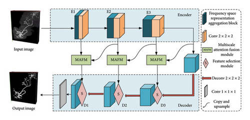
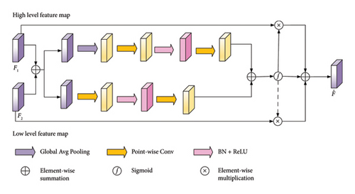
The overall architecture of the proposed segmentation method is shown in Figure 3. This network employs a symmetrical encoder–decoder framework. In the encoder stage, the first three layers consist of a frequency-spatial representation aggregation block followed by a standard convolution with a kernel size of 2 and a stride of 2. After each encoder layer, the feature dimension doubles, while the resolution halves. The skip connections utilized a MAFM to perform cross-scale spatial-channel feature learning, transferring rich contextual information to the decoder. The decoder comprises three layers, each consisting of a FSM and a residual block [32]. Subsequently, a deconvolution with a kernel size of 2 and a stride of 2 is applied for upsampling. Contrary to the encoder, the channel dimension of the feature maps halves after each decoder layer, while the resolution of the feature maps doubles.
3.3. Frequency Space Representation Aggregation Block
3.4. MAFM
3.5. FSM
3.6. Loss Function
The weights of the two loss functions can be controlled by adjusting the value of α in order to achieve the best prediction results.
4. Experiment and Result
4.1. Datasets
- 1.
BigNeuron Dataset: To assess the performance of the presented model, we utilize the gold-166 dataset obtained from the BigNeuron project [20], which encompasses a variety of species such as fish, humans, and mice. The dimensions of the image stacks exhibit variability, such as 2047 × 890 × 23, 724 × 1024 × 33, and 1018 × 543 × 29. To validate the proficiency of our proposed model, we selected 68 neuron images of different types, randomly using 3/4 of them for training and 1/4 for testing.
- 2.
Complex Whole Mouse Brain Sub-Image (CWMBS): In contrast to the BigNeuron dataset, the CWMBS [25] dataset poses a greater challenge due to the notable variations in voxel characteristics across each image. Comprising 83 images with complex background noise and 162 images featuring intricate filamentous structures, all adhering to the dimensions of 256 × 256 × 256 voxels and a spatial resolution of 0.2 × 0.2 × 1.0 μm/voxel. These images are derived from a complete mouse brain and are professionally labeled. We selected 20 images with cluttered background noise and 20 images with fine fibrous structures as the test set, while the rest are used as the training set.
- 3.
Data Labeling: When training deep learning segmentation networks, a large amount of accurate data labels can provide correct guidance to the network. Since the brain neuron dataset used provides expert manually reconstructed results corresponding to each neuron image, where each set of data in the SWC file contains five attributes of the neuron, namely, index, type, location (x, y, and z coordinates), radius, and parent node index [35]. Therefore, one can use Euclidean distance transform (EDT) and these neuron information to automatically generate segmentation labels for each neuron image. The value of each voxel in EDT represents the shortest geometric distance to the target point set, which is defined as shown in the following equation.
() -
where (x1, y1, z1) denotes the 3D coordinates of a voxel in the neuron image, C denotes the set of target points formed by the points on the neuron centerline, and (x2, y2, z2) denotes the 3D coordinates of the voxels in that set. The Euclidean distance is defined as shown in the following equation.
()
4.2. Implementation Details
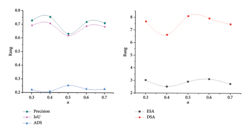
In the experiment, due to significant differences in image size, resolution, signal-to-noise ratio, and neuron morphology between the two datasets, they were trained and tested separately. Furthermore, owing to limitations in computational resources and variations in image dimensions, during the training phase, neuron images were cropped into nonoverlapping 128 × 128 × 32 blocks. Data augmentation was achieved through methods such as random flipping in the X–Y plane, random translation, and noise addition. In the testing phase, the entire test image of arbitrary size was used as input. The model was implemented on an Intel Core CPU and the Pytorch framework with a 24-GB Nvidia RTX 3090 GPU. During training, the SGD optimizer was used for network optimization, with an initial learning rate of 0.1, a weight decay of 0.0005, and a training cycle of 50 epochs. To alleviate the issue of sample imbalance in 3D neuron images, we employed a weighted combination of BCE and Dice loss. To investigate the impact of different α values on the training network, we set different α values on the BigNeuron dataset for network training and testing and used APP2 to reconstruct neurons from segmented images. Then, we evaluated the network’s performance by calculating segmentation metrics such as Precision and IoU, as well as neuron reconstruction metrics including ESA, DSA, and ADS. As shown in Figure 7, when α = 0.4, the network achieved the best overall performance and the most accurate prediction results. Therefore, in subsequent experiments, we set α value to 0.4.
4.3. Evaluation Metrics
Meanwhile, we employed three distance scores to evaluate the discrepancy between the generated reconstruction and the reference reconstruction, namely, the entire structure average (ESA), the different structure average (DSA), and the percentage of different structures (ADS), which are defined in [36]. Specifically, they are calculated in the following ways. For each node in the manual reconstruction, we computed the minimum spatial distance between that node and all nodes in the reconstruction generated by the computational method. The ESA is obtained by averaging all these reciprocal minimum spatial distances across the entire structure. Since it is difficult to visually distinguish nodes separated by less than 2 voxels, the DSA is derived by summing the node pairs with distances greater than 2 voxels between the generated and manual reconstructions of neurons and computing the average. The ADS is obtained by calculating the proportion of node pairs with reciprocal minimum spatial distances greater than 2 voxels among all node pairs. These three evaluation metrics reflect the correctness of neuronal node connections, and the specific values can be generated by the Vaa3D software plugin [21], which directly provides three distance information (ESA, DSA, and ADS) by comparing the computed neuronal reconstruction results (generated SWC file) with the standard manual reconstruction results (standard SWC file). Lower values indicate smaller discrepancies between the generated neuronal reconstruction results and the standard manual reconstruction results, suggesting better neuronal reconstruction performance.
4.4. Evaluation on Images From the BigNeuron Dataset
To comprehensively evaluate the effectiveness of our proposed segmentation method in enhancing the performance of reconstruction algorithms, we conducted extensive comparative experiments. In these comparisons, our method was not only benchmarked against a series of advanced neuronal segmentation methods, including 3D U-Net (M1) [12], 3D Wave-Net (M2) [14], ER-Net (M3) [24], and ADTL-Net (M4) [25] but also against SwinUNETR (M5) [30] and 3D UX-Net (M7) [31], which are currently performing exceptionally well in the field of 3D image processing based on transformer architecture. These comprehensive comparative experiments aimed to validate the effectiveness and superiority of the segmentation model.
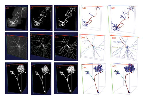
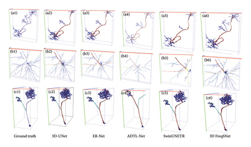
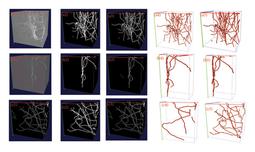
Table 2 shows the segmentation performance of different segmentation methods. It is directly evident from the segmentation test results that 3D FreqSNet outperforms the compared segmentation methods on most metrics. Furthermore, after segmenting the neurons within the cubes, we assemble the cubes into a complete 3D neuronal image. Subsequently, we employed the APP2 algorithm to reconstruct the assembled neurons, thereby generating automatically reconstructed SWC files. Then, we calculated the differences between these automatically reconstructed SWC files and manually reconstructed ones using the Vaa3D software plugin [21], obtaining ESA, DSA, and PDS values to assess the accuracy of the automatic reconstruction. Table 3 shows the three average metrics for 17 test neurons reconstructed using the APP2 algorithm on the segmentation results of different segmentation methods. It can be observed that 3D FreqSNet achieves the best results on the reconstruction metrics ESA and ADS. Although 3D UX-Net obtains relatively good results in PDS, it falls far behind the proposed method in ESA and ADS metrics. This is because 3D UX-Net generates erroneous segmentations due to its self-attention mechanism’s excessive focus on noise. Figure 8 intuitively demonstrates the advantages of 3D FreqSNet. Figures 8(a1) and 8(b1) show neurons with strong background noise, and it can be seen in Figures 8(a2) and 8(b2) that 3D FreqSNet effectively removes the noise. Figures 8(b1) and 8(c1) are neurons with weak filament signals, and it can be seen in Figure 8(b2) and 8(c2) that 3D FreqSNet effectively enhances the weak neuronal signals. 3D FreqSNet significantly improves the segmentation quality of BigNeuron images and enhances neuron reconstruction results. Figure 9 visualizes the reconstruction results generated by various segmentation methods and the ground truth reconstruction. 3D FreqSNet obtains the most accurate and complete reconstruction results among all compared methods, while other methods struggle to obtain precise reconstruction effects, often missing fine neuronal fiber structures (a5 and c4 in Figure 9). The reconstruction results of three complex neuronal images are basically consistent with the ground truth, demonstrating the robustness and versatility of the proposed method.
| Models | Categories | Test results | ||
|---|---|---|---|---|
| Recall↑ | Precision↑ | IoU↑ | ||
| 3D U-Net | Background | 0.9952 | 0.9988 | 0.9941 |
| Target neuron | 0.7611 | 0.4329 | 0.3812 | |
| 3D Wave-Net | Background | 0.9959 | 0.9986 | 0.9946 |
| Target neuron | 0.7176 | 0.4585 | 0.3884 | |
| ADTL-Net | Background | 0.9849 | 0.9997 | 0.9846 |
| Target neuron | 0.9425 | 0.2281 | 0.2250 | |
| ER-Net | Background | 0.9949 | 0.9986 | 0.9935 |
| Target neuron | 0.7178 | 0.4001 | 0.3457 | |
| SwinUNETR | Background | 0.9964 | 0.9984 | 0.9949 |
| Target neuron | 0.6825 | 0.4731 | 0.3878 | |
| 3D UX-Net | Background | 0.9918 | 0.9992 | 0.9911 |
| Target neuron | 0.8373 | 0.3270 | 0.3075 | |
| Ours | Background | 0.9968 | 0.9985 | 0.9954 |
| Target neuron | 0.6981 | 0.5118 | 0.4190 | |
- Note: The bold values represent the best results for the target neuron and background, respectively.
- ↑ indicates that the larger the results of Recall, Precision, and IoU, the better.
| Models | ESA↓ | DSA↓ | ADS↓ |
|---|---|---|---|
| 3D U-Net | 4.9546 | 10.1750 | 0.2584 |
| 3D Wave-Net | 9.0442 | 15.6249 | 0.3361 |
| ADTL-Net | 8.3560 | 14.5661 | 0.3393 |
| ER-Net | 6.6785 | 11.8864 | 0.2735 |
| 3D UX-Net | 4.3721 | 5.9841 | 0.6759 |
| SwinUNETR | 15.9690 | 21.3220 | 0.3538 |
| Ours | 2.4356 | 6.9410 | 0.2120 |
- Note: The bold values indicate that this method performs the best among all methods in each column.
- ↓ indicates that the smaller the results of ESA, DSA, and ADS, the better the performance of this method.
4.5. Evaluation on Images From the CWMBS Dataset
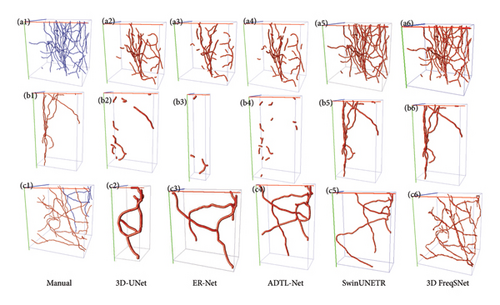
To demonstrate the advantages of the proposed method in processing more challenging images of different categories, we conducted additional experiments using the CWMBS dataset. In this experiment, two groups of images with significant feature differences, namely, strong noise images and weak signal images, were selected to test and validate our method. As shown in Table 4, compared with six other state-of-the-art segmentation methods, the proposed method achieved the best performance in terms of recall, precision, and IoU. The qualitative visualization results of neuron segmentation are shown in Figure 10. By comparing (a1) with (a2) and (b1) with (b2), it is clear that 3D FreqSNet effectively removes noise and enhances the faint filament structures. We also visualized the reconstruction results using the APP2 method on both the original and segmented images, and it is evident that our method makes reconstruction easier and more accurate.
| Models | Categories | Test results | ||
|---|---|---|---|---|
| Recall↑ | Precision↑ | IoU↑ | ||
| 3D U-Net | Background | 0.9990 | 0.9992 | 0.9982 |
| Target neuron | 0.2342 | 0.1904 | 0.1173 | |
| 3D Wave-Net | Background | 0.9996 | 0.9991 | 0.9989 |
| Target neuron | 0.1185 | 0.3355 | 0.0957 | |
| ADTL-Net | Background | 0.9992 | 0.9992 | 0.9984 |
| Target neuron | 0.2319 | 0.2321 | 0.1312 | |
| ER-Net | Background | 0.9981 | 0.9997 | 0.9979 |
| Target neuron | 0.7879 | 0.2945 | 0.2728 | |
| SwinUNETR | Background | 0.9994 | 0.9995 | 0.9989 |
| Target neuron | 0.4936 | 0.4730 | 0.3185 | |
| 3D UX-Net | Background | 0.9993 | 0.9995 | 0.9989 |
| Target neuron | 0.5548 | 0.4506 | 0.3309 | |
| Ours | Background | 0.9993 | 0.9996 | 0.9989 |
| Target neuron | 0.5985 | 0.4747 | 0.3601 | |
- Note: Each column in bold represents the best results for the target neuron and background, respectively.
- ↑ indicates that the larger the results of Recall, Precision, and IoU, the better.
The comparison of reconstruction results using different segmentation methods is shown in Figure 11. Previous state-of-the-art methods such as 3D U-Net, ER-Net, and ADTL-Net produce discontinuous segmentations, leading to incomplete reconstructed structures (b2, b3, and b4 in Figure 11). SwinUNETR oversegments noisy images, resulting in unnecessary scatter (b5 in Figure 11). In contrast, 3D FreqSNet achieves better reconstruction results, further demonstrating that our method greatly benefits noise reduction and enhancement of neuron structure signals.
4.6. Comparison of Different Reconstruction Algorithms
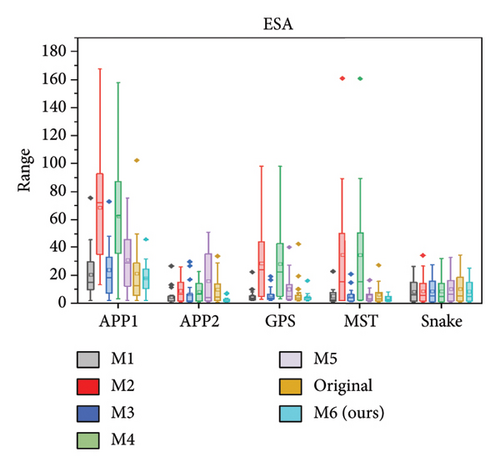
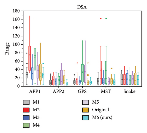
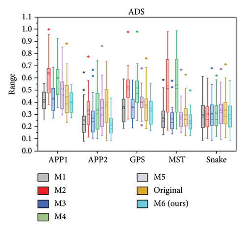
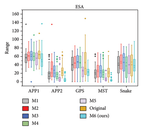
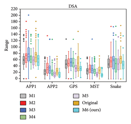
We further quantitatively evaluated the impact of 3D FreqSNet on different neuron reconstruction algorithms. Comparisons of other segmentation methods were conducted on five available neuron reconstruction algorithms, namely, APP1 [16], APP2 [2], NeuroGPS-Tree (GPS) [37], MST_Tracing (MST) [38], and Snake [39]. The box plot of the quantitative analysis is shown in Figures 12(a), 12(b), and 12(c). Compared with reconstructing neuron structures directly from images without any preprocessing, the segmentation maps generated by the proposed model showed significant improvements in various reconstruction metrics. It can also be observed that after applying the five reconstruction algorithms, 3D FreqSNet outperformed other segmentation methods used for comparison in most neuron reconstruction measurement metrics. Due to the loss of a large number of nerve fibers in the segmentation results of 3D Wave-Net (M2) and ADTL-Net (M4), the reconstruction results were worse than those obtained on the original images. Similarly, as shown in Figures 12(d), 12(e), and 12(f), 3D FreqSNet significantly improved the performance of the five reconstruction algorithms on CWMBS test images, outperforming the reconstruction results on the original images in various quantitative metrics. Compared with the M1–M6 segmentation methods, the reconstruction metrics performed better. Overall, our proposed method can extract more complete neuron structures when processing complex images, which greatly simplifies the subsequent neuron tracing process and further improves the reconstruction performance of the BigNeuron and CWMBS datasets.

4.7. Computational Complexity Analysis
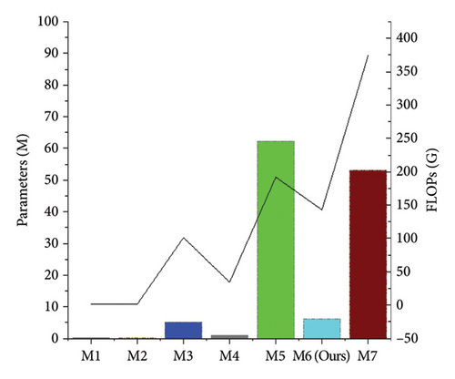
In a clinical setting, computational complexity is an important metric. The number of model parameters and floating point operations per second (FLOPs) are used to evaluate the computational complexity of different methods. The number of parameters in our model is 6.24 M, and the floating-point operations (FLOPs) required are 143.25 G. As shown in Figure 13, SwinUNETR (M5) and 3D UX-Net (M7) have a large number of parameters and high computational costs due to the quadratic complexity of their self-attention mechanisms, which limit their application in large-scale neuronal reconstruction. Methods such as 3D U-Net (M1), 3D Wave-Net (M2), ER-Net (M3), and ADTL-Net (M4) have relatively smaller model parameter counts and floating-point operation counts, but their neuronal reconstruction performance is not high. As can be seen from Figure 13, Tables 3 and 5, our method achieves a better balance between accuracy and computational cost, making it more suitable for clinical experiments and the reconstruction of very large-scale neurons.
| Category | Method | ESA↓ | DSA↓ | ADS↓ |
|---|---|---|---|---|
| Strong noise | 3D U-Net | 15.0077 | 19.8790 | 0.4669 |
| 3D Wave-Net | 24.3382 | 29.0396 | 0.4943 | |
| ER-NET | 22.3417 | 27.1394 | 0.4831 | |
| ADTL-Net | 12.6981 | 17.2158 | 0.4778 | |
| 3D UX-Net | 5.3132 | 13.0049 | 0.2672 | |
| SwinUNETR | 6.8669 | 13.0615 | 0.2987 | |
| Ours | 4.7137 | 12.7418 | 0.2413 | |
| Weak signal | 3D U-Net | 24.7178 | 29.0057 | 0.4561 |
| 3D Wave-Net | 36.7628 | 40.7563 | 0.5590 | |
| ER-NET | 32.2134 | 41.8694 | 0.4647 | |
| ADTL-Net | 23.3912 | 30.7686 | 0.5375 | |
| 3D UX-Net | 9.1634 | 16.6115 | 0.2569 | |
| SwinUNETR | 13.2005 | 19.1474 | 0.3464 | |
| Ours | 6.3835 | 13.0442 | 0.2126 | |
- Note: The bold values indicate that this method performs the best among all methods in each column.
- ↓ indicates that the smaller the results of ESA, DSA, and ADS, the better the performance of this method.
4.8. Ablation Experiments
4.8.1. Ablation Experiments With 3D FreqSNet
In this method, we proposed the FSRA, MFAM, and FSM. To demonstrate the effectiveness of these modules, comprehensive ablation experiments were conducted on both the BigNeuron dataset and the CWMBS dataset. As shown in Table 6, the APP2 reconstruction method was used to measure 17 images in BigNeuron and 40 images in CWMBS, respectively. In addition, we also calculated the average inference time for the BigNeuron test images associated with each variant. Firstly, to verify the effectiveness of the backbone network, we replaced the original blocks in 3D U-Net with ResBlock and denoted it as ResU-Net. By comparing Tables 3 and 6, the results indicated that ResU-Net improved the ESA, DSA, and ADS reconstruction results by 1.1002, 1.3456, and 0.0363, respectively, on the BigNeuron dataset. Furthermore, by comparing Tables 5 and 6, the ESA, DSA, and ADS of 3D U-Net on the CWMBS dataset are 19.8627, 24.4423, and 0.4615, respectively, while those of ResU-Net are 10.1511, 15.9947, and 0.3368, respectively, which further demonstrates the effectiveness of the backbone network. Then, we conducted ablation experiments on the proposed modules based on ResU-Net (Net1).
| Design | Backbone | Modules | Parm (M) | Inference time (S) | BigNeuron | CWMBS | ||||||
|---|---|---|---|---|---|---|---|---|---|---|---|---|
| ResU-Net | FSAB | MFAM | FSM | ESA↓ | DSA↓ | ADS↓ | ESA↓ | DSA↓ | ADS↓ | |||
| Net1 | √ | 7.34 | 7.44 | 3.8554 | 8.8294 | 0.2220 | 10.1511 | 15.9947 | 0.3368 | |||
| Net2 | √ | √ | 6.42 | 7.11 | 3.2351 | 7.8325 | 0.2132 | 8.0932 | 15.7590 | 0.2563 | ||
| Net3 | √ | √ | √ | 5.28 | 11.67 | 2.8864 | 7.5045 | 0.2199 | 7.9587 | 15.4347 | 0.2560 | |
| Net4 | √ | √ | √ | 6.82 | 18.23 | 2.7337 | 7.0147 | 0.2103 | 6.4211 | 14.5223 | 0.2358 | |
| Net5 | √ | √ | √ | √ | 6.24 | 15.23 | 2.5048 | 6.9185 | 0.2095 | 5.5486 | 12.8930 | 0.2269 |
- Note: The bold values indicate that this method performs the best among all methods in each column.
- ↓ indicates that the smaller the results of ESA, DSA, and ADS, the better the performance of this method.
Net2 replaces the ResBlock in Net1 with the FSRA. On the BigNeuron and CWMBS datasets, the neuron reconstruction metrics ESA improved by 0.6203 and 2.0579, respectively, DSA improved by 0.9969 and 0.2357, respectively, and ADS improved by 0.0088 and 0.0805, respectively. Compared to only retaining the spatial domain (Net1), introducing the FFT (Net2) significantly improves performance, indicating that the model can capture richer global information in the frequency domain, which is beneficial for improving neuron structure reconstruction performance. The FSRA module enhances the network’s learning capability by simultaneously learning information from both the spatial and frequency domains, thereby reducing noise interference and better capturing texture shapes.
To demonstrate the effectiveness of the MFAM, after removing the MFAM module from our model, the ESA of the two datasets decreased by 0.3816 and 2.4101, respectively, DSA decreased by 0.586 and 2.5417, respectively, and ADS decreased by 0.0104 and 0.0291, respectively, due to the lack of the ability to utilize cross-layer contextual features.
Similarly, if the FSM is not used, the model’s ability to adaptively select important features will be greatly weakened, which is also clearly reflected in the reconstruction metrics of the two datasets. The ESA decreased by 0.2289 and 1.6293, respectively, DSA decreased by 0.0962 and 1.6293, respectively, and ADS decreased by 0.8725 and 0.0089, respectively. In addition, the model parameters and inference time also increased slightly because the lack of FSM increases redundant feature calculations and reduces inference efficiency.
The outstanding performance of 3D FreqSNet is attributed to the synergistic effect of FSRA, MFAM, and FSM, which together enable the model to effectively capture complex spatial and frequency dependencies and accurately and robustly extract valuable features necessary for neuron image segmentation.
4.8.2. Ablation Experiments on the FSRA Module
To verify the impact of the FFT and spatial domain convolutional branches on the internal performance of FSAB, we conducted ablation experiments on FSAB, as shown in Table 7. Firstly, after removing the FFT and 3 × 3 × 3 convolutional block (replaced with Conv1 × 1 × 1), the ESA, DSA, and ADS of the BigNeuron dataset were 3.3526, 8.6201, and 0.2446, respectively, while those of the CWMBS dataset were 11.6143, 21.0707, and 0.2998, respectively. Compared to retaining the FFT and Conv3 × 3 × 3, performance decreased, indicating that ordinary convolutions are difficult to fully capture global information. Subsequently, compared to the case of not using both FFT and Conv3 × 3 × 3, introducing only spatial domain convolutions did not significantly improve the ESA, DSA, and ADS values. In contrast, introducing only the FFT significantly improved performance, indicating its ability to capture rich global information in the frequency domain. Finally, when both FFT and Conv3 × 3 × 3 were used, the ESA, DSA, and ADS of the BigNeuron dataset were 2.5048, 6.9185, and 0.2095, respectively, while those of the CWMBS dataset were 5.5486, 12.8930, and 0.2269, respectively. This demonstrates that combining FFT and Conv3 × 3 × 3 can effectively utilize the complementary advantages of the frequency and spatial domains, achieving excellent segmentation and reconstruction performance.
| FFT | Spatial branch | BigNeuron | CWMBS | ||||
|---|---|---|---|---|---|---|---|
| ESA | DSA | ADS | ESA | DSA | ADS | ||
| — | — | 3.3526 | 8.6201 | 0.2446 | 11.6143 | 21.0707 | 0.2998 |
| — | √ | 3.9955 | 8.5949 | 0.2420 | 11.8177 | 17.5911 | 0.3517 |
| √ | — | 2.8876 | 7.1483 | 0.2195 | 6.8812 | 13.4469 | 0.2723 |
| √ | √ | 2.5048 | 6.9185 | 0.2095 | 5.5486 | 12.8930 | 0.2269 |
- Note: The bold values indicate that this method performs the best among all methods in each column.
4.8.3. Visualization of Ablation Experiments
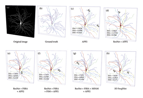
Figure 14 intuitively visualizes the reconstruction of an example neuron image. Figure 14(a) shows the original image, and Figure 14(b) shows the manually reconstructed neuron, which accurately depicts the morphological structure of the neuron. Figure 14(c) displays the neuron reconstruction result of APP2 on the original image, while Figure 14(d) shows the APP2 reconstruction result based on the segmentation map of ResU-Net. The following three images are the APP2 reconstruction results of segmented neuron images under different ablation modules. Figure 14(h) presents the APP2 reconstruction on the neurons segmented by 3D FreqSNet. On the original image, APP2 is not only susceptible to noise interference, overtracking noise as nerve fibers, but also stops tracking weak-signal neurons. By comparing Figures 14(d), 14(e), 14(f), 14(g), and 14(h), it can be observed that after adding FSRA, MFAM, and FSM, respectively, the neuron reconstruction performance improves progressively, further demonstrating the effectiveness of these modules. As indicated by the yellow arrows, 3D FreqSNet captures richer texture details and achieves more complete reconstructions, illustrating its feasibility in suppressing noise and enhancing weak neuronal fiber structures.
5. Conclusion
In this study, we proposed a frequency and spatial domain integrated encoder–decoder 3D segmentation network, called 3D FreqSNet, which mainly consists of three modules: the FSRA, the MAFM, and the FSM. Firstly, the FSRA extracts global and local information from frequency and spatial domain feature maps, effectively integrating frequency spatial information and reducing the network’s susceptibility to noise. Secondly, the MFAM enhances multiscale contextual perception capabilities by integrating and fusing spatial and channel positional information. Finally, the FSM avoids feature redundancy by adaptively selecting features from the encoder and decoder at the same hierarchy level. We conducted extensive experiments on two complex 3D neuron image datasets, and the results show that the proposed model not only significantly improves the reconstruction results of five existing neuron tracing algorithms but also demonstrates clear advantages compared to other advanced neuron segmentation methods in improving neuron reconstruction performance. At the same time, it exhibits higher accuracy in segmenting neuron images with strong background noise and weak voxel signals. In addition, 3D FreqSNet achieves a good balance between accuracy and computational cost, which is more conducive to large-scale neuron reconstruction.
However, this study still has some limitations. Firstly, the threshold α of the proposed loss function needs to be manually adjusted according to the dataset, which requires subjective experience. To address this, we will develop an automatic method to achieve adaptive setting of α in the future. Secondly, the proposed segmentation algorithm is based on fully supervised learning, requiring corresponding manually reconstructed annotation data. However, large-scale manual annotation of neurons demands extensive neurobiology knowledge and human resources, making it difficult to obtain. To reduce the need for a large amount of annotated data, we will explore the use of semisupervised, transfer learning, or active learning methods in the future to achieve more positive results. Finally, this study only explores the reconstruction of neurons on two animal brain slices. In the future, we will further explore the reconstruction of ultra-large–scale neuronal clusters on whole-brain images of animals, which will contribute to the analysis of brain neural networks and brain functional mechanisms, thereby promoting further research on brain cognition, brain diseases, and other aspects.
Conflicts of Interest
The authors declare no conflicts of interest.
Author Contributions
Haixing Song: writing–review and editing, writing–original draft, software, methodology, formal analysis, and conceptualization. Xuqing Zeng: writing–review and editing, visualization, and validation. Guanglian Li: supervision, resources, and formal analysis. Rongqing Wu: methodology and conceptualization. Simin Liu: resources and data curation. Fuyun He: supervision, resources, project administration, and funding acquisition.
Funding
This work was supported by the National Natural Science Foundation of China (No. 62062014) and the grant from Guangxi Key Laboratory of Brain-inspired Computing and Intelligent Chips (No. BCIC-23-Z1).
Open Research
Data Availability Statement
The data that support the findings of this study are available from the corresponding author upon reasonable request.


