International Journal of Intelligent Systems

Volume 2025, Issue 1 5309734

Research Article

Open Access

JPEG Image Steganography With Automatic Embedding Cost Learning

Jianhua Yang

orcid.org/0000-0003-1354-9230

Department of Cyber Security , School of Cyber Security , Guangdong Polytechnic Normal University , Guangzhou , Guangdong, China , gdin.edu.cn

Search for more papers by this author

Yi Liao,

Yi Liao

orcid.org/0009-0007-4577-8501

Department of Computer Science , School of Computer Science and Engineering , South China University of Technology , Guangzhou , Guangdong, China , scut.edu.cn

Search for more papers by this author

Fei Shang,

Fei Shang

orcid.org/0000-0003-4037-259X

Department of Computer Science , Guangdong Key Laboratory of Information Security , Sun Yat-sen University , Guangzhou , Guangdong, China , sysu.edu.cn

Search for more papers by this author

Xiangui Kang,

Xiangui Kang

orcid.org/0000-0002-3134-0353

Department of Computer Science , Guangdong Key Laboratory of Information Security , Sun Yat-sen University , Guangzhou , Guangdong, China , sysu.edu.cn

Search for more papers by this author

Yifang Chen,

Corresponding Author

Yifang Chen

[email protected]

orcid.org/0009-0002-7129-9153

Department of Cyber Security , School of Cyber Security , Guangdong Polytechnic Normal University , Guangzhou , Guangdong, China , gdin.edu.cn

Search for more papers by this author

Yun-Qing Shi,

Yun-Qing Shi

Department of ECE , New Jersey Institute of Technology , Newark , New Jersey, USA , njit.edu

Search for more papers by this author

Jianhua Yang,

Jianhua Yang

orcid.org/0000-0003-1354-9230

Department of Cyber Security , School of Cyber Security , Guangdong Polytechnic Normal University , Guangzhou , Guangdong, China , gdin.edu.cn

Search for more papers by this author

Yi Liao,

Yi Liao

orcid.org/0009-0007-4577-8501

Department of Computer Science , School of Computer Science and Engineering , South China University of Technology , Guangzhou , Guangdong, China , scut.edu.cn

Search for more papers by this author

Fei Shang,

Fei Shang

orcid.org/0000-0003-4037-259X

Department of Computer Science , Guangdong Key Laboratory of Information Security , Sun Yat-sen University , Guangzhou , Guangdong, China , sysu.edu.cn

Search for more papers by this author

Xiangui Kang,

Xiangui Kang

orcid.org/0000-0002-3134-0353

Department of Computer Science , Guangdong Key Laboratory of Information Security , Sun Yat-sen University , Guangzhou , Guangdong, China , sysu.edu.cn

Search for more papers by this author

Yifang Chen,

Corresponding Author

Yifang Chen

[email protected]

orcid.org/0009-0002-7129-9153

Department of Cyber Security , School of Cyber Security , Guangdong Polytechnic Normal University , Guangzhou , Guangdong, China , gdin.edu.cn

Search for more papers by this author

Yun-Qing Shi,

Yun-Qing Shi

Department of ECE , New Jersey Institute of Technology , Newark , New Jersey, USA , njit.edu

Search for more papers by this author

First published: 16 February 2025

https://doi.org/10.1155/int/5309734

Academic Editor: Hongyang Yan

Share a link

Email
Wechat
Bluesky

Abstract

A great challenge to steganography has arisen with the wide application of steganalysis methods based on convolutional neural networks (CNNs). To this end, embedding cost learning frameworks based on generative adversarial networks (GANs) has been proposed and achieved success for spatial image steganography. However, the application of GAN to JPEG steganography is still in the prototype stage; its antidetectability and training efficiency should be improved. In conventional steganography, research has shown that the side information calculated from the precover can be used to enhance security. However, it is hard to calculate the side information without the spatial domain image. In this work, an embedding cost learning framework for JPEG image steganography via a GAN (JS–GAN) has been proposed, the learned embedding cost can be further adjusted asymmetrically according to the estimated side information (ESI). Experimental results have demonstrated that the proposed method can automatically learn a content-adaptive embedding cost function, and using the ESI properly can effectively improve the security performance. For example, under the attack of a classic steganalyzer GFR with a quality factor of 75 and 0.4 bpnzAC, the proposed JS–GAN can increase the detection error by 2.58% over J-UNIWARD, and the ESI–aided version JS–GAN (ESI) can further increase the security performance by 11.25% over JS–GAN.

1. Introduction

JPEG steganography is a technology that aims at covert communication, through modifying the coefficients of the discrete cosine transform (DCT) of an innocuous JPEG image. By restricting the modification to the complex area or the low-frequency area of the DCT coefficients, content-adaptive steganographic schemes guarantee satisfactory antidetection performance, which has become a mainstream research direction. Since the Syndrome-Trellis Codes (STCs) [1] can embed a given payload with a minimal embedding impact, current research on content-adaptive steganography has mainly focused on how to design a reasonable embedding cost function [2–5].

In contrast, steganalysis methods try to detect whether the image has secret messages hidden in it. Conventional steganalysis methods are mainly based on statistical features with ensemble classifiers [6–8]. To further improve the detection performance, the selection channel has been incorporated for feature extraction [9, 10]. In recent years, steganalysis methods based on convolutional neural networks (CNNs) have been researched, initially in the spatial domain [11–14], and have also achieved success in the JPEG domain [15–18]. Current research has shown that a CNN–based steganalyzer can reduce the detection error dramatically compared with conventional steganalyzers, and the security of conventional steganography faces great challenges.

With the development of deep neural networks, recent work has proposed an automatic stegagography method to jointly train the encoder and decoder networks. The encoder can embed the message and generate an indistinguishable stego image. Then, the message can be recovered from the decoder. However, the security may reduced due to the larger capacity [19–22].

In the conventional steganographic scheme, the embedding cost function is designed heuristically, and the measurement of the distortion cannot be adjusted automatically according to the strategy of the steganalysis algorithm. Frameworks for automatically learning the embedding cost by adversarial training have been proposed and can achieve better performance than the conventional method in the spatial domain [23–25]. In [23], the authors proposed an automatic steganographic distortion learning framework with generative adversarial networks (ASDL–GANs), which can generate an embedding cost function for spatial steganography. U-Net and double-tanh function with GAN–based framework (UT–GAN) [24] further enhanced the security performance and training efficiency of the GAN–based steganographic method by incorporating a U-Net [26]-based generator and a double-tanh embedding simulator. The influence of high pass filters in the preprocessing layer of the discriminator was also investigated. Experiments show that UT–GAN can achieve a better performance than the conventional method. Steganographic pixelwise actions and rewards with reinforcement learning (SPAR–RL) [25] uses reinforcement learning to improve the loss function of GAN–based steganography, and experimental results show that it further improves the stable performance. Although embedding cost learning has been developed in the spatial domain, it is still in its initial stages in the JPEG domain. In our previous conference presentation [27], we proposed a JPEG steganography framework based on GAN to learn the embedding cost. Experimental results show that it can learn the adaptivity and achieve a performance comparable to that of the conventional methods. In [23], JPEG domain knowledge has been used to improve the performance.

To preserve the statistical model of the cover image, some steganography methods use the knowledge of the so-called precover [28]. The precover is the original spatial image before JPEG compression. In conventional methods, previous studies have shown that using asymmetric embedding, namely, +1 and −1 processes with different embedding costs, can further improve the security performance. Side-informed (SI) JPEG steganography calculates the rounding error of the DCT coefficients with respect to the compression step of the precover and then uses the rounding error as the SI to adjust the embedding cost for asymmetric embedding [29]. However, it is hard to obtain the SI without the precover, so the researcher tries to estimate the precover to calculate the estimated SI (ESI). In [30], a precover estimation method that uses series filters was proposed. The experimental results show that although it is hard to estimate the amplitude of the rounding error, the security performance can be improved by using the polarity of the estimated rounding error.

Although initial studies of the automatic embedding cost learning framework have shown that it can be content-adaptive, its security performance and training efficiency should be improved. In conventional steganography, the SI estimation is heuristically designed, and the precision of the estimation depends on experience and experiments. How to estimate the SI through CNN and adjust the embedding cost asymmetrically with the unprecise SI needs to be investigated.

In the present paper, we extend [27], and the learned embedding cost can be further adjusted asymmetrically according to the ESI. The main contributions of this paper can be summarized as follows:

1.
We further develop the GAN–based method of generating an embedding cost function for JPEG steganography. Unlike conventional hand-crafted cost functions, the proposed method can automatically learn the embedding cost via adversarial training.
2.
To solve the gradient-vanishing problem of the embedding simulator, we propose a gradient-descent–friendly embedding simulator to generate the modification map with a higher efficiency.
3.
Under the condition of lacking the uncompressed image, we propose a CNN–based SI estimation method. The estimated rounding error has been used as the SI for asymmetrical embedding to further improve the security performance.

The rest of this paper is organized as follows. In Section 2, we briefly introduce the basics of the proposed steganographic algorithm, which includes the concept of distortion minimization framework and SI JPEG steganography. A detailed description of the proposed GAN–based framework and the SI estimation method is given in Section 3. Section 4 presents the experimental setup and verifies the adaptivity of the proposed embedding scheme. The security performance of our proposed steganography under different payloads compared with the conventional methods is also shown in Section 4. Our conclusions and avenues for future research are presented in Section 5.

2. Preliminaries

2.1. Notation

In this article, the capital symbols stand for matrices, and i and j are used to index the elements of the matrices. The symbols C = (C_i,j), S = (S_i,j) ∈ R^h×w represent the 8-bit grayscale cover image and its stego image of size h × w, respectively, where S_i,j ∈ {max(C_i,j − 1, 0), C_i,j, min(C_i,j + 1, 255)}. p = (p_i,j) denotes the embedding probability map. N = (n_i,j) stands for a random matrix with a uniform distribution ranging from 0 to 1. M = (m_i,j) stands for the modification map, where m_i,j ∈ {−1, 0, 1}.

2.2. Distortion Minimization Framework

Most of the successful steganographic methods embed the payload by obeying a distortion minimization rule that the sender embeds a payload of m bits while minimizing the average distortion [1], that is,

()

where π(S) stands for the modification distribution of modifying C to S and D(S) is the distortion function that measures the impact of embedding modifications and is defined as

()

where ρ_i,j represents the cost of replacing the C_i,j with S_i,j . In most symmetric embedding schemes, the costs of increasing or decreasing C_i,j by 1 are equal during embedding, i.e.,

= ρ_i,j . The optimal solution of equation (1) has the form of a Gibbs distribution [31] as follows:

()

where the scalar parameter λ > 0 needs to be calculated from the payload constraint in equation (2)

2.3. SI JPEG Steganography

SI JPEG steganography uses the additional message to adjust the cost for better embedding. In [29], the rounding error of the DCT coefficient is calculated from the precover, and then the embedding cost is adjusted by using the rounding error as the SI for an asymmetric embedding. For a given precover, the rounding error is defined as follows:

()

where U_i,j is the nonrounded DCT coefficient and C_i,j is the rounded DCT coefficient of the cover image. When generating the stego S by using the ternary embedding steganography with SI, the embedding cost ρ_i,j is calculated at first, and then the costs of changing C_i,j by ± sign(e_i,j) can be adjusted as follows:

()

When the precover is unavailable [30], the SI is estimated from the precover by first using series filters, and then calculating the estimated rounding error

to be the SI with which to adjust the embedding cost.

()

where η is used to make sure the embedding cost is positive when the absolute value of the SI is greater than 0.5. It should be noted that steganography with ESI is even inferior to the methods without SI due to the imprecision in the amplitude of the rounding error. To solve this problem, the authors proposed a method using polarity to adjust the embedding cost. The sign of the SI is used to adjust the cost, and the amplitude is ignored.

()

3. The Proposed Cost Function Learning Framework for JPEG Steganography

In this section, we propose an embedding cost-learning framework for JPEG steganography based on GAN (JS–GAN). We conduct an ESI based on CNN to asymmetrically adjust the embedding cost to further improve the security, and the version which uses ESI as a help is referred to as JS–GAN (ESI).

3.1. JS–GAN

The overall architecture of the proposed JS–GAN is shown in Figure 1. The solid line and dashed line denote the forward and backpropagation, respectively. It is mainly composed of four modules: a generator, an embedding simulator, an IDCT module, and a discriminator. The training steps are described in Algorithm 1.

Details are in the caption following the image — **Figure 1**
Open in figure viewer PowerPoint

Architecture of the proposed JS–GAN.

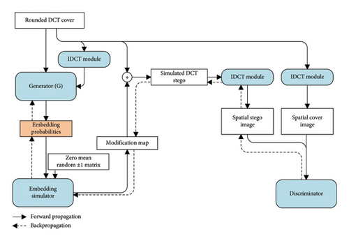
For an input of a rounded DCT matrix C, the p_i, j ∈ [0, 1] denotes the corresponding embedding probability produced by the adversarially trained generator. Since the probabilities of increasing or decreasing C_i,j are equal, we set and the probability that C_i,j remains unchanged is ^. We also feed the spatial cover image converted from the rounded DCT matrix into the generator to improve the performance of our method.

Algorithm 1: Training steps of JS–GAN.

Require:
Rounded DCT matrix of the cover image.
Zero mean random ±1 matrix.
Step 1: Input the rounded DCT matrix of the cover image and the corresponding spatial cover image into the generator to obtain the embedding probability.
Step 2: Generate a modification map using the proposed embedding simulator.
Step 3: Add the modification map into the DCT coefficients’ matrix of the cover image to generate the DCT coefficients’ matrix of the stego image.
Step 4: Convert the cover and stego DCT coefficients’ matrix to the spatial image by using the IDCT module.
Step 5: Feed the spatial cover–stego pair into the discriminator to obtain the loss of the generator and discriminator.
Step 6: Update the parameters of the generator and discriminator alternately, using the gradient descent optimization algorithm of Adam to minimize the loss.

The embedding simulator is used to generate the corresponding modification map. The DCT matrix of the stego image is obtained by adding the modification map to the DCT matrix of the cover image. By applying the IDCT module [27], we can finally produce the spatial cover–stego image pair. The discriminator tries to distinguish the spatial stego images from the innocent cover images. Its classification error is regarded as the loss function to train the discriminator and generator using the gradient descent optimization algorithm.

After training the JS–GAN as shown in Algorithm 1 with 0.5 bit per nonzero AC (bpnzAC) DCT coefficient payload for a certain number of iterations, the trained generator is capable of generating an embedding probability, which is then used for the follow-up steganography. Since the embedding cost should be constrained to 0 ≤ ρ_i,j ≤ ∞, it can be computed based on the embedding probability p_i,j as follows [33]:

()

To further improve the performance, the embedding costs from the same location of DCT blocks have been smoothed by a Gaussian filter as a postprocess [34]. The incorporation of this Gaussian filter will improve the security performance by about 1.5%. After designing the embedding cost, the STC encoder [1] has been applied to embed the specific secret messages to generate the actual stego image. Detailed descriptions of each module of JS–GAN will be given in the following sections.

3.1.1. Architecture of the Generator G

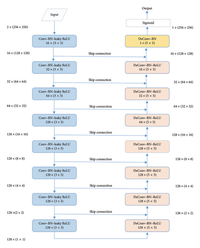
The main purpose of JS–GAN is to train a generator that can generate the embedding probability with the same size as the DCT matrix of the cover image, and the process step can be regarded as an image-to-image translation task. Based on the superior performance in image-to-image translation and high training efficiency, we use U-Net [26] as a reference structure to design our generator. The generator of JS–GAN contains a contracting path and an expansive path with 16 groups of layers. The contracting path is composed of eight operating groups: each group includes a convolutional (Conv) layer with Stride 2 for downsampling, a batch normalization (BN) layer, and a leaky rectified linear unit (Leaky-ReLU) activation function. The expansive path consists of the repeated application of the deconvolution layer, each time followed by a BN layer and ReLU activation function. After upsampling the feature map to the same size as the input, the final sigmoid activation function is added to restrict the output within the range of 0–1 in order to meet the requirements of being an embedding probability. To achieve pixel-level learning and facilitate the backpropagation, concatenations of feature maps are placed between each pair of mirrored Conv and deconvolution layers by using a skip connection process. The specific configuration of the generator is given in Figure 2.

3.1.2. The Embedding Simulator

As shown in Figure 1, an embedding simulator is required to generate the corresponding modification map according to the embedding probability. Conventional steganography methods [2, 33, 35–37] use a staircase function [38] to simulate the embedding process as follows:

()

where m_i,j is the modification map with values ±1 and 0, n_i,j stands for a random number from the uniform distribution on the interval [0, 1], and p_i,j is the embedding probability.

Although equation (11) has been widely used in conventional methods, the staircase function cannot be put into the pipeline of the training phase of GAN because most of the derivatives are zero, which will lead to the gradient-vanishing problem. In the present paper, we propose an embedding simulator that uses the learned embedding probability. Since the primary target of the embedding simulator in JS–GAN is to make more modifications of the elements with a higher embedding probability, we use the probability as a modification map. The stego DCT matrix is generated by adding the cover DCT matrix and the corresponding modification map. It should also be noticed that the learned probabilities range from 0 to 1, which cannot simulate a modification with a negative sign. To solve this problem, our proposed embedding simulator multiplies the embedding probability map with a zero mean random ±1 matrix to obtain the modification map m_i,j. The specific implementation of our proposed embedding simulator is given in the following equation:

()

where [p] is the Iverson bracket, i.e., equal to 1 when the statement p is true and 0 otherwise. The embedding simulator we proposed can generate the corresponding DCT matrix of stego efficiently and is gradient-descent–friendly. Experimental results also prove that applying this embedding simulator in our JS–GAN means it can learn an adaptive embedding probability.

3.1.3. Architecture of the Discriminator D

In [17], we used a DenseNet-based steganalyzer as the discriminator. Since the feature concatenation consumes more GPU memory and training time than the add process, we used a refined residual network–based J-XuNet [16] as the discriminator. The details of the discriminator are shown in Figure 3. Against the Gabor filter–based discriminator, a preprocessing layer that incorporates 16 Gabor high-pass filters is used to implement a Conv operation to the input image. Gabor high-pass filters can effectively enhance the steganographic signal and help subsequent neural networks extract steganographic features better. The Gabor filters are defined as follows:

()

where μ = xcosθ + ysinθ and v = xsinθ + ycosθ. σ is the standard deviation of the Gaussian factor and λ is the wavelength, σ = 0.56λ meanwhile σ = (0.75, 1). Directional coefficient θ = (0, π/4, 2π/4, 3π/4), phase offset ϕ = (0, π/2), and aspect ratio γ = 0.5.

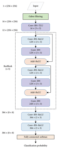
After the preprocessing layer, a Conv block that consists of a truncated linear unit (TLU) [39] is used. The TLU limits the numerical range of the feature map to (-T, T) to prevent large values of input noise from influencing unduly the weight of the deep network, and we set T = 8. After that, five residual blocks are used to extract the features. The structure of each residual block is a sequence consisting of Conv layers, BN layers, and ReLU activation functions. Finally, after two Conv layers and a fully connected layer, the networks produce a classification probability from a softmax layer.

3.1.4. The Loss Function

In JS–GAN, the loss function has two parts: the loss of the discriminator and that of the generator. The goal of the discriminator is to distinguish between the cover image and the corresponding stego image, thus the cross-entropy loss of the discriminator is defined as

()

where z₁ and z₂ are the softmax outputs of the discriminator, while

and

stand for the ground truth labels.

In addition to the adversarial training of the generator and discriminator, the embedding capacity that determines the payload of the stego image should also be brought into consideration, which can ensure that enough information is embedded. The loss function of the generator contains two parts: the adversarial loss

, which aims to improve the antidetectability, and the entropy loss

, which guarantees the embedding capacity of the stego image, and we define them in equations (15) and (16), respectively.

()

where C_a is the embedding capacity; h and w are the height and width of the image, respectively; ϵ denotes the number of nonzero AC coefficients; and q is the target payload. The total loss for the generator G is the weighted average of these two kinds of losses as follows:

()

where α = 1 and β = 10⁻⁷. The setting of α and β is based on the magnitudes of

and

3.2. SI Estimation–Aided JPEG Steganography

In this part, we will introduce the CNN–based SI architecture and the strategy to asymmetrically adjust the embedding cost according to the estimated SI.

3.2.1. SI estimation

The architecture of the SI estimation is shown in Figure 4. It is composed of two steps: training the CNN–based precover estimation model, and calculating the SI using the trained model.

The training steps are shown in Figure 4(a). For a given spatial precover, the quantized and rounded DCT coefficients are calculated at first, and then the DCT coefficients are input to the CNN to obtain the estimated precover. The loss function of mean square error (MSE) and structural similarity index measure (SSIM) is used to reduce the difference between the estimated precover and the existing spatial precover.

()

where k is the batch size of the precover estimation network. L(x, y), C(x, y), and S(x, y) represent the brightness comparison, contrast comparison, and structural comparison respectively. The parameters l > 0, m > 0, n > 0 are used to adjust the importance of the three respective components. L(x, y), C(x, y), and S(x, y) are calculated by

()

where μ_x and μ_y are the average pixel values of image x and y, respectively; θ_x and θ_y are the standard deviations of Image x and Image y, respectively; and θ_xy is the covariance of Image x and Image y. C₁ ∼ C₃ are constants that can maintain stability when denominators are close to 0.

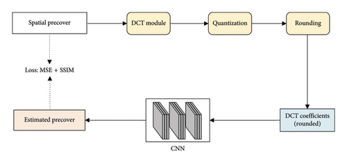
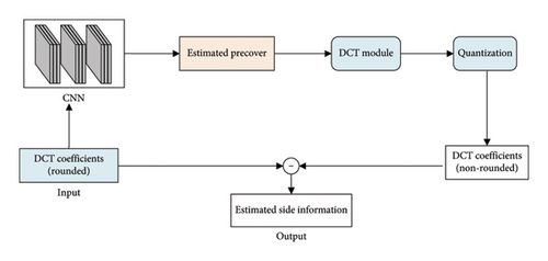
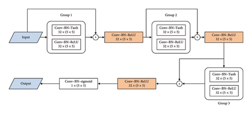
The calculation process of the SI is shown in Figure 4(b). After training the model of the precover estimation network, we can obtain the estimated precover from the input-rounded DCT coefficients and then calculate the nonrounded DCT coefficients. The difference between the rounded DCT coefficients and the DCT coefficients without the rounding operation is used as the SI. The details of the CNN–based precover estimation architecture are shown in Figure 5. It is composed of a series Conv layer, BN layer, and ReLU layer. All the Conv layers employ 5 × 5 kernels with Stride 1.

3.2.2. Adjusting the Embedding Cost

After obtaining the ESI

, the embedding cost of equation (10) is further adjusted according to the amplitude and polarity of the ESI

()

where δ and η are determined by experiments and will be explained in Section 4. Although, the authors in [30] try to use the amplitude of the estimated side formation, the performance was even inferior because inaccurate ESI will make the performance deteriorate. Here, the amplitude

is used for asymmetric adjusting when the absolute value of the SI is smaller than δ. We set the parameter η to a constant to adjust the cost when the absolute value of the SI is larger than δ. Since the large ESI may be inaccurate, only the polarity is used for asymmetric embedding to the SI with a large absolute value.

4. Experimental Results

In this section, we will describe the details of the experimental setup and introduce adaptive learning. Then, we will present the details of adjusting the embedding cost according to the SI. Finally, we will show our experimental results under three different quality factors (QFs) with different payloads.

4.1. Experimental Setup

The experiments were conducted on SZUBase [23], BOSSBase V 1.01 [39], and BOWS2 [40], which contain grayscale images of size 512 × 512. All of the cover images were first resampled to size 256 × 256, and the corresponding quantified DCT matrix was obtained using JPEG transformation with a QF of 75. SZUBase, with 40,000 images, was used to train the JS–GAN and the CNN–based precover estimation model. In the training phase, all parameters of the generator and discriminator were first initialized from a Gaussian distribution. Then, we trained the JS–GAN using the Adam optimizer [32] with a learning rate of 0.0001. The batch size of the input-quantified DCT matrix of the cover image was set to 8.

After a certain number of training iterations, we used the generator and STC encoder [1] to produce the stego images from 20,000 cover images in BOSSBase and BOWS2 for evaluation. Four steganalyzers, including the conventional steganalyzers DCTR [7] and GFR [6], as well as the CNN–based steganalyzer J-XuNet [16] and SRNet [18], were used to evaluate the security performance of JS–GAN. To train the CNN–based steganalyzer, 10,000 cover–stego pairs in BOWS2 and 4000 pairs in BOSSBase were chosen. The other 6000 pairs in BOSSBase were divided into 1000 pairs as the validation set and 5000 pairs for testing. The training stage of JS–GAN was conducted in TensorFlow V 1.11 with an NVIDIA TITAN Xp GPU card.

4.2. The Content-Adaptive Learning of JS–GAN

We trained the JS–GAN for 60 epochs under the target payload of 0.5 bpnzAC and QF 75. The best model according to the attack results with GFR was selected. Then stegos with payloads of 0.1–0.5 bpnzAC were generated by using a STC encoder according to the cost calculated from the best model trained under 0.5 bpnzAC.

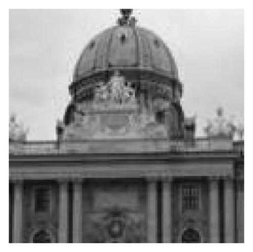
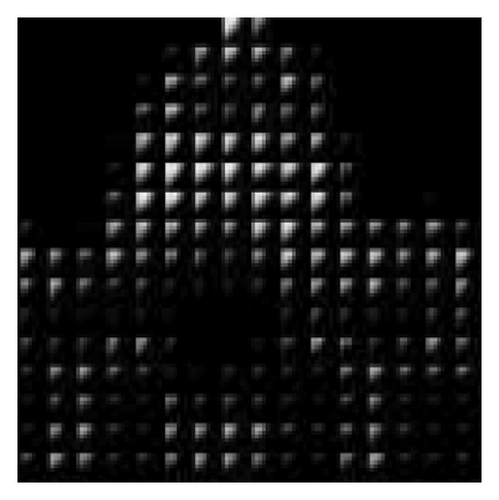
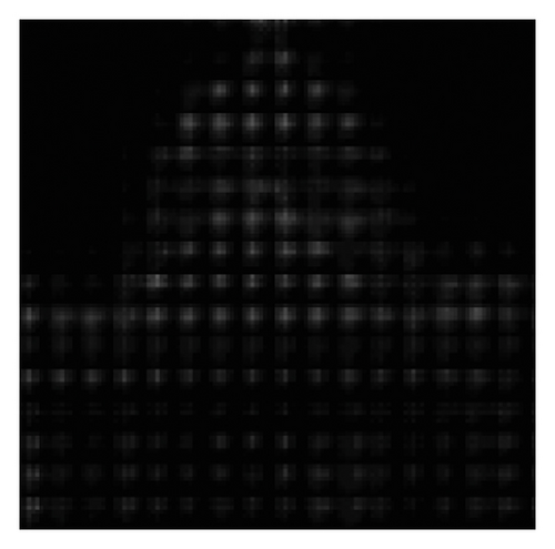
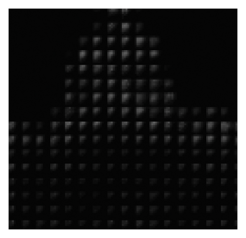
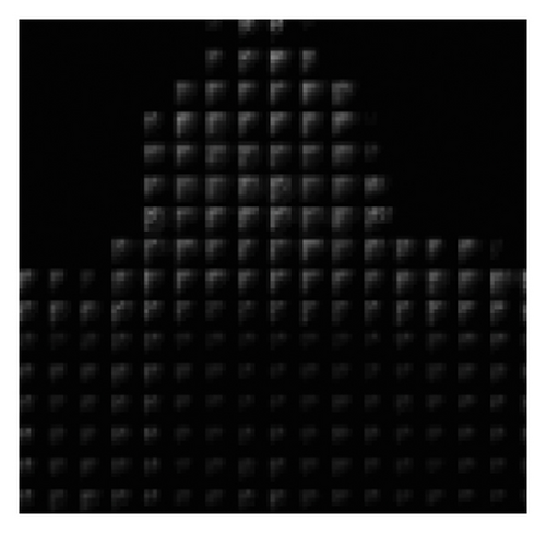
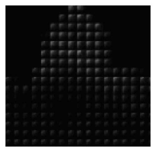
To verify the content-adaptivity of our method, we show the embedding probability map produced by the generator trained after different epochs in Figure 6. The embedding probability generated by J-UNIWARD [2] with the same payload is also given in Figure 6(b) for visual comparison. As shown in Figure 6, the 8 × 8 block property of the embedding probability has been automatically learned. The global adaptability (interblock) and the local adaptability (intrablock) have improved with an increase in the number of training epochs. After 50 training epochs, the block in the complex region has a large embedding probability, which verifies the global adaptability. Inside the 8 × 8 block, the larger probabilities are mostly located in the top left low-frequency region, which proves the local adaptability of JS–GAN. It can be also seen that the embedding probability generated by our GAN–based method has similar characteristics to those generated by J-UNIWARD.

4.3. Parameter Selection for Adjusting the Embedding Cost

We conducted experiments with ESI–aided version JS–GAN (JS–GAN [ESI]) with 0.4 bpnzAC and a QF of 75 to select the proper parameters for asymmetric embedding. The error rate P_E of the steganalyzers is used to quantify the security performance of our proposed framework. The error rate detected by GFR with an ensemble classifier is used to evaluate the performance. First, we investigate the impact of the sign of the ESI . Then, we set the amplitude parameter δ = 0 and observe the effect of the polarity parameter η in equation (26)

The effect of η is shown in Table 1, where η = 1 denotes the original JS–GAN, where the cost of +1 is equal to the cost −1. Experimental results show that the performance would be improved when η decreases. Thus, the performance can be improved by adjusting the cost asymmetrically according to the sign of the ESI. From Table 1, the detection error rate of JS–GAN (ESI) increases by 7.85% with η = 0.65 compared to the original JS–GAN.

Table 1. Error rates of JS–GAN (ESI) with 0.4 bpnzAC detected by GFR under different values of η (δ = 0).

η	0.55	0.6	0.65	0.7	0.75	0.8	1
Error rate	0.2554	0.2607	0.2785	0.2784	0.2758	0.2622	0.2

Note: The best results are highlighted in bold.

After putting η = 0.65, we further investigated the influence of the parameter δ by using the polarity and the amplitude of the SI at the same time. It can be seen from Table 2 that setting δ = 0.05 will achieve better performance than other values; it also can improve the performance about 10% over setting δ = 0.5, which was used in [30]. The experimental results show that only a small amplitude can be used to improve the security performance. This is because amplitudes close to 0.5 are not precise. It can also be seen that setting δ = 0.05 will lead to an improvement by about 3.4% over δ = 0, and this shows that using the amplitude properly can further improve the performance over using only the polarity of the SI. From Tables 1 and 2, we set η = 0.65 and δ = 0.05 for the final version JS–GAN (ESI).

Table 2. Error rates of JS–GAN (ESI) with 0.4 bpnzAC detected by GFR under different values of δ (η = 0.65).

δ	0	0.01	0.05	0.1	0.15	0.2	0.4	0.5
Error rate	0.2785	0.2829	0.3125	0.2969	0.2944	0.2954	0.2799	0.2132

Note: The best results are highlighted in bold.

4.4. Results and Analysis

We selected the classic steganographic algorithms UERD and J-UNIWARD to make a comparison with our proposed methods JS–GAN and JS–GAN (ESI). For a fair comparison, all steganographic algorithms used the STC encoder to embed the messages. Four different steganalyzers were used to evaluate the performance, including the conventional steganalyzers GFR and DCTR, as well as the CNN–based steganalyzers J-XuNet and SRNet.

The experimental results for JPEG-compressed images with QF 75 are shown in Table 3 and Figure 7. From Table 3, it can be seen that under the attack of the conventional steganalyzer GFR, our proposed architecture JS–GAN can obtain better security performance than the conventional methods UERD and J-UNIWARD. For example, under the attack of GFR with 0.4 bpnzAC, the JS–GAN can achieve a better performance by 2.51% and 2.58% than UERD and J-UNIWARD, respectively. Under the attack of the CNN–based steganalyzer SRNet with 0.4 bpnzAC, the proposed JS–GAN can increase the detection error rate by 3.29% and 0.44% over UERD and J-UNIWARD, respectively.

Table 3. Error rates detected by different steganalyzers when QF = 75.

Steganalyzer	Steganographic scheme	Payload
Steganalyzer	Steganographic scheme	0.1 bpnzAC	0.2 bpnzAC	0.3 bpnzAC	0.4 bpnzAC	0.5 bpnzAC
GFR	JS–GAN (ESI)	0.4720	0.4220	0.3707	0.3125	0.2537
	JS–GAN	0.4400	0.3650	0.2826	0.2000	0.1283
	UERD	0.4273	0.3351	0.2468	0.1749	0.1126
	J-UNIWARD	0.4393	0.3488	0.2568	0.1742	0.1090

DCTR	JS–GAN (ESI)	0.4799	0.4474	0.4084	0.3529	0.2848
	JS–GAN	0.4572	0.3916	0.3123	0.2303	0.1528
	UERD	0.4575	0.3871	0.3137	0.2390	0.1690
	J-UNIWARD	0.4655	0.4011	0.3238	0.2492	0.1701

J-XuNet	JS–GAN (ESI)	0.4053	0.3030	0.2232	0.1622	0.1147
	JS–GAN	0.4079	0.2873	0.1859	0.1331	0.0834
	UERD	0.3256	0.1923	0.1122	0.0709	0.0459
	J-UNIWARD	0.3977	0.2750	0.1821	0.1166	0.0752

SRNet	JS–GAN (ESI)	0.3268	0.2142	0.1417	0.0902	0.0618
	JS–GAN	0.3085	0.1867	0.1114	0.0640	0.0292
	UERD	0.1949	0.0865	0.0446	0.0311	0.0143
	J-UNIWARD	0.2971	0.1771	0.1016	0.0596	0.0311

Note: The best results are highlighted in bold.

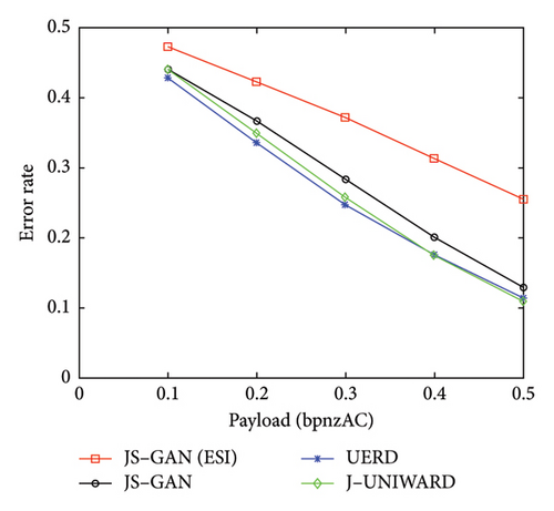
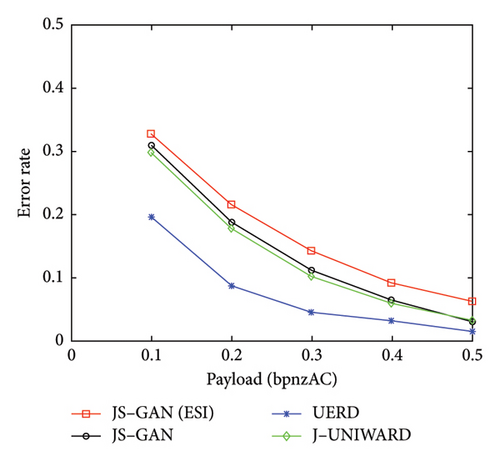
It can be seen from Table 3 that the security performance of JS–GAN can be further improved significantly by incorporating the proposed SI estimated method. With the payload 0.4 bpnzAC, the JS–GAN (ESI) can increase the detection error rate by 11.25% over JS–GAN against the conventional steganalyzer GFR, and it can also increase the detection error rate by 2.62% over JS–GAN to protect against the attack of the CNN–based steganalyzer SRNet. The main reason for the high level of security achieved is mainly because the embedding preserved the statistical characteristics of the precover.

Compared to the conventional methods UERD and J-UNIWARD, a significant improvement can be observed in UERD and J-UNIWARD, respectively. Under the detection of GFR with the payload 0.4 bpnzAC, the detection error of JS–GAN (ESI) is increased by 13.76% and 13.83% over that of UERD and J-UNIWARD, respectively. Under the detection of SRNet with the payload 0.4 bpnzAC, the detection error of JS–GAN (ESI) is also up by 5.91% and 3.06% over UERD and J-UNIWARD, respectively.

To verify the proposed method in the face of different compression QFs, we conducted the experiments for JPEG-compressed images with QFs 50 and 95. The parameters of the generator and discriminator with the QFs 50 and 95 were initialized from the trained best model using the QF 75. The experimental results are shown in Tables 4 and 5, respectively. From Table 4, JS–GAN (ESI) achieves significant improvement compared to the other three steganographic algorithms under the attack of different steganalyzers with different payloads, which proves that the proposed method can achieve better security performance. From Table 5, it can be seen that JS–GAN (ESI) can achieve comparable performance with other steganographic algorithms, and it can also be seen that the performance of JS–GAN (ESI) for higher QF needs to be further improved.

Table 4. Error rates detected by different steganalyzers when QF = 50.

Steganalyzer	Steganographic scheme	Payload
Steganalyzer	Steganographic scheme	0.1 bpnzAC	0.2 bpnzAC	0.3 bpnzAC	0.4 bpnzAC	0.5 bpnzAC
GFR	JS–GAN (ESI)	0.4596	0.4067	0.3392	0.2730	0.2119
	JS–GAN	0.4222	0.3243	0.2322	0.1524	0.0937
	UERD	0.4110	0.3100	0.2181	0.1421	0.0899
	J-UNIWARD	0.4151	0.3104	0.2029	0.1277	0.0735

DCTR	JS–GAN (ESI)	0.4688	0.4210	0.3604	0.3036	0.2483
	JS–GAN	0.4304	0.3360	0.2431	0.1620	0.0982
	UERD	0.4363	0.3560	0.2696	0.1918	0.1287
	J-UNIWARD	0.4386	0.3571	0.2710	0.1837	0.1211

J-XuNet	JS–GAN (ESI)	0.4049	0.2990	0.2144	0.1563	0.1104
	JS–GAN	0.3701	0.2466	0.1589	0.0977	0.0647
	UERD	0.2983	0.1630	0.0952	0.0554	0.0345
	J-UNIWARD	0.3764	0.2361	0.1441	0.0861	0.0514

SRNet	JS–GAN (ESI)	0.3266	0.2154	0.1262	0.0804	0.0474
	JS–GAN	0.2702	0.1491	0.0781	0.0377	0.0188
	UERD	0.1764	0.0782	0.0408	0.0182	0.0178
	J-UNIWARD	0.2808	0.1402	0.0732	0.0377	0.0334

Note: The best results are highlighted in bold.

Table 5. Error rates detected by different steganalyzers when QF = 95.

Steganalyzer	Steganographic scheme	Payload
Steganalyzer	Steganographic scheme	0.1 bpnzAC	0.2 bpnzAC	0.3 bpnzAC	0.4 bpnzAC	0.5 bpnzAC
GFR	JS–GAN (ESI)	0.4817	0.4525	0.4122	0.3652	0.3095
	JS–GAN	0.4783	0.4434	0.3920	0.3382	0.2634
	UERD	0.4754	0.4268	0.3702	0.3072	0.2423
	J-UNIWARD	0.4894	0.4549	0.4033	0.3417	0.2791

DCTR	JS–GAN (ESI)	0.4868	0.4653	0.4295	0.3859	0.3348
	JS–GAN	0.4864	0.4599	0.4150	0.3604	0.2877
	UERD	0.4888	0.4597	0.4261	0.3697	0.3093
	J-UNIWARD	0.4953	0.4750	0.4450	0.3984	0.3430

J-XuNet	JS–GAN (ESI)	0.4706	0.4118	0.3340	0.2615	0.1811
	JS–GAN	0.4752	0.4258	0.3441	0.2735	0.1893
	UERD	0.4295	0.3358	0.2380	0.1773	0.1174
	J-UNIWARD	0.4841	0.4434	0.3988	0.3309	0.2689

SRNet	JS–GAN (ESI)	0.4344	0.3125	0.2103	0.1364	0.0779
	JS–GAN	0.4267	0.3043	0.2062	0.1286	0.0723
	UERD	0.3201	0.1980	0.1167	0.0673	0.0478
	J-UNIWARD	0.4349	0.3250	0.2347	0.1599	0.1008

Note: The best results are highlighted in bold.

5. Conclusion

In this paper, an automatically embedding cost function learning framework called JS–GAN has been proposed for JPEG image steganography. Our experimental results obtained by conventional and CNN–based steganalyzers allow us to draw the following conclusions:

1.
Through an adversarial training between the generator and discriminator, an automatic content-adaptive steganography algorithm can be designed for the JPEG domain. Compared to the conventional heuristically designed JPEG steganography algorithms, the automatic learning method can adjust the embedding strategy flexibly according to the characteristics of the steganalyzer.
2.
To simulate the message embedding and avoid the gradient-vanishing problem, a gradient-descent–friendly and highly efficient probability-based embedding simulator can be designed. Experimental results show that the probability-based embedding simulator can contribute to learning the local and global adaptivity.
3.
When the original uncompressed image is not available, a properly trained CNN–based SI estimation model can acquire the ESI. The security performance can be further improved dramatically by using asymmetric embedding with the well ESI.

This paper opens up a promising direction in embedding cost learning in the JPEG domain by adversarial training between the generator and the discriminator. It also shows that predicting the SI brings a significant improvement when only the JPEG-compressed image is available. Further investigation could include the following aspects. First, higher efficiency generators and discriminators can be further investigated. Second, the conflict with the gradient-vanishing and simulating the embedding process also have much room for improvement. Third, we have only carried out an initial study using the CNN to estimate the SI, and the asymmetric adjusting strategy deserves further research. Finally, we will further improve the performance under the larger QF 95.

Disclosure

This paper is already published in the pre-print given in the below link “https://arxiv.org/abs/2107.13151” [41].

Conflicts of Interest

The authors declare no conflicts of interest.

Funding

This work was supported in part by the NSFC under Grant no. 62102462/62102100, the Guangdong Basic and Applied Basic Research Foundation under Grant no. 2022A1515010108, the Key Research Platforms and Projects of Universities in Guangdong Province under Grant no. 2024ZDZX1038, and the Research Project ofthe Guangdong Polytechnic Normal University under Grant no. 2021SDKYA127/2022SDKYA027.

Acknowledgments

This work was supported in part by the NSFC under Grant no.62102462/62102100, the Guangdong Basic and Applied Basic Research Foundation under Grant no. 2022A1515010108, the Key Research Platforms and Projects of Universities in Guangdong Province under Grant no. 2024ZDZX1038, and the Research Project of Guangdong Polytechnic Normal University under Grant no. 2021SDKYA127/2022SDKYA027.

Open Research

Data Availability Statement

The data that support the findings of this study are available in BOSS-Base v1.01 at https://dde.binghamton.edu/download/, reference number [39].

References

1 Filler T., Judas J., and Fridrich J., Minimizing Additive Distortion in Steganography Using Syndrome-Trellis Codes, IEEE Transactions on Information Forensics and Security. (2011) 6, no. 3, 920–935.
10.1109/TIFS.2011.2134094
Web of Science® Google Scholar
2 Holub V., Fridrich J., and Denemark T., Universal Distortion Function for Steganography in an Arbitrary Domain, EURASIP Journal on Information Security. (2014) 2014, no. 1, 1–13.
10.1186/1687-417X-2014-1
Google Scholar
3 Guo L., Ni J., Su W., Tang C., and Shi Y., Using Statistical Image Model for JPEG Steganography: Uniform Embedding Revisited, IEEE Transactions on Information Forensics and Security. (2015) 10, no. 12, 2669–2680.
10.1109/TIFS.2015.2473815
Web of Science® Google Scholar
4 Liu Q., Su W., Ni J., Hu X., and Huang J., An Efficient Distortion Cost Function Design for Image Steganography in Spatial Domain Using Quaternion Representation, Signal Processing. (2024) 219.
10.1016/j.sigpro.2023.109370
Web of Science® Google Scholar
5 Su W., Ni J., Hu X., and Li B., Efficient Audio Steganography Using Generalized Audio Intrinsic Energy With Micro-Amplitude Modification Suppression, IEEE Transactions on Information Forensics and Security. (2024) 19, 6559–6572.
10.1109/TIFS.2024.3417268
Web of Science® Google Scholar
6 Song X., Liu F., Yang C., Luo X., and Zhang Y., Steganalysis of Adaptive Jpeg Steganography Using 2d Gabor Filters, Proceedings of the 3rd ACM Workshop on Information Hiding and Multimedia Security, ser. IaH&MMSec ’15, June 2015, New York, NY, 15–23.
Google Scholar
7 Holub V. and Fridrich J., Low-Complexity Features for Jpeg Steganalysis Using Undecimated DCT, IEEE Transactions on Information Forensics and Security. (2015) 10, no. 2, 219–228.
10.1109/TIFS.2014.2364918
Web of Science® Google Scholar
8 Kodovsky J., Fridrich J., and Holub V., Ensemble classifiers for Ste- Ganalysis of Digital Media, IEEE Transactions on Information Forensics and Security. (2012) 7, no. 2, 432–444.
10.1109/TIFS.2011.2175919
Web of Science® Google Scholar
9 Denemark T. D., Boroumand M., and Fridrich J., Steganalysis Features for Content-Adaptive Jpeg Steganography, IEEE Transactions on Information Forensics and Security. (2016) 11, no. 8, 1736–1746.
10.1109/TIFS.2016.2555281
Web of Science® Google Scholar
10 Tang W., Li H., Luo W., and Huang J., Adaptive Steganalysis Based on Embedding Probabilities of Pixels, IEEE Transactions on Information Forensics and Security. (2015) 11, no. 4, 734–745.
10.1109/TIFS.2015.2507159
Web of Science® Google Scholar
11 Tan S. and Li B., Stacked Convolutional Auto-Encoders for Steganal- Ysis of Digital Images, Proceedings of the Signal and Information Processing Association Annual Summit and Conference (APSIPA), 2014 Asia-Pacific, December 2014, Chiang Mai, Thailand, 1–4.
Google Scholar
12 Qian Y., Dong J., Wang W., and Tan T., Deep Learning for Steganalysis via Convolutional Neural Networks, 9409, Proceedings of SPIE Media Watermarking, Security, and Forensics 2015, Part of SPIE/IS&T Annual.Symposium on Electronic Imaging, March 2015, San Francisco, CA.
Google Scholar
13 Yedroudj M., Comby F., and Chaumont M., Yedroudj-Net: An efficient CNN for Spatial Steganalysis, Proceedings of the 2018 IEEE International Conference on Acoustics, Speech and Signal Processing (ICASSP), April 2018, Alberta, Canada, 2092–2096.
Google Scholar
14 Ye J., Ni J., and Yi Y., Deep Learning Hierarchical Representations for Image Steganalysis, IEEE Transactions on Information Forensics and Security. (2017) 12, no. 11, 2545–2557.
10.1109/TIFS.2017.2710946
Web of Science® Google Scholar
15 Zeng J., Tan S., Li B., and Huang J., Large-Scale Jpeg Image Ste- Ganalysis Using Hybrid Deep-Learning Framework, IEEE Transactions on Information Forensics and Security. (2018) 13, no. 5, 1200–1214.
10.1109/TIFS.2017.2779446
Web of Science® Google Scholar
16 Xu G., Deep Convolutional Neural Network to Detect J-UNIWARD, Proceedings of the 5th ACM Workshop on Information Hiding and Multimedia Security, ser. IH&MMSec ’17, June 2017, New York, NY, 67–73.
Google Scholar
17 Yang J., Kang X., Wong E., and Shi Y., Jpeg Steganalysis With Combined Dense Connected CNNs and SCA-GFR, Multimedia Tools and Applications. (2019) 78, no. 7, 8481–8495.
10.1007/s11042-018-6878-4
Web of Science® Google Scholar
18 Boroumand M., Chen M., and Fridrich J., Deep Residual Network for Steganalysis of Digital Images, IEEE Transactions on Information Forensics and Security. (2019) 14, no. 5, 1181–1193.
10.1109/TIFS.2018.2871749
Web of Science® Google Scholar
19 Baluja S., Hiding Images in Plain Sight: Deep Steganography, Advances in Neural Information Processing Systems, 2017, 30, Curran Associates, Inc.
Google Scholar
20 Yang J., Shang F., Liao Y., and Chen Y., Toward High Capacity and Robust JPEG Steganography Based on Adversarial Training, Security and Communication Networks. (2023) no. 1.
10.1155/2023/3813977
Google Scholar
21 Shang F., Lan Y., Yang J., Li E., and Kang X., Robust Data Hiding for JPEG Images With Invertible Neural Network, Neural Networks. (2023) 163, 219–232.
10.1016/j.neunet.2023.03.037
PubMed Web of Science® Google Scholar
22 Su W., Ni J., and Sun Y., StegaStyleGAN: Towards Generic and Practical Generative Image Steganography, AAAI Conference on Artificial Intelligence. (2024) 38, no. 1, 240–248.
10.1609/aaai.v38i1.27776
Google Scholar
23 Tang W., Tan S., Li B., and Huang J., Automatic Steganographic Distortion Learning Using a Generative Adversarial Network, IEEE Signal Processing Letters. (2017) 24, no. 10, 1547–1551.
10.1109/LSP.2017.2745572
Web of Science® Google Scholar
24 Yang J., Ruan D., Huang J., Kang X., and Shi Y., An Embedding Cost Learning Framework Using GAN, IEEE Transactions on Information Forensics and Security. (2019) 15, 839–851.
10.1109/TIFS.2019.2922229
Web of Science® Google Scholar
25 Tang W., Li B., Barni M., Li J., and Huang J., An Automatic Cost Learning Framework for Image Steganography Using Deep Reinforcement Learning, IEEE Transactions on Information Forensics and Security. (2020) 16, 952–967.
10.1109/TIFS.2020.3025438
Web of Science® Google Scholar
26 Ronneberger O., Fischer P., and Brox T., U-Net: Convolutional Networks for Biomedical Image Segmentation, Proceedings of the Medical Im- Age Computing and Computer-Assisted Intervention (MICCAI), October 2015, Munich, Germany, 234–241.
Google Scholar
27 Yang J., Ruan D., Kang X., and Shi Y., Towards Automatic Embedding Cost Learning for Jpeg Steganography, Proceedings of the ACM Workshop on Information Hiding and Multimedia Security, July 2019, Paris, France, 37–46.
Google Scholar
28 Ker A. D., A Fusion of Maximum Likelihood and Structural Steganalysis, International Workshop on Information Hiding, 2007, Springer, 204–219.
10.1007/978-3-540-77370-2_14
Google Scholar
29 Denemark T. and Fridrich J., Side-informed Steganography with Addi- Tive Distortion, 2015 IEEE International Workshop on Information Forensics and Security (WIFS), November 2015, Rome, Italy, IEEE, 1–6.
Google Scholar
30 Li W., Chen K., Zhang W., Zhou H., Wang Y., and Yu N., Jpeg Steganography with Estimated Side-Information, IEEE Transactions on Circuits and Systems for Video Technology. (July 2020) 30, no. 7, 2288–2294.
10.1109/TCSVT.2019.2925118
Web of Science® Google Scholar
31 Filler T. and Fridrich J., Gibbs Construction in Steganography, IEEE Transactions on Information Forensics and Security. (December 2010) 5, no. 4, 705–720.
10.1109/TIFS.2010.2077629
Web of Science® Google Scholar
32 Kingma D. and Ba J., Adam: A Method for Stochastic Optimization, Computer Science. (2014) .
Google Scholar
33 Sedighi V., Cogranne R., and Fridrich J., Content-Adaptive Steganog- Raphy by Minimizing Statistical Detectability, IEEE Transactions on Information Forensics and Security. (February 2016) 11, no. 2, 221–234.
10.1109/TIFS.2015.2486744
Web of Science® Google Scholar
34 Li B., Tan S., Wang M., and Huang J., Investigation on Cost Assignment in Spatial Image Steganography, IEEE Transactions on Information Forensics and Security. (2014) 9, no. 8, 1264–1277.
10.1109/TIFS.2014.2326954
Web of Science® Google Scholar
35 Pevn´y T., Filler T., and Bas P., R. Bohme, P. W. L. Fong, and R. Safavi-Naini, Using High-Dimensional Image Models to Perform Highly Undetectable Steganography, Proceedings of the International Workshop on Information Hiding, 2010, Springer, Berlin, Germany, 161–177.
10.1007/978-3-642-16435-4_13
Google Scholar
36 Holub V. and Fridrich J., Designing Steganographic Distortion Using Directional Filters, Proceedings of the 2012 IEEE International Workshop on Information Forensics and Security (WIFS), December 2012, Tenerife, Spain, 234–239.
Google Scholar
37 Li B., Wang M., Huang J., and Li X., A New Cost Function for Spatial Image Steganography, Proceedings of the 2014 IEEE International Conference on Image Processing (ICIP), October 2014, Paris, France, 4206–4210.
Google Scholar
38 Fridrich J. and Filler T., Practical Methods for Minimizing Embedding Impact in Steganography, Proceedings of Spie the International Society for Optical Engineering. (2007) 6505.
Google Scholar
39 Bas P., Filler T., and Pevn T., Break Our Steganographic System”: The Ins and Outs of Organizing Boss, Proceedings of the 13th International Conference on Information Hiding, May 2011, Springer, Berlin, 59–70.
Google Scholar
40 Bas P. and Furon T., Bows-2, 2007, http://bows2.ec-lille.fr.
Google Scholar
41 Yang J., Liao Y., Shang F., Kang X., and Shi Y., JPEG Steganography With Embedding Cost Learning and Side-Information Estimation, 2021, https://arxiv.org/abs/2107.13151.
Google Scholar

All articles

JPEG Image Steganography With Automatic Embedding Cost Learning

Abstract

1. Introduction