International Journal of Intelligent Systems

Volume 2025, Issue 1 5010973

Research Article

Open Access

Intelligent Sensing and Identification of Spectrum Anomalies With Alpha-Stable Noise

Mingqian Liu,

Mingqian Liu

orcid.org/0000-0001-9872-9710

State Key Laboratory of Integrated Service Networks , Xidian University, Shaanxi , Xi’an , 710071 , China

Search for more papers by this author

Zhaoxi Wen,

Corresponding Author

Zhaoxi Wen

[email protected]

orcid.org/0009-0008-3577-9858

State Key Laboratory of Integrated Service Networks , Xidian University, Shaanxi , Xi’an , 710071 , China

Search for more papers by this author

Yunfei Chen,

Yunfei Chen

orcid.org/0000-0001-8083-1805

Department of Engineering , University of Durham , Durham , UK DH1 3LE , China , dur.ac.uk

Search for more papers by this author

Junlin Zhang,

Junlin Zhang

State Key Laboratory of Integrated Service Networks , Xidian University, Shaanxi , Xi’an , 710071 , China

Search for more papers by this author

Huigui Cheng,

Huigui Cheng

State Key Laboratory of Integrated Service Networks , Xidian University, Shaanxi , Xi’an , 710071 , China

Search for more papers by this author

Nan Zhao,

Nan Zhao

orcid.org/0000-0002-5624-080X

School of Information and Communication Engineering , Dalian University of Technology , Dalian , 116024 , China , dlut.edu.cn

Search for more papers by this author

Mingqian Liu,

Mingqian Liu

orcid.org/0000-0001-9872-9710

State Key Laboratory of Integrated Service Networks , Xidian University, Shaanxi , Xi’an , 710071 , China

Search for more papers by this author

Zhaoxi Wen,

Corresponding Author

Zhaoxi Wen

[email protected]

orcid.org/0009-0008-3577-9858

State Key Laboratory of Integrated Service Networks , Xidian University, Shaanxi , Xi’an , 710071 , China

Search for more papers by this author

Yunfei Chen,

Yunfei Chen

orcid.org/0000-0001-8083-1805

Department of Engineering , University of Durham , Durham , UK DH1 3LE , China , dur.ac.uk

Search for more papers by this author

Junlin Zhang,

Junlin Zhang

State Key Laboratory of Integrated Service Networks , Xidian University, Shaanxi , Xi’an , 710071 , China

Search for more papers by this author

Huigui Cheng,

Huigui Cheng

State Key Laboratory of Integrated Service Networks , Xidian University, Shaanxi , Xi’an , 710071 , China

Search for more papers by this author

Nan Zhao,

Nan Zhao

orcid.org/0000-0002-5624-080X

School of Information and Communication Engineering , Dalian University of Technology , Dalian , 116024 , China , dlut.edu.cn

Search for more papers by this author

First published: 20 February 2025

https://doi.org/10.1155/int/5010973

Academic Editor: Weiwei Jiang

Share a link

Email
Wechat
Bluesky

Abstract

As the electromagnetic environment becomes more complex, a significant number of interferences and malfunctions of authorized equipment can result in anomalies in spectrum usage. Utilizing intelligent spectrum technology to sense and identify anomalies in the electromagnetic space is of great significance for the efficient use of the electromagnetic space. In this paper, a method for intelligent sensing and identification of anomalies in spectrum with alpha-stable noise is proposed. First, we use a delayed feedback network (DFN) to suppress alpha-stable noise. Then, we use a long short-term memory (LSTM) autoencoder-based attention mechanism to sense anomaly. Finally, we use the deep forest model to identify abnormal spectrum. Simulation results demonstrate that the proposed method effectively suppresses alpha-stable noise, and it outperforms existing methods in abnormal spectrum sensing and identification.

1. Introduction

In recent years, with the rapid development and globalization of new technologies, such as the cloud computing [1–6], Internet of Things (IoT) [7–12], smart cities [13–15], Internet of Vehicles (IoVs) [16], and the wide application of radio communication technology [17], spectrum resources have become increasingly scarce [18–22]. To improve usage, spectrum resources can be used by other users when the current spectrum is idle. However, there are various issues associated with the unregulated use of spectrum resources, such as abnormal spectrum. In the meantime, the emergence of radio interference may also bring potential threats to the regular communication services, causing anomalies in the spectrum signals. Many factors can lead to anomalies in the spectrum. For example, when the authorized useful radio signal is sent from the wireless transmitter, the out-of-band radiation will be generated. For nearly receivers, this out-of-band interference signal can lead to in-band blocking of the receiver and cause errors in the received information [23]. Others include channel interference, adjacent channel interference, intermodulation interference, and blocking interference [24]. When the technical indicators of the communication equipment do not meet regulatory requirements, it may fail to work. These factors will generate spectrum anomalies, including equipment failure and stray radiation exceeding the standard [25]. These abnormal spectrum signals will affect the monitoring of spectrum resources and lead to confusion in the management of radio spectrum resources. Therefore, it is necessary to comprehensively and effectively manage spectrum resources using abnormal spectrum sensing and identification. In this way, we can prevent legitimate frequency bands from being illegally used by malicious users, avoid interference from external signals, and meet the needs of most users. Moreover, in the complex electromagnetic environment, both human and natural factors will lead to the generation of non-Gaussian noise, and we use alpha-stable noise to describe this kind of noise, which is studied in this paper. In addition, alpha-stable noise has impulsive characteristics with the spike pulse.

Regarding abnormal spectrum sensing, the authors in [26] proposed an unsupervised spectrum anomaly sensing approach with explainable features based on the adversarial autoencoder (AAE). During training, it does not require manual labeling of a large number of sample data, and the power spectral density (PSD) spectrum of the signal was extracted as explainable features. When the false alarm probability was 1%, the model achieved an average abnormal sensing accuracy of over 80%. Reference [27] proposed a radio anomaly sensing algorithm based on improved generative adversarial network (GAN). First, short-time Fourier transform (STFT) was applied to obtain the spectrogram from the received signal. Subsequently, the spectrogram was reconstructed by integrating the encoder network into the original GAN. The presence of anomalies can be sensed based on the reconstruction error and discriminator loss. Reference [28] proposed a spectrum sensing method based on the GAN model for many radio interference situations in wireless communication systems. It can be used for sensing abnormal spectrum with impulsive noise.

In the study of abnormal spectrum identification, the authors in [29] proposed an interference classification and identification algorithm based on signal feature space and support vector machine (SVM). It used signal model expression and signal space theory to extract the bandwidth, spatial power spectrum flatness, spatial spectrum peak-to-average ratio, and other characteristics of interference signals. In addition, it combined the SVM method to classify the interference signal samples. Reference [30] proposed a classification algorithm for studying interference signals in the global navigation system. The model consisted of an interference fingerprint spectrum and a convolutional neural network (CNN). The interference fingerprint spectrum can be used to learn the frequency and power distribution of interference signals. At a low interference power of −95dBm, the identification accuracy of nine interference anomaly types can reach more than 90%. Reference [31] proposed a wireless interference classification algorithm based on the time-frequency (TF) component analysis of CNN, which allowed convolutional computation to be performed only in the position where TF components or important parts exist in the TF image of the interfered signal, thus reducing redundant computation. Compared with traditional CNN, the computational complexity of the method was reduced by about 75% while slightly improving the identification accuracy. Reference [32] proposed a learning framework based on long short-term memory (LSTM) denoising autoencoder, which automatically extracted signal features from noisy radio signals and used the learned features to classify the type of modulated signal. The classification of real-world radio data showed that the proposed framework can reliably and efficiently classify the received radio signals.

From the above, we can know that in traditional abnormal spectrum sensing methods, the sensing threshold is often set based on empirical knowledge. However, this threshold is subject to human factors, leading to significant misjudgments in the final sensing results. In general, the initial consideration is to use deep neural networks (DNNs) to address the entire classification problem. However, DNN often requires a large number of training parameters and encounter challenges related to excessive hyperparameter settings. Recurrent neural network (RNN) variants such as gated recurrent unit (GRU) and bidirectional LSTM have their own defects in the scenario of this paper, such as insufficient parameter complexity of GRU and long training time of bidirectional LSTM. Therefore, none of them can complete the task of this paper well. To solve these issues, we propose the abnormal spectrum intelligent sensing and identification method with alpha-stable noise in this paper. This method can effectively suppress alpha-stable noise and has better performance than existing methods. The main contributions of this paper can be summarized as follows:

•
To suppress the disturbance of alpha-stable noise to the intelligent sensing and identification of abnormal spectrum, a delayed feedback network (DFN) is used;
•
The characteristics of several proposed abnormal spectrum types are analyzed, and the feature extraction of the abnormal spectrum types is completed;
•
The LSTM autoencoder based on attention mechanism is used to sense abnormal spectrum;
•
The deep forest model is used to identify abnormal spectrum.

The remainder of this paper is organized as follows. Section 2 gives the system model. Section 3 proposes the method for abnormal spectrum intelligent sensing and identification. In Section 4, the simulations results are presented. Finally, the conclusion is given in Section 5.

2. System Model

2.1. Spectrum Sensing Model

Figure 1 shows the multiantenna collaborative spectrum sensing scenario. From Figure 1, it can be seen that the sensing model consists of a primary user (PU), L secondary users (SUs), and a fusion center. The transmitter of the PU has M antennas, and the receiver at the SU has K antennas. At the nth sampling time, the received signal at the dth SU can be expressed as

()

where H₁ and H₀ indicate the presence and absence of PU signals, respectively.

, y_d,m(n) and w_d,m(n) represent the signal and noise received by the m th antenna at the d th SU in the n th sampling time, respectively, s(n) denotes the signal transmitted by the c th antenna at the n th sampling time with

and n = 0, 1, …, N − 1, and N is the total number of sampling points of the signal. h_d(n) = [h_d,1(n), …, h_d,m(n), …, h_d,K(n)], h_d,m(n) stands for the channel response on the m th receiving antenna.

Details are in the caption following the image — **Figure 1**
Open in figure viewer PowerPoint

Spectrum sensing scene.

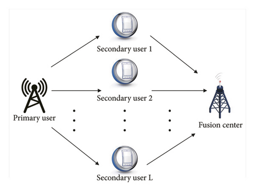
In this paper, we use the Rayleigh fading channel as the wireless fading channel with , that is, the real and imaginary parts of h_d(n) are independent and follow the same Gaussian distribution with a mean of zero and a variance of . So, h_d(n) follows a complex Gaussian distribution with a mean of zero.

2.2. Noise Model

In this paper, we use the alpha-stable noise as the noise model. Alpha-stable noise is introduced to simulate the noise signal with short-term large values encountered in the actual communication environment. Its characteristic function expression is expressed as follows:

()

where

()

where sign(t) denotes the symbolic function. The alpha stable distribution is determined by the parameters α, μ, γ, and β. α represents the characteristic exponent with 0 < α < 2. The larger the α is, the thinner the stable distribution will be. μ denotes the symmetric parameter with −1 ≤ μ ≤ 1. When μ = 0, the stable distribution is symmetric. γ is the scale parameter with γ ≥ 0. β stands for the position parameter with −∞ < β < +∞, and the shift of the probability density function (P.D.F.) of the stable distribution on the x axis is determined by this parameter. In this paper, we set μ = 0, β = 0, and γ = 1, which is symmetric alpha stable (SαS) distribution, and we set 1 ≤ α ≤ 2.

Since it is difficult to obtain the second order moment of alpha-stable noise, the generalized signal-to-noise ratio (GSNR) is used in this paper to replace the traditional signal-to-noise ratio (SNR). The GSNR is given by

()

where

stands for the variance of the signal.

3. Abnormal Spectrum Intelligent Sensing and Identification

3.1. Alpha-Stable Noise Suppression

DFN is a type of neural network that enhances the reservoir layer of the traditional pooling computing model. Its delayed network with feedback systems generates short-term dynamic memory, allowing the network to replicate transient neural responses. Based on this characteristic, non-Gaussian noise can be suppressed. Therefore, we use DFN to suppress alpha-stable noise in this paper.

The first layer of the DFN is the input layer, where a time encoder is applied to encode the information fed into the network. In this paper, a non-Gaussian noise sequence w(k) is added to the input of the DFN. The second layer is the reservoir layer, which consists of a single nonlinear node and a delay ring. It calculates the reservoir layer state through w(k − (τ/N)(N − i)), 1 ≤ i ≤ k as

()

The third layer is the output layer, which can be expressed as

()

where x(k) is the input state vector, w_i denotes the weight of the state, N stands for the number of neurons in the DFN, and τ represents the delay length. One has

from the abovementioned training process, where

is the output noise vector and † denotes the Moore–Penrose generalized inverse matrix. The purpose of the training is to ensure that the weighted sum of the states is close to the target output value. After the network training is complete, the received signal x(k) with noise is added to the DFN input side. The predicted noise sequence

is obtained at the output side by weighting the states. At this time, we perform cancellation processing using x(k), where

is canceled out. The signal after noise suppression is

3.2. Abnormal Spectrum Intelligent Sensing

3.2.1. Analysis and Modeling of Abnormal Spectrum States

In the electromagnetic environment, after using spectrum sensing technology to sense the authorized PU signal mixed with non-Gaussian noise, we need to promptly monitor the identified PU signal to determine if its current working state is normal. This process is known as abnormal spectrum sensing. In this paper, we study four types of abnormal spectrum, namely, signal interrupt transmission, frequency shift emission, power exceeding standard, and equipment failure. First, we extract the characteristics of the abnormal spectrum states mentioned above and then construct an LSTM autoencoder based on an attention mechanism to complete the abnormal spectrum intelligent sensing.

The signal interrupt transmission means that the actual working frequency of the monitoring signal does not exceed the defined frequency range limit, and its working bandwidth does not exceed the specified range. However, the signal’s actual emission level is lower than the emission level recorded in the authorized signal history spectrum database. The expression of signal interrupt transmission is given by

()

where f_s denotes the actual working frequency of X, X is the monitoring signal, U_s represents the working level of X, and f stands for the working frequency of the signal in the obtained authorized signal historical spectrum database. R, B, and U denote the frequency jitter range, the working bandwidth, and the signal level of the historical data, respectively.

The frequency shift emission implies that the working bandwidth of the monitoring signal does not exceed the upper and lower limits of the specified bandwidth range, while the actual working frequency of the signal falls outside the specified frequency jitter range. The expression of the frequency shift emission is expressed as

()

The power exceeding standard means that the actual working frequency of the monitoring signal is within the frequency jitter value allowed by the authorized signal. The range of its working frequency does not exceed the bandwidth requirement of the authorized signal frequency point. But the actual transmitting power of the signal is 5–10 times higher than the obtained signal transmitting power in the historical spectrum database of the authorized signal. The formula of the power exceeding standard is expressed as

()

The equipment failure refers to the wear or corrosion of equipment caused by external forces during the working process, resulting in the functional damage to the equipment. The occurrence of such damage may cause problems in the starting process of the equipment and may also be accompanied by abnormal vibration phenomena, making it challenging for the equipment to meet the specified technical requirements.

3.2.2. Intelligent Characterization of Abnormal Spectrum

In this paper, the intelligent representations of the abnormal spectrum include time occupancy, frequency shift disturbance sequence, relative wavelet time entropy, and Mahalanobis distance.

Time occupancy refers to measuring the duration that a specific channel is present within a designated frequency band or frequency point during a monitoring period. This metric indicates whether the monitored frequency band is actively in use or idle. The time occupancy is defined as follows:

()

where T_u denotes the time of the current channel in occupied state, T_f is the time of the current channel in idle state, and T represents the total monitoring time. The longer the monitoring time, the shorter the sampling time slot, resulting in more time occupancy data being collected, which better reflects the channel occupancy.

The frequency shift disturbance sequence refers to the ratio of the number of observed signal points within a specified frequency disturbance range to the total number of observed signal points in a particular time and space range. The definition is given by

()

where C_u represents the total number of observed signal points, and C_a denotes the number of observed signal points whose working frequency band does not exceed the specified frequency disturbance range. Therefore, we can obtain [f_si, f_ei] ⊂ [f₁, f₂], or the working frequency band of the ith signal point is a subset of the specified frequency disturbance range.

When the power exceeding the standard value during use, the working power of the authorized signal will be much larger than the normal working power. To characterize this kind of abnormal spectrum, the relative wavelet time entropy parameter is introduced. For the received signal f(t), its discrete wavelet transform can be defined as

()

where

denotes the complex conjugate function of Ψ_j,k(t) and the discrete base wavelet. For ease of calculation, we take the binary wavelet sampling calculation, that is, Ψ_j,k(t) = 2^−(j/2)Ψ(2^−jt − k), j ∈ Z, k ∈ Z, and d_j(k) represents the kth wavelet coefficient on the jth scale. Assuming that the discrete wavelet decomposition scale of the received signal is N, the wavelet energy on the jth scale can be given by

()

According to the property of orthogonal wavelet transform, the total energy is equal to the sum of the wavelet energy at all scales, then we have

()

To characterize the energy distribution of the signal in TF space, the wavelet Shannon entropy of f(t) is defined as

()

where p_j denotes the relative wavelet energy on the jth scale with p_j = e_j/e_total, and ∑_jp_j = 1. Based on the wavelet entropy analysis above, a sliding window is incorporated to investigate the evolution of signal wavelet entropy over time scales. Let the width of the sliding window defined on this wavelet coefficient be w and the time segment divided be M. Then, the wavelet energy in the ith sliding window on the jth scale is expressed as

()

Then, the total energy of the wavelet under the ith window is equal to the sum of the component energies under the decomposition of various scales, so we can obtain

()

and when the monitoring spectrum has the power exceeding standard, the wavelet entropy of the signal will change significantly. Assuming that the relative wavelet energy of the two segments before and after the sampled signal is p_j and q_j, respectively, and the sum of p_j and q_j is 1, the sliding window is introduced to analyze the change in the relative wavelet entropy of the two segments before and after the signal on the time scale, and the relative wavelet time entropy can be defined as

()

During the use of radio signal transmitting equipment, various problems may arise. To describe the spectrum using authorized signals in the monitoring period of the specified working frequency band, the Mahalanobis distance parameter is introduced. The main idea of this parameter is to calculate the similarity between two sets of feature samples. It takes into account the subtle connections between the different features of the sample. If we consider the frequency dimension, the sampled spectrum data are correlated in this dimension, and the expression of the Mahalanobis distance is expressed as

()

where the sample data

denote a set of signal field strength values over the entire working frequency band at the current observation time slot with

, k stands for the subscript cutoff value of the frequency band range,

represents a set of signal field strength values over the entire working frequency band for n consecutive days in the past historical period under the current observation time slot, the dimension of s_i is k, and the mean vector of S is

and μ_i = (y_1i + y_2i + ⋯+y_ni)/n, i = 1, 2, …, k. It means that in the specified frequency band, the mean vector

can be obtained by analyzing the statistical data of signal field intensity for n consecutive days throughout the historical period and then the resulting value is adjusted based on the number of days.

3.2.3. LSTM Autoencoder Based on the Attention Mechanism

Next, we use an LSTM autoencoder based on attention mechanism for abnormal spectrum intelligent sensing. As a type of neural network model, an autoencoder consists of an input layer, hidden layer, and output layer. In the autoencoder, the output vector of the encoder serves as the input for the decoder, and the process of mapping the encoder input to the feature space can be expressed by

()

The process of constructing the original input sample using the obtained hidden feature z can be expressed as

()

where x is the sample data of the input layer, z denotes the mapped hidden layer data,

represents the last output reconstructed data of the output layer, w¹ and w² stand for the weight parameters of the network, b¹ and b² denote the bias coefficients of the network, and f(⋅) is the activation function of the network. The autoencoder reconstructs the original input variables from the encoder to the decoder layer. In order to evaluate the reconstruction effect of the autoencoder on input data, it is necessary to select a loss function to calculate the error between the original input and the reconstructed output. The formula is expressed as

()

where x_i denotes the input layer data and its data length is N. The autoencoder adjusts the weight parameters of the network by minimizing the reconstruction error of the network output using the backpropagation algorithm. This process aims to ensure that the output data align more closely with the input data of the network, facilitating the learning process of the autoencoder’s input data.

LSTM is a special type of RNN structure. It uses its unique gating unit cell to determine which data information and state variables are retained, while discarding others. The activation function used in the gating unit is sigmoid, which can compress the value between (0,1). The sigmoid is expressed as

()

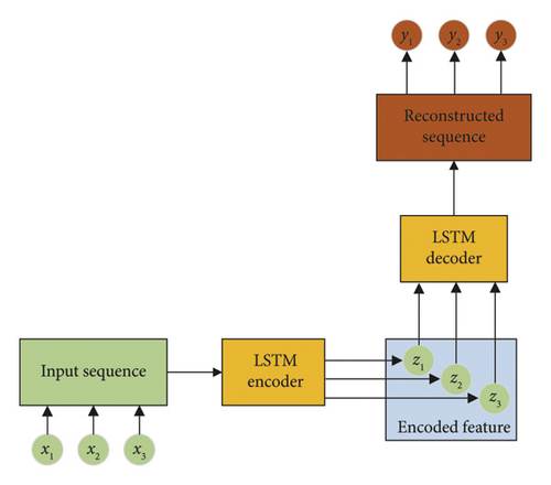
To solve the problem of LSTM network in processing time series data, an autoencoder and LSTM network are combined to obtain the reconstructed sequence of the original input sequence. Figure 2 represents the model diagram of an LSTM autoencoder. The main structure of the LSTM autoencoder consists of an encoder and a decoder, both using the LSTM network model. During the training process, they exclusively use normal electromagnetic samples with high confidence so that the model can only learn the deep semantic features of normal samples. During the training process, the autoencoder will conduct data reduction and compression of the original samples. This process discards irrelevant information, filters noise from the input data, and retains the main information in the sample. After the training, the new sample data are input into the LSTM autoencoder network and then fed into the fully connected layer for feature reconstruction. Afterward, the reconstructed value can be obtained, which is used to compare with the original input value.

Sometimes it is necessary to know the effect of an element in one position in the sequence on the whole time series. Dealing with this effectively using only LSTM can be challenging. Therefore, we employ the attention mechanism to solve this problem. The mapping relationship of the decoder for learning is expressed as h_θ : z⟶x. The output

of the decoder at the ith time can be expressed by the mapping function h_θ(⋅) as follows:

()

where z is the hidden layer variable, and

denotes the output of the decoder before the ith time. We can know that during the generation of

, the hidden layer variable z remains constant. The variable z is derived from the input sequence (x₁, x₂, …, x_n) through encoding, that is, the impact of different input values on the hidden variable remains constant, ensuring that each input value consistently contributes to the output value through calculations. In modeling time series data, it is evident that different input values have varying degrees of impact on the output values. At the same time, the length requirements of z vary depending on the task being processed. Therefore, the adaptive change of z can be achieved by using the attention mechanism. Also, we can obtain different encoded hidden variables z_i by adjusting the length of different input sequences, so the learning mapping relationship of the decoding layer can be expressed as

()

3.2.4. Construction of Sensing Statistics

In this paper, the proposed abnormal sensing model of LSTM autoencoder based on attention mechanism can reconstruct the input sample data. In the training process, only normal signal samples are used as the training set for the input network. This approach allows the neural network to learn solely the intrinsic features of the normal spectrum samples. During the sensing process, the network’s reconstruction effect on the abnormal input sample is significantly inferior to that of the normal sample. To assess the effectiveness of the reconstruction, we use the reconstruction error index for measurement purpose. Assume that the input sampled signal data is x = (x₁, x₂, …, x_n), the reconstructed output is y = (y₁, y₂, …, y_n), and we use the mean square error (MSE) as the reconstruction error function in this paper, which can be expressed as

()

In abnormal sensing problems, manually setting the threshold for sensing anomalies is a common method. However, this approach is susceptible to errors in judgment, especially when dealing with a large number of samples. So, we use the dynamic threshold division method to solve this problem [33]. Using the dynamic threshold

obtained by the dynamic threshold division method, when the reconstruction error is less than

, it indicates that the input sample signal is the normal sample. When the reconstruction error is greater than

, it indicates that the input sample signal is an abnormal sample. The whole decision process can be expressed by

()

where result = 0 denotes that the current sample is judged as a normal sample and result = 1 indicates that the current sample is judged as an abnormal sample. The procedure of the abnormal spectrum intelligent sensing using LSTM autoencoder based on attention mechanism with alpha-stable noise is summarized in Algorithm 1.

Algorithm 1: The abnormal spectrum intelligent sensing using LSTM autoencoder based on attention mechanism.

Require:x(k): the received signal.
Ensure: result: the abnormal spectrum judgment result.
1.
Suppress alpha-stable noise using DFN and use equations (10), (11), (17), and (19) to complete the feature extraction;
2.
Input the feaAs per style, Department is mandatory in affiliation. Please provide the Department/Division for affiliations 1, 2, 3, 5, and 7.ture sequence V of the normal sample into the autoencoder network to start network training. Map the input sequence V to the hidden space H through the feature mapping relation g_θ : x⟶z to complete the hidden feature learning of the input data;
3.
Adjust the length of different input sequences to encode different hidden variables z_i using the attention mechanism and use the mapping relationship to convert the hidden layer to the decoding layer;
4.
Determine whether the whole network has converged. If it has converged, save the network model M and proceed to Step 5. If not, proceed to Step 2;
5.
Denote the test sample sequence input to the network model M as P₁. After passing through the encoder network, the reconstructed sequence P₂ can be obtained, and the reconstruction error e between P₁ and P₂ can be calculated by equation (28);
6.
Use the dynamic threshold division method to obtain . If , the abnormal spectrum appears in the current monitoring spectrum; otherwise, it does not appear.

3.3. Abnormal Spectrum Intelligent Identification

3.3.1. Intelligent Characterization of Multifractal Spectrum Features

After sensing the abnormal spectrum using the collected signal samples, it is necessary to separate each abnormal spectrum sample using the identification algorithm so that the corresponding measures can be taken to deal with each abnormal spectrum according to its characteristics. This paper focuses on four kinds of abnormal spectrum signal types which have been extracted. We extract multifractal dimension spectrum features from them and then use these features as sample inputs to the deep forest model. Finally, we introduce the multigranularity scanning structure and cascade forest structure in the deep forest structure to enable the identification of several abnormal spectrum types.

First, the DFN is used to complete the suppression of alpha-stable noise in the sampled signal. Suppose that the characteristic sequence of a set of input abnormal spectrum is X = {x₁, x₂, …, x_k−1, x_k}, k = 1, 2.., N. For a feature sequence X, we divide it along one-dimensional coordinates using multiple one-dimensional boxes of size δ. If the sum of the sizes of all the feature sequence values divided by the ith box is S_i(δ), and the size of all the feature values of the sequence X is ∑S_i(δ), then the probability measure P_i(δ) represents the empirical probability of the average feature value size of the ith box and can be obtained as

()

Using the weight factor q, we can obtain the partition function χ_q(δ) by summing the q power exponents of probability measure P_i(δ). The calculation formula is expressed as

()

where q ∈ R and it is used to measure the unevenness of the multifractal object. When q > 1, the maximum value of P_i(δ) contributes least to χ_q(δ). In the scale-free interval, the relationship between the partition function and δ can be expressed as

()

Taking the logarithm of both sides, we can get the mass index function τ(q) as

()

If the obtained exponential function is linear, the fractal object is a single fractal object. If the obtained exponential function is a convex curve, the fractal object is a multifractal object. The multifractal spectrum index β and f(β) are calculated as

()

To calculate the multifractal spectrum, we concatenate the input feature sequence into the two-dimensional data matrix

, and the matrix dimension is M × N. After normalizing the matrix

, the magnitude matrix can be obtained by taking the absolute value, and a box of size δ is used to divide

. If the total mass of matrix

is Ω, we assume that the grid in row m and column n covers a matrix of mass m_i(δ), then the probability measure of the coverage matrix of the mn th grid can be obtained as

()

After obtaining P_i(δ), the partition function χ_q(δ) can be obtained by equation (31). Subsequently, the multifractal spectrum f(β) and the singularity exponent β can be obtained by equations (33) and (34). The four kinds of abnormal spectrum signals studied in this paper exhibit multifractal characteristics, and their multifractal spectrum function curves vary significantly. So, extracting the relevant feature parameters of the multifractal spectrum function can more accurately reflect the characteristics of different levels in various signals. To construct the feature vector set for abnormal spectrum identification, we calculate the maximum max(β) and minimum min(β) of the singular index in the multifractal spectrum function. In addition, we determine the singular index value β_m when the multifractal spectrum function reaches its maximum value, the fractal spectrum function values f₁ and f₂ corresponding to the maximum and minimum singular index, and the span Δf = f₁ − f₂ of the multifractal spectrum value in this paper. Then, we use these values to construct the input feature vector of the deep forest model

, which is expressed as

()

3.3.2. Deep Forest Model

Then, we use the deep forest model to identify the abnormal spectrum, which is explained in the following. Random forest is the primary component of the cascade deep forest, consisting of multiple subdecision trees. The decision tree compares the features of the input samples with the internal nodes through a layer-by-layer division process starting from the root node and progressing from top to bottom. This division process aims to classify the input samples into leaf nodes, each of which may contain multiple category labels. Suppose that the number of decision trees forming the random forest is C, the input sample set is E = [(a_i1, a_i2, …, a_id), b_i], i ∈ (1, L), L denotes the number of samples in the sample set, a_id represents the d th feature in the i th input sample, d is the total number of features in the sample, b_i stands for the label of the sample with b_i ∈ (1, M), and M represents the total number of categories.

An important step in the growth process of a decision tree is selecting classification features. The algorithm chooses the feature with the best performance from the multiclass features of the input sample set to split the current node. In this paper, we use the classification and regression tree (CART) algorithm to select features. In the CART algorithm, the Gini index is used as the standard for feature selection. The larger the value of the Gini index, the lower the purity of the currently divided data, so the feature with the smallest Gini index value is generally selected to divide the sample set. The expression of the Gini index is defined as

()

where p(i|S) denotes the proportion of samples with class label i in the total sample set E. Moreover, the Bagging method is used to select training samples in the process of random forest identification. For the input sample set S, Bagging extracts a subset of training samples from it, which are put back in size m each time. For some samples, it may be extracted several times, but some samples may never be selected. The samples that are not extracted for training can be referred to as out of bag (OOB). OOB data are typically chosen as the test set to evaluate the model’s generalization ability.

The primary part in the deep forest structure is the multigranularity scanning structure. In DNN, the enhancement of input samples’ features is typically achieved through convolution operations. The multigranularity scanning structure uses sliding window processing in convolution to transform the features of the initial input samples. This integration in breadth helps represent the interrelationship between different categories of samples, enabling a more accurate characterization of the sample. Suppose that the input feature data dimension is 1 × n, the sliding step of the introduced sliding window is 1, and the size of the window is 1 × m. Therefore, when performing feature scanning, a feature vector of size 1 × m will be calculated, and the size of the obtained sample feature dataset is (n − m + 1).

The process of multigranularity scanning can be expressed as follows. We assume that the input one-dimensional sample sequence is X = (x₁, x₂, …, x_n), the sliding window is W = (w₁, w₂, …, w_m) and m < n, and the sliding window step is k and (k < m), so we can obtain the scanned sequence set as N = (N₁, N₂, …, N_q), the sequence subset as N_q = (x_q, x_q+1, …, x_q+m−1) and q = 1, 2, …, (n − m)/k + 1. After multigranularity scanning of the input data, an n-dimensional sequence segment is expanded into (n − m + 1) new m-dimensional sequence segments to achieve data enhancement. The enhanced new sequence segments will be connected in parallel as the input feature vector Z for the subsequent cascade forest.

After enhancing the features using a multigranularity scanning structure, the next stage of the deep forest involves using a cascade structure to learn the features layer by layer. The input of each layer of the cascade forest consists of two parts, namely, the enhanced feature vector obtained after multigranularity scanning and the feature vector obtained after training the previous layer. To achieve a diverse data distribution, each layer of the cascade forest contains two types of structures, which are random forest and complete random forest. The difference between complete random forest and random forest is that the best-performing features are randomly selected from all input features for classification. Through this layer-by-layer training method, if the number of layers continues to increase and the identification performance is not significantly improved, the training process is terminated. This adaptive training method greatly reduces the impact of manual parameter adjustments on the robustness of identification.

In the defined cascade forest module, the first level of the cascade forest is denoted as ψ₁, and the input of the first level is defined as x so that the input vector of the second level of the cascade forest can be represented as [x, ψ₁(x)]. ψ₁(x) is the output vector of the first layer, and [a, b] stands for the process of forming a feature vector by connecting two feature vectors. We denote the feature tag set of the enhanced feature vector set Z as Y and extract a certain proportion of samples from Z as the training set S = ((z₁, y₁), (z₂, y₂), …, (z_n, y_n)), and they are all subject to the data distribution D. During the training process, the cascade forest learns the features of the input sample.

To describe the deep forest learning process, several characteristic modules in the deep forest learning process are explained in the following. The random forest module θ = (θ₁, θ₂, …, θ_d) is a submodule of the entire deep forest. The relationship for learning mapping in the random forest module of the dth layer of the cascade forest in the deep forest can be expressed as theta_d, and its specific process has been described above. The cascade forest module with multilayer connection U = (u₁, u₂, …, u_d) can be formed by several random forests and complete random forests, where u_d represents the dth layer of the cascade forest structure composed of random forests. Moreover, the output feature vector after passing through the cascade forest is ψ = (ψ₁, ψ₂, …, ψ_d), where ψ_d denotes the output feature vector of the dth layer of the cascade forest. The data distribution in each layer of the cascade forest can be expressed as D = (D₁, D₂, …, D_d).

For the learning mapping relationship θ_t of the random forest module in the tth cascade forest, its input includes the determined training set S and the output feature vector ψ_t(z_i), i ∈ [1, n] from the previous layer, where the data follow the distribution D_t, and A denotes the decision process of the random forest algorithm, which can be expressed as follows:

()

We use the defined random forest module to define the cascade forest module of d layers as follows:

()

The output feature vector of each layer of the cascade forest can be given by

()

where β_t denotes the system parameter, which requires constant adjustments during the training process to optimize the model. The procedure of the abnormal spectrum intelligent identification based on deep forest model with alpha-stable noise is summarized in Algorithm 2.

Algorithm 2: The abnormal spectrum intelligent identification based on the deep forest model.

Require:x(k): the received signal.
Ensure:type: the abnormal spectrum identification type.
1.
Suppress alpha-stable noise using DFNand use equations (10), (11), (17), and (19) to calculate feature sequences for several types of abnormal spectrum. Moreover, use equation (36) to calculate the multifractal spectrum characteristics of the feature sequences to obtain the input feature vector ;
2.
Extend the original input n dimensional sequence to (n − m + 1)m dimensional sequence segments with multigranularity scanning structure by using the method of scanning with sliding window and obtain the input feature vector of cascade forest by parallel connection;
3.
Input the feature vector into the random forest structure and the completely random forest structure of the first layer of the cascade forest, respectively. In the random forest, for the input i th sample, the kth decision tree will output M decision results p_i,k(b_i = c), c = (1, 2, …, M). Obtain the mean value of the output results of all subtrees in the forest to derive a class vector p_c;
4.
Connect the class vectors generated by all forests at each level of the cascade forest to the original inputs after multigranularity scanning to create enhanced features. These enhanced features will then serve as inputs for the next level. In the final layer, calculate the average of the class vectors produced by all the forests. Subsequently, determine the category that corresponds to the maximum mean value as the ultimate identification type;
5.
After extensive training, when the identification accuracy of the entire cascade forest no longer increases, the addition of more cascade layers is halted. This indicates that the entire identification process is complete.

4. Experimental Results and Analysis

To verify the effectiveness of the proposed method, we established an FM communication system in Matlab simulation platform to simulate and generate broadcast signals. In the simulation, the Simulink platform is used to simulate the medium wave AM broadcast system. The center frequency is 1000kHz and the bandwidth is 12kHz. In the abnormal spectrum sensing experiment, 30,000 samples of normal spectrum signals are collected as the training set required for network training. The signal point length of each signal sample is 1024 and the signal points in each sample are normalized. In the training process, the initial learning rate is 0.0001, the batch size per training is 256, the optimizer uses Adam, and the MSE is used to calculate the network loss. In addition, to illustrate the good performance of the proposed method, we use variational autoencoder (VAE), convolutional autoencoder (CAE), and traditional autoencoder (AE) to compare with the proposed method. In abnormal spectrum identification experiment, for several types of abnormal spectrum, 300 samples are collected under each GSNR as the training set and 200 samples are collected under each GSNR as the test set. The number of random forests in the cascade forest is set to 4 (two random forests and two completely random forests), the number of decision trees in a single random forest is set to 101, and the sliding window and step size in the multigranularity scan are set to 2 and 1, respectively.

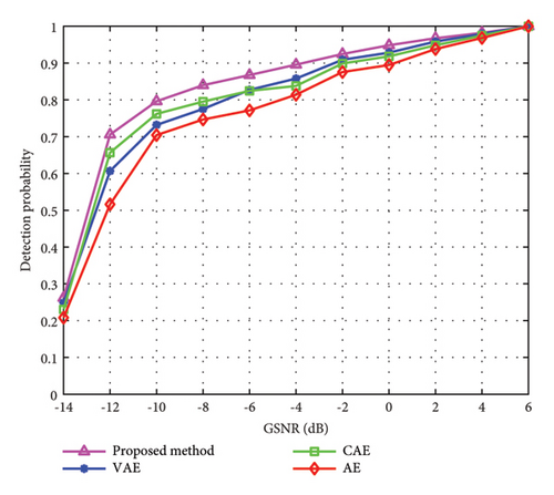
In addition to the receiver operating characteristic (ROC), we also use the area under the curve (AUC) as a parameter to measure the sensing performance of the model, and the AUC value represents the area under the ROC curve. Moreover, to measure the intensity of interference, we introduce the signal-to-interference ratio (SIR) for measurement, and it is expressed as

()

where P_s and P_n represent the power of the collected signal and the noise power, respectively.

In Figure 3, when SIR is 22 dB, we compare the abnormal spectrum sensing performance of the power exceeding standard of different methods under different GSNR. From Figure 3, it is observed that as the GSNR increases, the abnormal spectrum sensing probability of several methods gradually increases. When the GSNR is 2 dB, the abnormal spectrum sensing probability of the proposed method can reach 97.7%. Therefore, we can conclude that the proposed method outperforms existing methods in abnormal spectrum sensing performance for the power exceeding standard.

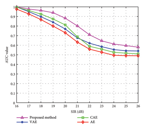
In Figure 4, when SIR is 20 dB, we compare the abnormal spectrum sensing performance of the power exceeding standard of different methods under different SIR. From Figure 4, we know that the proposed method can achieve an abnormal spectrum sensing accuracy of 87.1%. It can be found that when SIR is between 16 dB and 20 dB, the sensing effectiveness of CAE method is higher than that of VAE method. But with the gradual increase of SIR, the sensing performance of CAE method becomes lower than that of the VAE method. It can be seen from the comparison of the four curves that the proposed method has the best abnormal spectrum sensing performance within the specified SIR range when compared with existing methods.

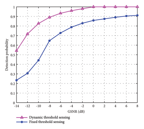
In Figure 5, we verify the influence of different threshold partitioning methods on the abnormal spectrum type sensing result of equipment failure under different GSNR. Moreover, we test the abnormal spectrum sensing performance of the dynamic threshold partitioning method and the fixed threshold partitioning method, respectively. As can be seen from Figure 5, with the continuous increase of GSNR, the sensing accuracy of the two threshold partitioning methods gradually increases. However, the fixed threshold partitioning method is difficult to adjust according to the reconstruction characteristics of different samples, so the overall sensing effectiveness of the fixed threshold partitioning method is significantly lower than that of the dynamic threshold partitioning method. When the GSNR is greater than -8 dB, the sensing accuracy of the dynamic threshold partitioning method is greater than 90%. Therefore, we can know that the dynamic threshold partitioning method has a more accurate sensing effect than the fixed threshold partitioning method, which proves the effectiveness of the proposed method.

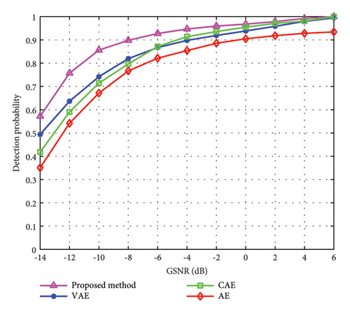
In Figure 6, we compare the abnormal spectrum sensing performance of frequency shift emission under different methods. From Figure 6, it can be seen that with the increase of GSNR, the abnormal spectrum sensing accuracy of several methods is constantly improving. Compared with other methods, the proposed method offers slightly higher sensing accuracy. When GSNR is -8 dB, the sensing accuracy of the proposed method can reach more than 90%. So, we can know that the proposed method has good abnormal spectrum sensing validity and is superior to existing methods.

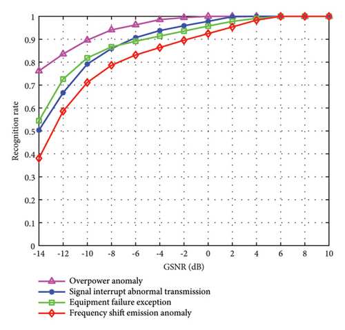
In Figure 7, we demonstrate the identification performance of the proposed method for different types of abnormal spectrum with different GSNR. From Figure 7, we can observe that as the GSNR continues to increase, the identification accuracy of several abnormal spectrum signals also rises. When the GSNR reaches -2 dB, the identification accuracy of all kinds of abnormal spectrum signals reach more than 90%. When the GSNR is 4 dB, the identification accuracy of all kinds of abnormal spectrum signals is close to 98%. For power exceeding standard, it is the easiest to identify. For signal interrupt transmission and equipment failure, the initial identification accuracy of the former is low. However, as the GSNR increases, the useful signals in the channel become more easily sensed, leading to a gradual improvement in the accuracy of identifying this anomaly. It can be seen that the proposed method is effective and feasible for several types of abnormal spectrum mentioned in this paper.

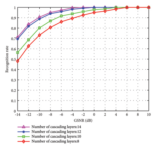
In Figure 8, we demonstrate the identification performance of the proposed method under different numbers of cascade layers with different GSNR. From Figure 8, it can be seen that as the number of cascade layers deepens, the overall identification accuracy shows an upward trend. This is because the deeper the cascade depth, the forest can acquire more enhanced features, enabling better learning of the samples. When the number of cascade layers increases to 12 and 14, the overall identification performance is very similar. This suggests that increasing the number of cascaded layers significantly improves identification accuracy. However, once the number of cascade layers exceeds a certain threshold, the identification accuracy will no longer increase.

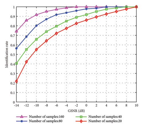
In Figure 9, to verify the impact of the number of training samples on the identification performance of the proposed method in this paper, the number of samples is set to 20, 40, 80, and 160, respectively. From Figure 9, it is seen that as the number of training samples and the GSNR increase, the identification rate of the proposed method continues to rise. When the number of training samples is 20 and the GSNR is 2 dB, the rate can only reach less than 90%. When the number of samples is 160 and the GSNR is -6 dB, the identification rate can reach over 95%. Therefore, we can know that the identification performance of the proposed method can be significantly enhanced by using a large number of samples properly during training.

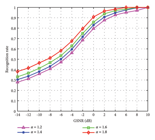
In Figure 10, we demonstrate the identification performance of the proposed method under different characteristic exponents α with different GSNR. From Figure 10, we can observe that as the characteristic exponent increases continuously, the identification performance shows an upward trend. When α = 1.2 and α = 1.4, the identification performances are very close. When α = 1.8, the identification accuracy reaches its maximum. In addition, when α = 1.8 and the GSNR is 0 dB, the identification accuracy of the proposed method can reach more than 90%. So, we can know that setting the value of the characteristic exponent α to a larger value enhances the identification performance of the proposed method.

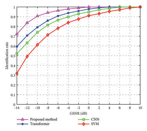
In Figure 11, we compare the abnormal spectrum identification performance between the proposed method and existing methods under different GSNR. From Figure 11, it is shown that the identification rate of the proposed method is significantly better than that of existing methods. With the continuous increase of the GSNR, the identification rate of all methods is rising. When the GSNR reaches −10 dB, the identification rate of the proposed method can reach 90%, while other methods are lower than 80%, indicating that the proposed method has good abnormal spectrum identification performance.

5. Conclusion

This paper proposes the abnormal spectrum intelligent sensing and identification method with alpha-stable noise. First, we suppress alpha-stable noise using the DFN. Then, we propose an attention-mechanism-based LSTM autoencoder method to sense abnormal spectrum. Moreover, in the sensing process, the reconstruction error between the normal sample signal and the abnormal sample signal is used as the sensing statistic, and the sensing threshold is determined by a dynamic threshold division method. Next, we propose a method to identify the abnormal spectrum based on a deep forest model. We extract the multifractal spectrum features from several abnormal spectrum representation sequences and enhance the original input features by using the multigranularity scanning structure. In addition, the class vector generated by all forests is averaged and then the final identification type is determined by maximizing the mean class. The experimental results show that the proposed method is better than existing methods in abnormal spectrum sensing and identification. In abnormal spectrum sensing, the proposed method demonstrates more stable performance compared with existing methods. In abnormal spectrum identification, the proposed method exhibits strong parameter robustness.

Moreover, the integration of satellite and terrestrial networks has a wide coverage area and good communication capability. However, the number of nodes in the network is large, the distance between each other is long, the distribution is irregular, and a large number of spectrum sensing data will make the transmission link become crowded, resulting in unpredictable errors. In addition, the link of the integration of satellite and terrestrial networks changes rapidly, and the spectrum sensing results are not timely, and so on. All these bring challenges to the spectrum sensing discussed in this paper. Therefore, in the future, we will study the challenges posed by the integration of satellite and terrestrial networks to spectrum sensing and optimize the shortcomings of RNN variants such as GRU and bidirectional LSTM so as to better complete the tasks mentioned in this paper.

Conflicts of Interest

The authors declare no conflicts of interest.

Funding

This work was supported by the National Natural Science Foundation of China under Grants U2441250, 62231027, and 62301380, in part by the Natural Science Basic Research Program of Shaanxi under Grant 2024JC-JCQN-63, in part by the China Postdoctoral Science Foundation under Grant 2022M722504, in part by the Postdoctoral Science Foundation of Shaanxi Province under Grant 2023BSHEDZZ169, in part by the Key Research and Development Program of Shaanxi under Grant 2023-YBGY-249, and in part by the Guangxi Key Research and Development Program under Grant 2022AB46002.

Acknowledgments

Open Research

Data Availability Statement

No data were used to support the findings of this study.

References

1 Shen J., Zhou T., He D., Zhang Y., Sun X., and Xiang Y., Block Design-Based Key Agreement for Group Data Sharing in Cloud Computing, IEEE Transactions on Dependable and Secure Computing. (2019) 16, no. 6, 996–1010, https://doi.org/10.1109/tdsc.2017.2725953, 2-s2.0-85023594994.
10.1109/TDSC.2017.2725953
Web of Science® Google Scholar
2 Lee K., Comments on “Secure Data Sharing in Cloud Computing Using Revocable-Storage Identity-Based Encryption, IEEE Trans. Cloud Comput. (2020) 8, no. 4, 1299–1300, https://doi.org/10.1109/tcc.2020.2973623.
10.1109/TCC.2020.2973623
Web of Science® Google Scholar
3 Zeng W. and Koutny M., Quantitative Analysis of Opacity in Cloud Computing Systems, IEEE Trans. Cloud Comput.(2021) 9, no. 3, 1210–1219, https://doi.org/10.1109/tcc.2019.2894768, 2-s2.0-85060432277.
10.1109/TCC.2019.2894768
Web of Science® Google Scholar
4 Ardagna D., Panicucci B., and Passacantando M., Generalized Nash Equilibria for the Service Provisioning Problem in Cloud Systems, IEEE Trans. Serv. Comput.(2013) 6, no. 4, 429–442, https://doi.org/10.1109/tsc.2012.14, 2-s2.0-84890482773.
10.1109/TSC.2012.14
Web of Science® Google Scholar
5 Mei J., Li K., Tong Z., Li Q., and Li K., Profit Maximization for Cloud Brokers in Cloud Computing, IEEE Transactions on Parallel and Distributed Systems. (2019) 30, no. 1, 190–203, https://doi.org/10.1109/tpds.2018.2851246, 2-s2.0-85049153285.
10.1109/TPDS.2018.2851246
Web of Science® Google Scholar
6 Liu M., Mao Y., and Leng S., Cooperative Fog-Cloud Computing Enhanced by Full-Duplex Communications, IEEE Communications Letters. (2018) 22, no. 10, 2044–2047, https://doi.org/10.1109/lcomm.2018.2866145, 2-s2.0-85052699777.
10.1109/LCOMM.2018.2866145
Web of Science® Google Scholar
7 Lee C. and Fumagalli A., Internet of Things Security: Multilayered Method for End to End Data Communications over Cellular Networks, Proc. IEEE 5th World Forum Internet Things (WF-IoT), April 2019, 24–28.
Google Scholar
8 Liu Y., Wang K., Qian K., Du M., and Guo S., Tornado: Enabling Blockchain in Heterogeneous Internet of Things Through a Space-Structured Approach, IEEE Internet of Things Journal. (2020) 7, no. 2, 1273–1286, https://doi.org/10.1109/jiot.2019.2954128.
10.1109/JIOT.2019.2954128
Web of Science® Google Scholar
9 Ismael W. M., Gao M., Zahary A., Yemeni Z., Ibrahim Y., and Hawban A., Edge-based Anomaly Data Detection Approach for Wireless Sensor Network-Based Internet of Things, Proceedings International Conference on Information Technology, March 2021, Sci. Adm. (ICTSA), 1–6.
Google Scholar
10 Yu R., Zhang X., and Zhang M., Smart Home Security Analysis System Based on the Internet of Things, Proc. IEEE 2nd Int. Conf. Big Data, Artif. Intell. Internet Things Eng. (ICBAIE), March 2021, 596–599, https://doi.org/10.1109/icbaie52039.2021.9389849.
10.1109/icbaie52039.2021.9389849
Google Scholar
11 Atzori L., Campolo C., Da B. et al., Enhancing Identifier/Locator Splitting through Social Internet of Things, IEEE Internet of Things Journal. (2019) 6, no. 2, 2974–2985, https://doi.org/10.1109/jiot.2018.2877756, 2-s2.0-85055714494.
10.1109/JIOT.2018.2877756
Web of Science® Google Scholar
12 López-Benítez M., Majumdar C., and Merchant S. N., Aggregated Traffic Models for Real-World Data in the Internet of Things, IEEE Wireless Commun. Lett.(2020) 9, no. 7, 1–1050, https://doi.org/10.1109/lwc.2020.2980272.
10.1109/LWC.2020.2980272
Web of Science® Google Scholar
13 Li W., Song H., and Zeng F., Policy-Based Secure and Trustworthy Sensing for Internet of Things in Smart Cities, IEEE Internet of Things Journal. (2018) 5, no. 2, 716–723, https://doi.org/10.1109/jiot.2017.2720635, 2-s2.0-85023758110.
10.1109/JIOT.2017.2720635
Web of Science® Google Scholar
14 Kurniawan B., Supangkat S., Lumban Gaol F., and Ranti B., Framework for Developing Smart City Models in Indonesian Cities (Based on Garuda Smart City Framework), Proc. Int. Conf. ICT Smart Soc. (ICISS), August 2022, 1–5.
Google Scholar
15 Ma C., Vu H. Q., Wang J., Trieu V.-H., and Li G., Understanding Residents’ Behavior for Smart City Management by Sequential and Periodic Pattern Mining, IEEE Transactions on Computational Social Systems. (2024) 11, no. 1, 1260–1276, https://doi.org/10.1109/tcss.2023.3249740.
10.1109/TCSS.2023.3249740
Web of Science® Google Scholar
16 Li X., Jing T., Wang X., Han D., Fan X., Dong H., Li X., and Richard Yu F., Two-Stage Offloading for an Enhancing Distributed Vehicular Edge Computing and Networks: Model and Algorithm, IEEE Transactions on Intelligent Transportation Systems. (2024) 25, no. 11, 17744–17761, https://doi.org/10.1109/TITS.2024.3424852.
10.1109/TITS.2024.3424852
Web of Science® Google Scholar
17 Liu M., Zhang Z., Chen Y., Ge J., and Zhao N., Adversarial Attack and Defense on Deep Learning for Air Transportation Communication Jamming, IEEE Transactions on Intelligent Transportation Systems. (2024) 25, no. 1, 973–986, https://doi.org/10.1109/tits.2023.3262347.
10.1109/TITS.2023.3262347
CAS Web of Science® Google Scholar
18 Zhu E., Zhou Z., Ma Z., Li X., and Liu F., Secure and Efficient Collaborative Auction Scheme for Spectrum Resource Reallocation, Proc. IEEE 22nd Int. Conf. Comput. Supported Cooperative Work Des. ((CSCWD)), May 2018, 396–400, https://doi.org/10.1109/cscwd.2018.8465154, 2-s2.0-85054409189.
10.1109/cscwd.2018.8465154
Google Scholar
19 Fan Y., Su T., and Chen Z., Wireless Emergency Communication Method Based on Electromagnetic Spectrum Environment Sensing, Proc. IEEE 6th Int. Conf. Pattern Recognit. Artif. Intell. (PRAI), August 2023, 1142–1146, https://doi.org/10.1109/prai59366.2023.10331954.
10.1109/prai59366.2023.10331954
Google Scholar
20 Wang Q., Sun Q., Ren K., and Jia X., THEMIS: Collusion-Resistant and Fair Pricing Spectrum Auction under Dynamic Supply, IEEE Transactions on Mobile Computing. (2017) 16, no. 7, 2051–2064, https://doi.org/10.1109/tmc.2016.2609425, 2-s2.0-85027502839.
10.1109/TMC.2016.2609425
CAS Web of Science® Google Scholar
21 Wang Q., Ye B., Xu T., Lu S., and Guo S., DOTA: A Double Truthful Auction for Spectrum Allocation in Dynamic Spectrum Access, Proc. IEEE Wireless Commun. Networking Conf. (WCNC), April 2012, 1490–1495, https://doi.org/10.1109/wcnc.2012.6214017, 2-s2.0-84864374146.
10.1109/wcnc.2012.6214017
Google Scholar
22 Wang B., Yuan Z., Lu J., and Zhang X., Multitask Collaborative Learning Neural Network for Radio Signal Classification, IEEE Transactions on Communications. (2024) https://doi.org/10.1109/TCOMM.2024.3477322.
10.1109/TCOMM.2024.3477322
Google Scholar
23 Li L., Application Analysis of Radio Interference Signal Network Monitoring and Positioning Technology, Digital Commun. World. (2022) 212, no. 8, 111–113.
Google Scholar
24 Wang H., Analysis of Radio Interference Signal Detection and Recognition, China New Telecommun.(February 2021) 23, no. 3, 3–4.
Google Scholar
25 Gao X., Analysis of Radio Interference and Radio Management Countermeasures, Digital Commun. World. (2020) 187, no. 7.
Google Scholar
26 Rajendran S., Meert W., Lenders V., and Pollin S., Unsupervised Wireless Spectrum Anomaly Detection with Interpretable Features, IEEE Transactions on Cognitive Communications and Networking. (2019) 5, no. 3, 637–647, https://doi.org/10.1109/tccn.2019.2911524, 2-s2.0-85064599791.
10.1109/TCCN.2019.2911524
Web of Science® Google Scholar
27 Zhou X., Xiong J., Zhang X., Liu X., and Wei J., A Radio Anomaly Detection Algorithm Based on Modified Generative Adversarial Network, IEEE Wireless Commun. Lett.(2021) 10, no. 7, 1552–1556, https://doi.org/10.1109/lwc.2021.3074135.
10.1109/LWC.2021.3074135
Web of Science® Google Scholar
28 Wang X. Y., Yang J. J., Zhang L., Lu Q. N., and Huang M., Spectrum Monitoring of Radio Digital Video Broadcasting Based on an Improved Generative Adversarial Network, Radio Science. (2021) 56, no. 8, 1–13, https://doi.org/10.1029/2021rs007270.
10.1029/2021RS007270
Web of Science® Google Scholar
29 Wang G.-S., Ren Q.-H., and Su Y.-Z., The Interference Classification and Recognition Based on SF-SVM Algorithm, 2017 IEEE 9th International Conference on Communication Software and Networks (ICCSN), May 2017, 835–841, https://doi.org/10.1109/iccsn.2017.8230229, 2-s2.0-85049192977.
10.1109/iccsn.2017.8230229
Google Scholar
30 Chen X., He D., Yan X., Yu W., and Truong T.-K., GNSS Interference Type Recognition with Fingerprint Spectrum DNN Method, IEEE Transactions on Aerospace and Electronic Systems. (2022) 58, no. 5, 4745–4760, https://doi.org/10.1109/taes.2022.3167985.
10.1109/TAES.2022.3167985
Web of Science® Google Scholar
31 Wang P., Cheng Y., Shang G., Wang J., and Li S., Time-Frequency Component-Aware Convolutional Neural Network for Wireless Interference Classification, IEEE Wireless Commun. Lett.(2022) 11, no. 12, 2487–2491, https://doi.org/10.1109/lwc.2022.3204756.
10.1109/LWC.2022.3204756
Web of Science® Google Scholar
32 Ke Z. and Vikalo H., Real-Time Radio Technology and Modulation Classification via an LSTM Auto-Encoder, IEEE Transactions on Wireless Communications. (2022) 21, no. 1, 370–382, https://doi.org/10.1109/twc.2021.3095855.
10.1109/TWC.2021.3095855
Web of Science® Google Scholar
33 Hundman K., Constantinou V., Laporte C., Colwell I., and Soderstrom T., Detecting Spacecraft Anomalies Using LSTMs and Nonparametric Dynamic Thresholding, in Proceedings of the 24th ACM SIGKDD International Conference on Knowledge Discovery & Data Mining, August 2018, 387–395, https://doi.org/10.1145/3219819.3219845, 2-s2.0-85051518933.
10.1145/3219819.3219845
Google Scholar

All articles

Intelligent Sensing and Identification of Spectrum Anomalies With Alpha-Stable Noise

Abstract

1. Introduction