SCA-Net: Seasonal Cycle-Aware Model Emphasizing Global and Local Features for Time Series Forecasting
Abstract
Recent advances in transformer architectures have significantly improved performance in time-series forecasting. Despite the excellent performance of attention mechanisms in global modeling, they often overlook local correlations between seasonal cycles. Drawing on the idea of trend-seasonality decomposition, we design a seasonal cycle-aware time-series forecasting model (SCA-Net). This model uses a dual-branch extraction architecture to decompose time series into seasonal and trend components, modeling them based on their intrinsic features, thereby improving prediction accuracy and model interpretability. We propose a method combining global modeling and local feature extraction within seasonal cycles to capture the global view and explore latent features. Specifically, we introduce a frequency-domain attention mechanism for global modeling and use multiscale dilated convolution to capture local correlations within each cycle, ensuring more comprehensive and accurate feature extraction. For simpler trend components, we apply a regression method and merge the output with the seasonal components via residual connections. To improve seasonal cycle identification, we design an adaptive decomposition method that extracts trend components layer by layer, enabling better decomposition and more useful information extraction. Extensive experiments on eight classic datasets show that SCA-Net achieves a performance improvement of 12.1% in multivariate forecasting and 15.6% in univariate forecasting compared to the baseline.
1. Introduction
Time-series forecasting aims to leverage past observations to model and capture underlying patterns such as trends, seasonality, and other data behaviors, which are essential for making future predictions. This task is crucial in various fields, including finance [1, 2], weather [3, 4], transportation [5, 6], and energy [7], where it supports decision-making, resource allocation, and efficiency optimization. The complexity of time-series forecasting grows with the length of the prediction horizon, which is commonly divided into short-term [8], medium-term [9], and long-term [10–12] categories, each presenting unique challenges. This paper aims to delve into the challenges of long-sequence forecasting tasks, exploring the methods and techniques necessary for addressing more demanding prediction problems. Here, we focus on the dynamic changes in data over extended periods, aiming to enhance the accurate prediction of future trends in the face of more complex and longer-term application scenarios.
Time-series forecasting methods have evolved from classical statistical techniques, such as autoregressive integrated moving average (ARIMA) [13] and exponential smoothing [14], to machine learning approaches, including support vector machine [15], decision tree [16], and random forest models [17]. Recently, deep learning methods [18] have demonstrated remarkable potential in this field, particularly with models such as recurrent neural networks (RNNs) [19], convolutional neural networks (CNNs) [20], and transformers [21]. These advancements provide more powerful and flexible tools for time-series forecasting. Moreover, this evolution reflects the ongoing pursuit of handling complex, nonlinear temporal relationships, rendering deep learning methods widely applied and high-performing techniques in current time-series forecasting.
The RNN is a neural network architecture specifically designed to handle sequential data, introducing recurrent units that allow the network to maintain a form of memory mechanism to process input information at different time steps. Typically, an RNN comprises one or more recurrent units, where each unit receives input from the current time step and the hidden state from the previous time step, producing the current time step output along with a new hidden state. RNNs exhibit flexibility in handling sequential data, effectively capturing time-dependent relationships across sequences of varying lengths. However, RNNs can suffer from problems, such as vanishing and exploding gradients [22], particularly evident when dealing with long sequences, limiting their ability to effectively model long-term dependencies. Moreover, RNN computations are usually performed sequentially, making parallelization challenging and resulting in lower efficiency when dealing with large-scale data. To overcome these limitations, improved models based on RNNs have been proposed, such as the long short–term memory (LSTM) [23] and gated recurrent unit (GRU) [24] models, enhancing their ability to effectively model long-term dependencies. The LSTM introduces forget, input, and output gates to better capture and process long-term dependencies. However, it comes with higher computational costs and more parameters, making it prone to overfitting. By contrast, the GRU features a relatively simplified structure with lower computational costs and fewer parameters, making it more suitable for scenarios where computational efficiency is crucial; however, it may not perform as well as the LSTM in capturing long-term dependencies.
The CNN is a deep learning model that has gained significant success in computer vision (CV) tasks [25–27] and, in recent years, has been effectively adapted for time-series forecasting [28]. In time-series applications, CNNs excel at identifying local patterns and correlations, making them effective for problems with clear temporal locality, such as short-term trends and periodic variations. However, CNNs struggle with capturing long-range dependencies in time-series data. To address this, the temporal convolutional network (TCN) [29] was developed. By incorporating techniques such as dilated convolution [30] and residual connections [31], the TCN expands the receptive field and enhances the CNN’s ability to model long-term dependencies. Residual connections help alleviate the vanishing gradient problem, ensuring stable training even with deeper networks.
The transformer has become a dominant architecture in modern deep learning applications. Motivated by its proven effectiveness in NLP [32] and CV [33, 34], the method is increasingly applied to time-series forecasting, particularly for capturing temporal patterns over long horizons. Nonetheless, the self-attention mechanism it relies on [35, 36] incurs a considerable computational burden [37], especially as input lengths increase, which constrains its scalability in practical environments. While the transformer excels at capturing global interactions within a sequence, such exhaustive modeling may not always be ideal for temporal data that follows cyclical or seasonal trends. In such cases, repeated patterns within individual cycles often play a more pivotal role than distant dependencies.
Moreover, regardless of domain differences, time-series data commonly demonstrate features such as trends and seasonal regularity. Trend-seasonality decomposition methods [38] help uncover the underlying structure of time-series data, thereby facilitating more accurate predictions. Trend-seasonality decomposition breaks down a time series into a combination of multiple periodic and nonperiodic components, that is, seasonal and trend components. By modeling these two components, a better understanding can be obtained regarding the long-term trends and periodic patterns in the time series. The decomposition process is akin to smoothing the time series, reducing the impact of random noise. By examining both trend evolution and recurring seasonal behaviors, one can uncover underlying structures within temporal datasets, thereby facilitating more precise forecasting and deeper analytical insights. Moreover, different seasonal cycles within a time series exhibit unique local features. For example, in Figure 1, seasonal cycle charts at different time scales are plotted, revealing distinct data patterns within a day compared to patterns within a week or a month. It is evident that local correlations between these different seasonal cycles exist, showing variations and relationships at different time scales. To better understand the time-series dynamics and to gain greater insight into the features and trends present in time-series data, it is crucial to extract and analyze the local correlations among these seasonal cycles, uncovering their changes and interrelationships across various time scales.
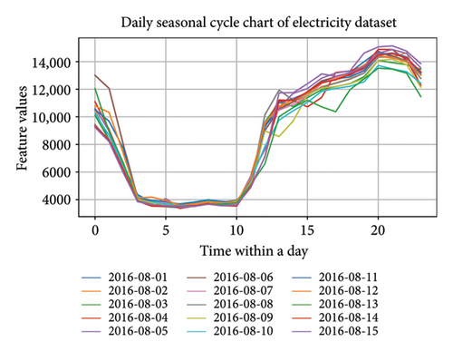
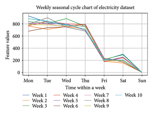
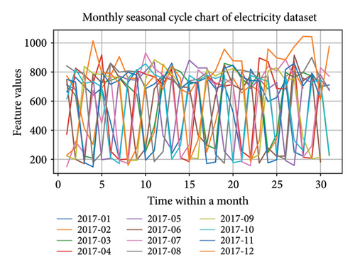
Consequently, this study presented a layered extraction method for seasonal and trend components of time-series data using a trend-seasonality decomposition method that was adaptive to the seasonal cycle. A dual-branch design was adopted to extract seasonal and trend information individually, in accordance with their inherent structures. For the seasonal components containing complex features, a combination of global and local feature extraction was applied. The time series was globally analyzed in the frequency domain for feature extraction, followed by extracting features for each seasonal cycle in the time domain. Frequency domain parity correction attention (FPCA) [39] was utilized to globally model the seasonal components, and multiscale dilated convolution [39] was leveraged to extract local features within each seasonal cycle. Through an integrated approach in both the frequency and time domains, coordinating global and local characteristics, more comprehensive and richer seasonal cycle features could be extracted. For trend components with relatively simple feature components, a straightforward regression method was used to obtain more accurate trend components. Finally, combining the seasonal and trend features yielded accurate time-series feature components for the definitive sequence prediction. Consequently, a seasonal cycle-adaptive trend-seasonality decomposition (SCASeriesDecomp) module was introduced to address the limitations of existing trend-seasonality decomposition methods in obtaining more precise seasonal cycle components. This model calculated the accurate seasonal cycle components in time-series data, separating the time series into seasonal and trend components. This paper conducted extensive experiments on the aforementioned basic framework based on the two mainstream embedding approaches: Channel independent (CI) and channel mixed (CM). The experimental results not only validate the effectiveness of the framework but also demonstrate that the model achieves significant performance improvements compared to classic models under both embedding strategies. This indicates that the model exhibits strong adaptability and stability across different embedding strategies.
- •
We presented a novel time-series forecasting model (seasonal cycle-aware time-series forecasting model [SCA-Net]), which employed a dual-branch feature extraction architecture for the separate extraction of features related to seasonal and trend components.
- •
We introduced a seasonal forecasting block (SFB) that combined frequency and time domain methods, jointly extracting the global and local features of seasonal cycles. This module employs a specially designed attention mechanism in the frequency domain, which leverages odd–even signal separation and feature refinement techniques, serving as a replacement for self-attention and cross-attention mechanisms in modeling long-range periodic dependencies. In addition, it incorporated a multiscale dilated convolution to extract features within each seasonal cycle, resulting in the accurate representation of seasonal patterns.
- •
We introduced a SCASeriesDecomp method, which accurately identified seasonal cycle patterns in time-series data. This method enabled the precise separation of trend components, facilitating the layered extraction of the accurate seasonal and trend components for subsequent modeling.
- •
We conducted extensive experiments on eight datasets, and the results demonstrated that our method achieves excellent forecasting performance in both multivariate and univariate predictions. Specifically, in multivariate prediction, we validated both the CM and CI embedding approaches, proving that the model can effectively enhance forecasting performance compared to classic models based on these embedding strategies.
2. Related Work
2.1. Time-Domain and Frequency-Domain Modeling
Traditional time-series models typically operate directly in the time domain, focusing on the original data to capture instantaneous changes, which is essential for identifying abrupt shifts, short-term trends, or periodic patterns. For example, Informer [40] reduces computational complexity through the ProbSparse self-attention mechanism and improves long-sequence forecasting efficiency by incorporating a distillation method [41–43] to compress sequence length. Pyraformer [44] employs a tree structure with pyramid attention to extract features at different resolutions in the time domain. The MTPNet [45] proposes a multiscale transformer pyramid network that combines dimension-invariant embedding with multiscale modeling to capture temporal dependencies at varying granularities. Crossformer [46] introduces cross-dimensional correlations and a two-stage attention mechanism (TSA) for capturing dependencies across both time and dimensions. However, the use of CM embeddings in many time-series models often limits the ability to capture temporal dependencies, as they focus on channel interactions rather than temporal evolution. The CI embedding strategy addresses this by enabling independent processing of each channel while maintaining temporal correlations. PatchTST [47] enhances this by combining CI embedding with patching methods, treating each channel of a multivariate series as an independent univariate time series. This improves memory efficiency and allows the model to handle longer sequences, enhancing long-term forecast accuracy. Despite these advancements, time-domain models still struggle with capturing long-term dependencies and global features, especially in long sequences.
The Autoformer [48] introduces an autocorrelation mechanism based on the Wiener–Khinchin theorem and applies Fourier transforms to uncover periodic dependencies. This frequency-domain approach, applied in the FEDformer [49], uses frequency-enhanced blocks (FEBs) for attention mechanisms, which improves global feature extraction and captures periodic trends. The FiLM [50] uses Fourier analysis combined with low-rank approximation and Legendre projection to address issues such as noise and overfitting, offering deeper insight into the global characteristics of time-series data. However, frequency-domain methods often struggle with short-term fluctuations and local changes.
To leverage the strengths of both domains, a hybrid approach combines frequency-domain modeling for global features with time-domain modeling to capture local seasonal cycles. This integration of global and local information offers a more comprehensive view of time-series dynamics, improving model robustness and adaptability across varying scales and frequencies. The combined approach provides a more effective modeling strategy for time-series forecasting.
2.2. Fourier Component Selection
In the Fourier transform, f represents the frequency, and j denotes the imaginary unit. It decomposes a signal into spectral components, offering insight into the signal’s frequency content. Low-frequency components correspond to slow variations or long-term trends in the time series, while high-frequency components capture rapid fluctuations and short-term changes. In the FEDformer, the time series is transformed into the frequency domain, but retaining all frequency components can lead to overfitting and excessive noise, negatively impacting predictive performance. To mitigate this, a method of randomly selecting a subset of Fourier components is used, which retains both high- and low-frequency components. This improves the model’s effectiveness, though random selection may omit important frequency components, which can degrade prediction accuracy.
Similarly, the FiLM method selects a subset of frequency components, choosing the lowest M to reduce noise and training time. However, incorporating some high-frequency components can improve performance, highlighting that omitting certain frequency components risks losing important features, ultimately affecting predictions.
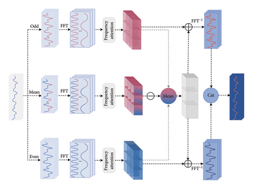
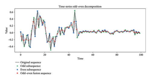
To address these issues, we propose a strategy that splits the time series into odd- and even-indexed segments, modeled separately in the frequency domain. This approach alleviates overfitting and reduces high-frequency noise, which commonly arises when keeping all Fourier components. In addition, it eliminates the uncertainty introduced by random selection of components [51, 52] and avoids the loss of information linked to focusing only on low-frequency components. Odd–even decomposition, a form of downsampling, preserves the overall structure and key features of the time series, enhancing the model’s ability to focus on the essential patterns while minimizing attention to noise. Since noise tends to be uniformly distributed across the odd and even components, separating these components helps mitigate the noise’s effect on the observed trends and cycles. This separation also improves the accuracy of frequency-domain feature extraction. However, downsampling in odd–even decomposition can result in the loss of high-frequency details, which could affect the model’s ability to capture fast-changing features. To address this, we introduce an odd–even fusion term, combining the benefits of odd–even decomposition while compensating for any lost information, thereby enhancing the model’s robustness.
The inverse Fourier transform, calculated as described above, reassembles the frequency spectrum components in the original time-domain signal.
2.3. Trend-Seasonality Decomposition
Trend-seasonality decomposition is a commonly used method in time-series analysis, forecasting, and modeling. It involves separating a sequence into its trend, seasonal, and residual components, providing a deeper understanding of the sequence’s behavior and fluctuations. By breaking down time-series data, the structure of the sequence becomes more apparent, supporting the development of more precise predictive models. Seasonal components capture recurring patterns within fixed intervals, while the goal of seasonal decomposition is to extract these periodic variations. Trend components represent the long-term changes in the data, and trend decomposition focuses on isolating these long-term patterns to better capture the sequence’s overall evolution.
However, these three methods have a significant drawback: they require continuous adjustments to the pooling window size. Since the choice of pooling window size directly affects the ability to capture seasonal changes, in practical applications, it can be challenging to determine an appropriate window size in advance. Consequently, it cannot be guaranteed that a highly accurate seasonal periodicity of the time series will be found. To address this problem, we presented a SCASeriesDecomp strategy, using a Fourier transform to discover the primary cycles in the time series as pooling windows. By employing this method, we can accurately capture seasonal patterns at different scales and variations, reducing dependence on the manual adjustment of hyperparameters.
2.4. Encoder–Decoder
In this approach, we eliminate the traditional encoder stack and rely on a single-layer decoder to jointly perform both encoding and decoding functions. This technique enables both the extraction of time-series characteristics and the forecasting of future data points. We introduce a one-step generative decoder architecture, which removes the need for an encoder and utilizes a single layer for generating predictions. Unlike the generative decoder in the Informer, this decoder can sample the full input sequence as Ltoken, incorporating both the sequence length for predictions and the input data during training. By handling information modeling in a unified manner, it can compute all forecasted values in one forward pass, significantly enhancing the model’s efficiency in both space and time. Experimental results show that this one-layer generative decoder can still deliver outstanding forecasting performance.
3. Methodology
3.1. Preliminary
Time-series forecasting leverages historical data to predict upcoming observations. This task can be formulated as a mapping function f, such that Y = f(X). In this context, the input sequence X = [X1, X2, …, Xt, …, XT] represents historical data points, where Xt is the observed value at time t and T is the total sequence length. The target sequence is expressed as Y = [Y1+h, Y2+h, …, Yt+h, …, YT+h], with Yt+h representing the forecasted value at time t + h, and h indicating the prediction horizon.
3.2. Overall Architecture
This paper introduces a dual-branch model framework based on seasonal cycle awareness. To verify the effectiveness of this framework, we applied it to two mainstream embedding methods: CI and CM, and conducted model predictions. Subsequently, we compared the prediction results with existing classic models based on CI and CM, providing a comprehensive evaluation of our framework’s advantages under different embedding strategies. This comprehensive evaluation confirms that the proposed framework is capable of retaining essential features within time-series data, while also showcasing enhanced performance in modeling interactions across different channels. It presents a well-balanced approach for addressing multivariate time-series forecasting tasks.
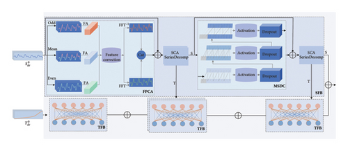
The proposed model utilizes a decomposition technique to separate the time series into seasonal and trend components, employing a dual-branch feature extraction framework to handle each component independently. Unlike the Autoformer and FEDformer models, where the trend-seasonality decomposition struggles to identify a precise seasonal cycle, we introduce a seasonal cycle-adaptive decomposition model that gradually breaks the time series into its seasonal and trend parts. Consequently, the previous approach of modeling only the seasonal component in Autoformer and FEDformer is abandoned. In response, we develop a parallel architecture that separately predicts periodic and trend-related patterns, leveraging their unique temporal characteristics. The final forecast is obtained by combining predictions from both components.
For capturing complex seasonal patterns, we incorporate a SFB for feature extraction. Instead of relying on conventional self- and cross-attention mechanisms, this block uses a frequency-based attention method called parity correction attention. Together with multiscale dilated convolutions, this enables efficient global information modeling in the frequency domain while enhancing local feature extraction in the time domain, thereby improving the model’s ability to learn latent patterns in the time series. To process the trend component, we use a trend-cyclical forecasting block (TFB), which extracts trend-related features via a simple fully connected layer. This block identifies internal correlations, uncovering hidden relationships in the data to better understand the trend behavior. As shown in Figure 2, the “odd” and “even” components represent the odd and even parts from the time-series decomposition, while “mean” refers to the fused odd–even component. “FA” indicates the frequency-domain attention mechanism, and “S” and “T” represent the seasonal and trend components, respectively.
The proposed model comprises two blocks, that is, the SFB and the TFB. The SFB includes the SCASeriesDecomp, FPCA, multiscale dilated convolutional (MSDC), and three main blocks. The detailed descriptions of the SCASeriesDecomp, FPCA, MSDC, and TFB are provided in Sections 3.3.1, 3.3.2, 3.3.3, and 3.4, respectively.
3.3. SFB
3.3.1. SCASeriesDecomp
A critical aspect of trend-seasonality decomposition is the accurate estimation of the sequence’s seasonal period, which directly influences the separation of trend and seasonal components. To achieve this, selecting a suitable pooling window becomes essential. This module uses the Fourier transform to identify the primary period, which is subsequently applied as the kernel size for one-dimensional pooling, aiding in the separation of the time series into its trend and seasonal components. This approach improves the model’s ability to detect and react to periodic patterns in the data.

In this context, X refers to the time-series input of the SCASeriesDecomp module. The dominant frequency Ftop1 is derived from X via the Fourier transform, N denotes the input sequence length, and Period corresponds to the accurately identified seasonal cycle. This period is then utilized as the window size for one-dimensional pooling to extract the trend component (T), while the seasonal component (S) is derived by subtracting T from the original sequence. The fundamental idea of this module is to determine the periodic pattern of the sequence using the Fourier transform and use the resulting period as the kernel size for convolution, aligning with the data’s inherent cyclical structure. A moving average is applied to smooth the sequence and separate it into trend and seasonal elements. The trend is extracted via smoothing, and the difference between the original sequence and the trend represents the seasonal component. This approach improves the model’s ability to accurately disentangle trend and periodic fluctuations in the data.
3.3.2. FPCA
For capturing global information, FPCA is utilized for global modeling, as shown in Figure 4. Initially, the input undergoes transformation through fully connected layers, resulting in Q in a higher-dimensional space. This linear transformation enriches the feature representation, thereby enhancing the model’s expressive capability. The resulting high-dimensional sequence Q is subsequently split into two lower-resolution subsequences, Qodd and Qeven, which preserve most of the informative content from the original sequence despite the downsampling. To address the potential information loss owing to odd–even decomposition, an odd–even fusion term (Qmean) can be introduced to correct the information loss. According to sampling theory [58], compared to odd–even fusion terms, odd and even terms, respectively, lose some information. Odd–even fusion terms have the following two main characteristics: First, because each data point in the odd–even fusion terms is the average of adjacent odd and even terms, they contain comprehensive information from both odd and even terms. Therefore, odd–even fusion terms contain more complete information, which can lead to more effective features during subsequent processing. Consequently, this allows for the correction of features obtained from odd and even terms, thereby improving their accuracy. Second, odd–even fusion terms represent the average of adjacent even and odd term data. Morphologically, the fluctuation of odd–even fusion terms is relatively small, demonstrating a smoother and more continuous trend. This aids in reducing data noise and instability, thereby enhancing the accuracy and stability of feature extraction.
3.3.3. MSDC
Here, denotes the result of the dilated convolution at layer l(l = 1, 2, 3), where i and j refer to the convolution kernel size and dilation factor, respectively. To strengthen the model’s generalization and robustness, the MSDC output undergoes further processing through the GELU activation function and a dropout layer. The nonlinear transformation introduced by GELU enhances the model’s capacity to learn complex feature representations, which contributes to improved learning dynamics and model stability. This refinement equips the model to interpret and adapt to intricate temporal dependencies within time-series data. Meanwhile, dropout functions as a regularization strategy by randomly deactivating a subset of neurons during training, thereby mitigating overreliance on individual units. This not only helps reduce overfitting but also supports the model in generalizing more effectively to diverse time-series patterns.
Within different seasonal cycles, there can be variations in the data patterns. Through the aforementioned operations, local correlations within seasonal cycles can be extracted as features, enabling the model to better capture feature changes across different periods. This enhances the model’s capacity to capture and adapt to repeating patterns in temporal sequences, resulting in a more refined and informative feature extraction.
3.4. TFB
4. Experiments
4.1. Baselines
This paper selects PatchTST and Crossformer, based on CI(CI-Based) models, as well as FEDformer, Autoformer, DLinear, MICN, and Informer, based on CM (CM-Based) models, as baseline models for performance comparison with the proposed SCA-Net, which incorporates both CI and CM strategies. For CI-based models, we choose the current state-of-the-art (SOTA) model, PatchTST, as the primary benchmark. For CM-based models, since our model utilizes Fourier transforms, FEDformer is chosen as the main comparison target. To ensure fairness, we adopt the four forecasting horizons (96, 192, 336, and 720) used by PatchTST and FEDformer in their optimal performance settings, with the input length uniformly set to 96. In addition, the input and output sequence lengths are kept consistent across all baseline models to ensure the comparability of the experimental results.
4.2. Evaluation Metrics
4.3. Multivariate Results
For multivariate forecasting, we conducted experiments on eight datasets across four prediction lengths, as shown in Table 1. Our model produced two sets of experimental results based on CI and CM, namely, SCA-Net (CI) and SCA-Net (hereafter, results for SCA-Net refer to the CM experiments). The CI model SCA-Net (CI) achieved the best results in the majority of cases compared to PatchTST. In contrast, the CM model SCA-Net outperformed the baseline model FEDformer across all datasets and four prediction lengths, with an overall MSE reduction of 12.1% and an overall MAE reduction of 7.9%. Specifically, for a prediction length of 96, the overall MSE decreased by 19.5%, and MAE decreased by 12.9%; for a prediction length of 192, the overall MSE and MAE decreased by 11.7% and 8.6%, respectively; for a prediction length of 336, the overall MSE and MAE decreased by 8.5% and 6.8%, respectively; and for a prediction length of 720, the overall MSE and MAE decreased by 10.1% and 6.1%, respectively. Based on an analysis of these experimental results, it is evident that the proposed SCA-Net exhibited a considerable advantage in terms of prediction performance. On the ETT dataset, the overall MSE and MAE decreased by 7.4% and 4.1%, respectively; on the Electricity dataset, the overall MSE and MAE decreased by 6.2% and 4.3%, respectively; on the Exchange dataset, the overall MSE and MAE decreased by 12.7% and 6.2%, respectively; on the Traffic dataset, the overall MSE and MAE decreased by 11% and 15%, respectively; and on the ILI dataset, the overall MSE and MAE decreased by 15.2% and 12.5%, respectively. In summary, the SCA-Net exhibited considerable performance improvements across various datasets and scenarios. Even when dealing with time-series data, such as the Exchange and ILI datasets, that lacked obvious seasonal cyclical features, the model demonstrated enhanced accuracy and stability in sequence prediction through the exploration of both local and global information.
| Embedding methods | CI-based models | CM-based models | |||||||||||||||||
|---|---|---|---|---|---|---|---|---|---|---|---|---|---|---|---|---|---|---|---|
| Methods | Models metric | SAC-Net (CI) | PatchTST | Crossformer | SCA-Net | FEDformer | DLinear | MICN | Autoformer | Informer | |||||||||
| MSE | MAE | MSE | MAE | MSE | MAE | MSE | MAE | MSE | MAE | MSE | MAE | MSE | MAE | MSE | MAE | MSE | MAE | ||
| ETTh1 | 96 | 0.377 | 0.392 | 0.379 | 0.399 | 0.427 | 0.438 | 0.361 | 0.406 | 0.376 | 0.419 | 0.386 | 0.400 | 0.398 | 0.427 | 0.449 | 0.459 | 0.865 | 0.713 |
| 192 | 0.425 | 0.420 | 0.424 | 0.431 | 0.510 | 0.505 | 0.402 | 0.433 | 0.420 | 0.448 | 0.437 | 0.432 | 0.430 | 0.453 | 0.500 | 0.482 | 1.008 | 0.792 | |
| 336 | 0.461 | 0.440 | 0.469 | 0.458 | 0.440 | 0.461 | 0.435 | 0.452 | 0.459 | 0.465 | 0.481 | 0.459 | 0.440 | 0.460 | 0.505 | 0.484 | 1.107 | 0.809 | |
| 720 | 0.457 | 0.460 | 0.524 | 0.506 | 0.519 | 0.524 | 0.460 | 0.476 | 0.506 | 0.507 | 0.519 | 0.516 | 0.491 | 0.509 | 0.498 | 0.500 | 1.181 | 0.865 | |
| ETTh2 | 96 | 0.299 | 0.349 | 0.300 | 0.353 | 0.453 | 0.476 | 0.331 | 0.375 | 0.346 | 0.388 | 0.333 | 0.387 | 0.322 | 0.377 | 0.358 | 0.397 | 3.775 | 1.525 |
| 192 | 0.371 | 0.396 | 0.385 | 0.409 | 0.476 | 0.498 | 0.410 | 0.426 | 0.429 | 0.439 | 0.477 | 0.476 | 0.422 | 0.441 | 0.456 | 0.452 | 5.602 | 1.931 | |
| 336 | 0.418 | 0.428 | 0.423 | 0.438 | 0.548 | 0.545 | 0.445 | 0.457 | 0.496 | 0.487 | 0.594 | 0.541 | 0.447 | 0.474 | 0.471 | 0.475 | 4.721 | 1.835 | |
| 720 | 0.422 | 0.441 | 0.432 | 0.453 | 0.717 | 0.640 | 0.453 | 0.471 | 0.463 | 0.474 | 0.831 | 0.657 | 0.442 | 0.467 | 0.474 | 0.484 | 3.647 | 1.625 | |
| ETTm1 | 96 | 0.334 | 0.371 | 0.326 | 0.366 | 0.320 | 0.373 | 0.313 | 0.365 | 0.379 | 0.419 | 0.345 | 0.372 | 0.360 | 0.399 | 0.505 | 0.475 | 0.672 | 0.571 |
| 192 | 0.367 | 0.387 | 0.375 | 0.393 | 0.406 | 0.441 | 0.368 | 0.412 | 0.426 | 0.441 | 0.380 | 0.389 | 0.402 | 0.426 | 0.553 | 0.496 | 0.795 | 0.669 | |
| 336 | 0.398 | 0.410 | 0.399 | 0.408 | 0.419 | 0.435 | 0.401 | 0.435 | 0.445 | 0.459 | 0.413 | 0.413 | 0.403 | 0.437 | 0.621 | 0.537 | 1.212 | 0.871 | |
| 720 | 0.456 | 0.444 | 0.457 | 0.444 | 0.584 | 0.548 | 0.455 | 0.460 | 0.543 | 0.490 | 0.474 | 0.453 | 0.459 | 0.464 | 0.671 | 0.561 | 1.166 | 0.823 | |
| ETTm2 | 96 | 0.182 | 0.265 | 0.183 | 0.267 | 0.466 | 0.488 | 0.183 | 0.275 | 0.203 | 0.287 | 0.193 | 0.292 | 0.203 | 0.287 | 0.255 | 0.339 | 0.365 | 0.453 |
| 192 | 0.245 | 0.306 | 0.245 | 0.304 | 0.575 | 0.559 | 0.254 | 0.317 | 0.269 | 0.328 | 0.284 | 0.362 | 0.262 | 0.326 | 0.281 | 0.340 | 0.533 | 0.563 | |
| 336 | 0.309 | 0.347 | 0.313 | 0.350 | 0.544 | 0.543 | 0.316 | 0.357 | 0.325 | 0.366 | 0.369 | 0.427 | 0.305 | 0.353 | 0.339 | 0.372 | 1.363 | 0.887 | |
| 720 | 0.413 | 0.410 | 0.402 | 0.400 | 1.075 | 0.788 | 0.418 | 0.413 | 0.421 | 0.415 | 0.554 | 0.522 | 0.389 | 0.407 | 0.422 | 0.419 | 3.379 | 1.338 | |
| Electricity | 96 | 0.177 | 0.269 | 0.180 | 0.272 | 0.188 | 0.281 | 0.175 | 0.285 | 0.193 | 0.308 | 0.197 | 0.282 | 0.193 | 0.308 | 0.201 | 0.317 | 0.274 | 0.368 |
| 192 | 0.185 | 0.274 | 0.187 | 0.276 | 0.238 | 0.313 | 0.190 | 0.304 | 0.201 | 0.315 | 0.196 | 0.285 | 0.200 | 0.308 | 0.222 | 0.334 | 0.296 | 0.386 | |
| 336 | 0.201 | 0.289 | 0.204 | 0.295 | 0.323 | 0.369 | 0.210 | 0.324 | 0.214 | 0.329 | 0.209 | 0.301 | 0.219 | 0.328 | 0.231 | 0.338 | 0.300 | 0.394 | |
| 720 | 0.243 | 0.324 | 0.245 | 0.328 | 0.404 | 0.423 | 0.226 | 0.337 | 0.246 | 0.355 | 0.245 | 0.333 | 0.224 | 0.332 | 0.254 | 0.361 | 0.373 | 0.439 | |
| Traffic | 96 | 0.467 | 0.312 | 0.458 | 0.298 | 0.549 | 0.307 | 0.541 | 0.335 | 0.587 | 0.366 | 0.650 | 0.396 | 0.575 | 0.344 | 0.613 | 0.388 | 0.719 | 0.391 |
| 192 | 0.473 | 0.315 | 0.468 | 0.300 | 0.521 | 0.292 | 0.523 | 0.294 | 0.604 | 0.373 | 0.598 | 0.370 | 0.580 | 0.349 | 0.616 | 0.382 | 0.696 | 0.379 | |
| 336 | 0.490 | 0.322 | 0.482 | 0.307 | 0.530 | 0.300 | 0.532 | 0.314 | 0.621 | 0.383 | 0.605 | 0.373 | 0.583 | 0.345 | 0.622 | 0.337 | 0.777 | 0.420 | |
| 720 | 0.527 | 0.341 | 0.517 | 0.326 | 0.573 | 0.313 | 0.574 | 0.335 | 0.626 | 0.382 | 0.645 | 0.394 | 0.601 | 0.363 | 0.660 | 0.408 | 0.864 | 0.472 | |
| Exchange | 96 | 0.082 | 0.200 | 0.096 | 0.215 | 0.237 | 0.375 | 0.120 | 0.251 | 0.148 | 0.278 | 0.088 | 0.218 | 0.173 | 0.297 | 0.197 | 0.323 | 0.847 | 0.752 |
| 192 | 0.183 | 0.303 | 0.181 | 0.303 | 0.547 | 0.593 | 0.245 | 0.359 | 0.271 | 0.380 | 0.176 | 0.315 | 0.324 | 0.408 | 0.300 | 0.369 | 1.204 | 0.895 | |
| 336 | 0.329 | 0.414 | 0.343 | 0.426 | 0.860 | 0.773 | 0.396 | 0.461 | 0.460 | 0.500 | 0.313 | 0.427 | 0.639 | 0.598 | 0.509 | 0.524 | 1.672 | 1.036 | |
| 720 | 0.877 | 0.702 | 0.944 | 0.729 | 1.393 | 0.996 | 1.049 | 0.803 | 1.195 | 0.841 | 0.839 | 0.695 | 1.218 | 0.862 | 1.447 | 0.941 | 2.478 | 1.310 | |
| ILI | 24 | 2.158 | 0.876 | 2.165 | 0.882 | 3.041 | 1.186 | 2.370 | 0.993 | 3.228 | 1.260 | 2.398 | 1.040 | 3.029 | 1.180 | 3.483 | 1.287 | 5.764 | 1.667 |
| 36 | 2.494 | 1.000 | 2.383 | 0.919 | 3.406 | 1.232 | 2.290 | 0.936 | 2.679 | 1.080 | 2.646 | 1.088 | 2.507 | 1.013 | 3.103 | 1.148 | 4.775 | 1.467 | |
| 48 | 2.465 | 0.993 | 2.023 | 0.874 | 3.459 | 1.221 | 2.429 | 1.005 | 2.622 | 1.078 | 2.614 | 1.086 | 2.423 | 1.012 | 2.669 | 1.085 | 4.763 | 1.469 | |
| 60 | 2.339 | 1.006 | 1.992 | 0.900 | 3.640 | 1.305 | 2.568 | 1.069 | 2.857 | 1.157 | 2.804 | 1.146 | 2.653 | 1.085 | 2.770 | 1.125 | 5.264 | 1.564 | |
| 1st count | 41 | 25 | 0 | 38 | 0 | 17 | 9 | 0 | 0 | ||||||||||
| 2st count | 23 | 39 | 0 | 26 | 14 | 6 | 20 | 0 | 0 | ||||||||||
| Total | 64 | 64 | 0 | 64 | 14 | 23 | 29 | 0 | 0 | ||||||||||
- Note: In subsequent experiments, SAC-Net refers to the CM-based results by default, while SCA-Net (CI) represents the CI-based results. For CI-based comparison models, bold/italic indicates the best/second. For CM-based comparison models, bold/italic indicates the best/second. A lower MSE and MAE indicate better forecasting performance.
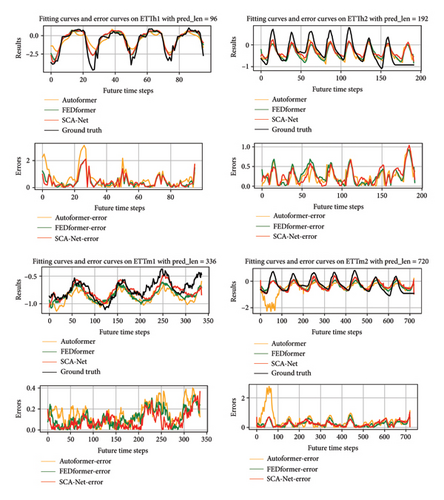
The prediction results on the ETT dataset for horizons of 96, 192, 336, and 720 are illustrated in Figure 6. It can be observed that the proposed model consistently achieves superior alignment with the actual values, especially at peak and valley points. Furthermore, the accompanying error plots indicate that the model maintains the lowest error levels overall, highlighting its improved performance.
4.4. Univariate Results
Extensive experiments on univariate forecasting were also conducted. In comparison to the baseline FEDformer, as depicted in Table 2, the SCA-Net achieved the best predictive results across all datasets and prediction lengths, with the overall MSE and MAE decreasing by 15.6% and 10.2%, respectively. Analyzing different prediction lengths, for a prediction length of 96, the SCA-Net exhibited a 20.5% decrease in overall MSE and a 12.4% decrease in overall MAE; for a prediction length of 192, the overall MSE and MAE decreased by 14.1% and 9.6%, respectively; and for a prediction length of 336, the overall MSE and MAE decreased by 14.4% and 9%, respectively. Based on this analysis, it is evident that the proposed model achieved excellent predictive performance in univariate forecasting. On the ETT dataset, the MSE and MAE decreased by 11.1% and 7.7%, respectively; on the Electricity dataset, the MSE and MAE reduced by 11.4% and 7.7%, respectively; on the Exchange dataset, the MSE and MAE dropped by 28.5% and 25.9%, respectively; on the Traffic dataset, the MSE and MAE declined by 20.8% and 12.8%, respectively; and on the ILI dataset, the MSE and MAE decreased by 13.2% and 7%, respectively. Overall, the SCA-Net exhibited considerable performance improvements in univariate forecasting tasks across different prediction lengths and datasets. Consequently, the presented method could be considered to be applicable in various scenarios. Through extensive experimental validation, the SCA-Net demonstrated particularly good performance improvements compared to other forecasting models with specific datasets or in specific scenarios. This indicates that the SCA-Net possesses good versatility and performance advantages when addressing time-series forecasting problems.
| Datasets | Methods metrics | SCA-Net | FEDformer | Autoformer | Informer | LogTrans | Reformer | ||||||
|---|---|---|---|---|---|---|---|---|---|---|---|---|---|
| MSE | MAE | MSE | MAE | MSE | MAE | MSE | MAE | MSE | MAE | MSE | MAE | ||
| ETTh1 | 96 | 0.070 | 0.205 | 0.079 | 0.215 | 0.071 | 0.206 | 0.193 | 0.377 | 0.283 | 0.468 | 0.532 | 0.569 |
| 192 | 0.084 | 0.224 | 0.104 | 0.245 | 0.114 | 0.262 | 0.217 | 0.395 | 0.234 | 0.409 | 0.568 | 0.575 | |
| 336 | 0.098 | 0.248 | 0.119 | 0.270 | 0.107 | 0.258 | 0.202 | 0.381 | 0.386 | 0.546 | 0.635 | 0.589 | |
| 720 | 0.115 | 0.263 | 0.142 | 0.299 | 0.126 | 0.283 | 0.183 | 0.355 | 0.475 | 0.628 | 0.762 | 0.666 | |
| ETTh2 | 96 | 0.118 | 0.263 | 0.128 | 0.271 | 0.153 | 0.306 | 0.213 | 0.373 | 0.217 | 0.379 | 1.411 | 0.838 |
| 192 | 0.167 | 0.317 | 0.185 | 0.330 | 0.204 | 0.351 | 0.227 | 0.387 | 0.281 | 0.429 | 5.658 | 1.671 | |
| 336 | 0.218 | 0.370 | 0.231 | 0.378 | 0.246 | 0.389 | 0.242 | 0.401 | 0.293 | 0.437 | 4.777 | 1.582 | |
| 720 | 0.259 | 0.408 | 0.278 | 0.420 | 0.268 | 0.409 | 0.291 | 0.439 | 0.218 | 0.387 | 2.042 | 1.039 | |
| ETTm1 | 96 | 0.032 | 0.136 | 0.033 | 0.140 | 0.056 | 0.183 | 0.109 | 0.277 | 0.049 | 0.171 | 0.296 | 0.355 |
| 192 | 0.054 | 0.178 | 0.058 | 0.186 | 0.081 | 0.216 | 0.151 | 0.310 | 0.157 | 0.317 | 0.429 | 0.474 | |
| 336 | 0.073 | 0.212 | 0.084 | 0.231 | 0.076 | 0.218 | 0.427 | 0.591 | 0.289 | 0.459 | 0.585 | 0.583 | |
| 720 | 0.087 | 0.185 | 0.102 | 0.250 | 0.110 | 0.267 | 0.438 | 0.586 | 0.430 | 0.579 | 0.782 | 0.730 | |
| ETTm2 | 96 | 0.060 | 0.183 | 0.067 | 0.198 | 0.065 | 0.189 | 0.088 | 0.225 | 0.075 | 0.208 | 0.076 | 0.214 |
| 192 | 0.096 | 0.236 | 0.102 | 0.245 | 0.118 | 0.256 | 0.132 | 0.283 | 0.129 | 0.275 | 0.132 | 0.290 | |
| 336 | 0.123 | 0.269 | 0.130 | 0.279 | 0.154 | 0.305 | 0.180 | 0.336 | 0.154 | 0.302 | 0.160 | 0.312 | |
| 720 | 0.158 | 0.281 | 0.178 | 0.325 | 0.182 | 0.335 | 0.300 | 0.435 | 0.160 | 0.321 | 0.168 | 0.335 | |
| Electricity | 96 | 0.219 | 0.334 | 0.253 | 0.370 | 0.341 | 0.438 | 0.258 | 0.367 | 0.288 | 0.393 | 0.275 | 0.379 |
| 192 | 0.255 | 0.360 | 0.282 | 0.386 | 0.345 | 0.428 | 0.285 | 0.388 | 0.432 | 0.483 | 0.304 | 0.402 | |
| 336 | 0.309 | 0.402 | 0.346 | 0.431 | 0.406 | 0.470 | 0.336 | 0.423 | 0.430 | 0.483 | 0.370 | 0.448 | |
| 720 | 0.371 | 0.446 | 0.422 | 0.484 | 0.565 | 0.581 | 0.607 | 0.599 | 0.491 | 0.531 | 0.460 | 0.511 | |
| Traffic | 96 | 0.144 | 0.226 | 0.207 | 0.312 | 0.246 | 0.346 | 0.257 | 0.353 | 0.226 | 0.317 | 0.313 | 0.383 |
| 192 | 0.153 | 0.238 | 0.205 | 0.312 | 0.266 | 0.370 | 0.299 | 0.376 | 0.314 | 0.408 | 0.386 | 0.453 | |
| 336 | 0.152 | 0.233 | 0.219 | 0.323 | 0.263 | 0.371 | 0.312 | 0.387 | 0.387 | 0.453 | 0.423 | 0.468 | |
| 720 | 0.177 | 0.259 | 0.244 | 0.344 | 0.269 | 0.372 | 0.366 | 0.436 | 0.437 | 0.491 | 0.378 | 0.433 | |
| Exchange | 96 | 0.098 | 0.239 | 0.154 | 0.304 | 0.241 | 0.387 | 1.327 | 0.944 | 0.237 | 0.377 | 0.298 | 0.444 |
| 192 | 0.218 | 0.356 | 0.286 | 0.420 | 0.300 | 0.369 | 1.258 | 0.924 | 0.738 | 0.619 | 0.777 | 0.719 | |
| 336 | 0.417 | 0.492 | 0.511 | 0.555 | 0.509 | 0.524 | 2.179 | 1.296 | 2.018 | 1.070 | 1.833 | 1.128 | |
| 720 | 1.051 | 0.795 | 1.301 | 0.879 | 1.260 | 0.867 | 1.280 | 0.953 | 2.405 | 1.175 | 1.203 | 0.956 | |
| ILI | 24 | 0.554 | 0.550 | 0.708 | 0.627 | 0.948 | 0.732 | 5.282 | 2.050 | 3.607 | 1.662 | 3.838 | 1.720 |
| 36 | 0.525 | 0.570 | 0.584 | 0.617 | 0.634 | 0.650 | 4.554 | 1.916 | 2.407 | 1.362 | 2.934 | 1.520 | |
| 48 | 0.628 | 0.654 | 0.717 | 0.697 | 0.791 | 0.752 | 4.273 | 1.846 | 3.106 | 1.575 | 3.755 | 1.749 | |
| 60 | 0.780 | 0.752 | 0.855 | 0.774 | 0.874 | 0.797 | 5.214 | 2.057 | 3.698 | 1.733 | 4.162 | 1.847 | |
- Note: A lower MSE/MAE indicates better performance, and bold/italic indicates the best/second.
4.5. Ablation Experiments
In this work, we performed ablation experiments to assess the contribution of the proposed modules to the model’s performance. The key modules under investigation include the SCASeriesDecomp, FPCA, MSDC, and TFB. Experiments were designed from different perspectives to assess the impact of each module.
4.5.1. Ablation Experiment on SCASeriesDecomp
First, to verify the effectiveness of the SCASeriesDecomp, two methods were employed for validation while keeping all other parameters unchanged. The first method replaced the SCASeriesDecomp with Autoformer’s SeriesDecomp, resulting in the SCA-Net-v1. This method aims to verify whether the extraction of seasonality and trends would be affected when the seasonal cycles could not be accurately identified. The second method replaced the SCASeriesDecomp with FEDformer’s MOEDecomp, resulting in the SCA-Net-v2. This was used to verify that the method of merging multiple pooling window weights was not effective when an accurate pooling window could not be found. Detailed findings from the experiment can be found in Table 3.
| Methods | Dataset metrics | ETTh1 | ETTh2 | ETTm1 | ETTm2 | ||||||||||||
|---|---|---|---|---|---|---|---|---|---|---|---|---|---|---|---|---|---|
| 96 | 192 | 336 | 720 | 96 | 192 | 336 | 720 | 96 | 192 | 336 | 720 | 96 | 192 | 336 | 720 | ||
| SCA-Net | MSE | 0.361 | 0.402 | 0.435 | 0.460 | 0.331 | 0.410 | 0.445 | 0.453 | 0.313 | 0.368 | 0.401 | 0.455 | 0.183 | 0.254 | 0.316 | 0.418 |
| MAE | 0.406 | 0.433 | 0.452 | 0.476 | 0.375 | 0.426 | 0.457 | 0.471 | 0.365 | 0.412 | 0.435 | 0.460 | 0.275 | 0.317 | 0.357 | 0.413 | |
| SCA-Net-v1 | MSE | 0.363 | 0.404 | 0.442 | 0.476 | 0.333 | 0.419 | 0.448 | 0.461 | 0.344 | 0.379 | 0.413 | 0.467 | 0.199 | 0.261 | 0.327 | 0.419 |
| MAE | 0.408 | 0.435 | 0.455 | 0.484 | 0.378 | 0.428 | 0.459 | 0.475 | 0.393 | 0.413 | 0.438 | 0.474 | 0.286 | 0.319 | 0.362 | 0.415 | |
| SCA-Net-v2 | MSE | 0.368 | 0.403 | 0.438 | 0.461 | 0.335 | 0.412 | 0.449 | 0.486 | 0.339 | 0.387 | 0.419 | 0.456 | 0.202 | 0.265 | 0.326 | 0.444 |
| MAE | 0.408 | 0.434 | 0.456 | 0.479 | 0.379 | 0.428 | 0.462 | 0.491 | 0.394 | 0.427 | 0.446 | 0.467 | 0.285 | 0.323 | 0.363 | 0.434 | |
- Note: SCA-Net-v1 employs the SeriesDecomp proposed by Autoformer to replace the SCASeriesDecomp, while SCA-net-v2 uses the MOESeriesDecomp proposed by FEDformer to replace the SCASeriesDecomp (lower MSE/MAE indicates better performance, with bold and italic representing the best and second-best results).
According to the experimental findings illustrated in Table 3, the proposed SCASeriesDecomp outperforms the trend-seasonality decomposition approaches employed by Autoformer and FEDformer. Traditional decomposition methods often face difficulties in accurately distinguishing trend and seasonal components when the seasonal cycle is not clearly defined. In contrast, leveraging the results from Fourier spectrum analysis, our approach effectively identifies the exact seasonal cycle embedded in the time-series data. This enables a more accurate separation of the trend component and reliable extraction of seasonal features.
To further validate the effectiveness of using only the Top1 frequency for period estimation in SCA-Net, we designed a set of comparative experiments to assess the impact of different frequency selection strategies on period estimation performance. Detailed experiments were conducted on four publicly available time series datasets (ETTh1, ETTh2, ETTm1, anf ETTm2) and four different prediction horizons (96, 192, 336, and 720), with the evaluation metrics being MSE and MAE. The original SCA-Net method uses only the Top1 frequency in the spectrum to calculate the period, treating it as an average pooling window. As shown in Table 4, to further verify whether this selection is reasonable, we conducted comparative experiments based on the original model structure and parameters, with the following strategies: Top2, where the second most significant frequency in the spectrum is chosen for the period; Top3, where the third most significant frequency is selected; and mean, where the mean importance of the Top1, Top2, and Top3 frequencies is computed and used as the period.
| Methods | Dataset metrics | ETTh1 | ETTh2 | ETTm1 | ETTm2 | ||||||||||||
|---|---|---|---|---|---|---|---|---|---|---|---|---|---|---|---|---|---|
| 96 | 192 | 336 | 720 | 96 | 192 | 336 | 720 | 96 | 192 | 336 | 720 | 96 | 192 | 336 | 720 | ||
| SCA-Net | MSE | 0.361 | 0.402 | 0.435 | 0.460 | 0.331 | 0.410 | 0.445 | 0.453 | 0.331 | 0.368 | 0.401 | 0.455 | 0.183 | 0.254 | 0.316 | 0.418 |
| MAE | 0.406 | 0.433 | 0.452 | 0.476 | 0.375 | 0.426 | 0.457 | 0.471 | 0.365 | 0.412 | 0.435 | 0.460 | 0.275 | 0.317 | 0.357 | 0.413 | |
| Top2 | MSE | 0.371 | 0.409 | 0.447 | 0.510 | 0.337 | 0.425 | 0.446 | 0.450 | 0.335 | 0.370 | 0.387 | 0.442 | 0.191 | 0.256 | 0.327 | 0.421 |
| MAE | 0.412 | 0.438 | 0.459 | 0.518 | 0.380 | 0.433 | 0.458 | 0.470 | 0.382 | 0.415 | 0.426 | 0.459 | 0.282 | 0.321 | 0.366 | 0.422 | |
| Top3 | MSE | 0.394 | 0.432 | 0.466 | 0.507 | 0.332 | 0.422 | 0.457 | 0.441 | 0.336 | 0.381 | 0.393 | 0.452 | 0.201 | 0.262 | 0.324 | 0.419 |
| MAE | 0.434 | 0.455 | 0.472 | 0.511 | 0.375 | 0.432 | 0.466 | 0.477 | 0.388 | 0.417 | 0.429 | 0.461 | 0.285 | 0.320 | 0.362 | 0.420 | |
| Mean | MSE | 0.381 | 0.427 | 0.456 | 0.496 | 0.331 | 0.411 | 0.464 | 0.444 | 0.333 | 0.369 | 0.394 | 0.450 | 0.185 | 0.256 | 0.320 | 0.419 |
| MAE | 0.422 | 0.446 | 0.462 | 0.502 | 0.376 | 0.427 | 0.476 | 0.468 | 0.381 | 0.413 | 0.429 | 0.462 | 0.278 | 0.319 | 0.360 | 0.418 | |
- Note: The SCA-Net method uses only the Top1 frequency in the spectrum to calculate the period. The Top2 strategy selects the second most significant frequency in the spectrum as the period. The Top3 strategy selects the third most significant frequency as the period. The mean strategy calculates the average importance of the Top1, Top2, and Top3 frequencies to determine the period (lower MSE/MAE indicates better performance, with bold and italic representing the best and second-best results).
The experimental results shown in Table 4 indicate that in most cases, the SCA-Net model using the Top1 frequency achieved the best or nearly the best results, especially for shorter prediction horizons (96, 192), where the performance of the Top1 strategy was significantly better than the other strategies. For some datasets and longer prediction horizons (336 and 720), the results of the Top2 and mean strategies were close to or even slightly better than Top1, suggesting that in certain scenarios, considering the mean of the Top2 or Top3 frequencies can sometimes improve model performance, especially when the importance of different frequencies is relatively similar. However, using the Top3 frequency generally led to worse results, indicating that the order of frequency importance plays a significant role in model performance for period estimation. The introduction of lower-ranked frequencies can lead to larger errors. Although the mean strategy exhibited stable performance on certain datasets and prediction horizons, it did not show a clear advantage overall, with the Top1 frequency still being the most effective and efficient choice. Through this set of comparative experiments, we validated the rationality of using only the Top1 frequency for period estimation. While in some cases, considering the mean of the Top2 or Top3 frequencies may provide similar performance, overall, Top1 remains the most robust and optimal choice.
4.5.2. Ablation Experiment on FPCA
In validating the effectiveness of the FPCA, the effectiveness of odd–even decomposition compared to randomly selecting Fourier components was first examined. The FEB in FEDformer was replaced with FPCA-v1, removing the feature correction component of the FPCA, resulting in the FEDformer-v1. If the predictive performance improved, it would indicate that the odd–even decomposition method was superior to the feature correction method. As displayed in Table 5, the detailed results of the experiment are provided. Next, the necessity of adding odd–even fusion terms for feature correction was assessed. Here, the odd–even component was removed from the FPCA in the SCA-Net, to obtain SCA-Net-v3. Without changing other parameters, the predictive performance of SCA-Net-v3 considerably decreased compared to the SCA-Net, suggesting that adding an odd–even fusion term for feature correction on top of odd–even decomposition was effective. The detailed results of the experiment are provided in Table 6.
| Methods | Dataset metrics | ETTh1 | ETTh2 | ETTm1 | ETTm2 | ||||||||||||
|---|---|---|---|---|---|---|---|---|---|---|---|---|---|---|---|---|---|
| 96 | 192 | 336 | 720 | 96 | 192 | 336 | 720 | 96 | 192 | 336 | 720 | 96 | 192 | 336 | 720 | ||
| FEDformer | MSE | 0.376 | 0.420 | 0.459 | 0.506 | 0.346 | 0.429 | 0.496 | 0.463 | 0.379 | 0.426 | 0.445 | 0.543 | 0.203 | 0.269 | 0.325 | 0.421 |
| MAE | 0.419 | 0.448 | 0.465 | 0.507 | 0.388 | 0.439 | 0.487 | 0.474 | 0.419 | 0.441 | 0.459 | 0.490 | 0.287 | 0.328 | 0.366 | 0.415 | |
| FEDformer-v1 | MSE | 0.372 | 0.418 | 0.455 | 0.502 | 0.336 | 0.427 | 0.490 | 0.421 | 0.365 | 0.407 | 0.442 | 0.512 | 0.189 | 0.253 | 0.323 | 0.420 |
| MAE | 0.413 | 0.441 | 0.464 | 0.504 | 0.382 | 0.433 | 0.485 | 0.472 | 0.408 | 0.435 | 0.456 | 0.483 | 0.280 | 0.322 | 0.364 | 0.413 | |
- Note: FEDformer-v1 uses FPCA-v1 to replace the FEB, where FPCA-v1 represents the FPCA with the feature correction part removed (lower MSE/MAE indicates better performance, with bold and italic representing the best and second-best results).
| Methods | Dataset metrics | ETTh1 | ETTh2 | ETTm1 | ETTm2 | ||||||||||||
|---|---|---|---|---|---|---|---|---|---|---|---|---|---|---|---|---|---|
| 96 | 192 | 336 | 720 | 96 | 192 | 336 | 720 | 96 | 192 | 336 | 720 | 96 | 192 | 336 | 720 | ||
| SCA-Net | MSE | 0.361 | 0.402 | 0.435 | 0.460 | 0.331 | 0.410 | 0.445 | 0.453 | 0.313 | 0.368 | 0.401 | 0.455 | 0.183 | 0.254 | 0.316 | 0.418 |
| MAE | 0.406 | 0.433 | 0.452 | 0.476 | 0.375 | 0.426 | 0.457 | 0.471 | 0.365 | 0.412 | 0.435 | 0.460 | 0.275 | 0.317 | 0.357 | 0.413 | |
| SCA-Net-v3 | MSE | 0.364 | 0.407 | 0.443 | 0.476 | 0.332 | 0.413 | 0.446 | 0.460 | 0.316 | 0.372 | 0.402 | 0.456 | 0.184 | 0.256 | 0.324 | 0.432 |
| MAE | 0.409 | 0.438 | 0.457 | 0.481 | 0.377 | 0.429 | 0.458 | 0.475 | 0.375 | 0.413 | 0.437 | 0.461 | 0.276 | 0.318 | 0.366 | 0.424 | |
- Note: SCA-Net uses FPCA-v1 to replace the FPCA, where FPCA-v1 represents the FPCA with the feature correction part removed (lower MSE/MAE indicates better performance, with bold and italic representing the best and second-best results).
According to the results presented in Table 5, FEDformer-v1 achieves better predictive accuracy than the original FEDformer. This suggests that splitting the time series into odd and even components and performing frequency-domain feature extraction is more efficient than randomly choosing a set number of Fourier components, thus supporting the effectiveness of the proposed odd–even decomposition approach. In addition, as shown in Table 6, the elimination of the FPCA’s feature correction module leads to a decline in the overall forecasting performance. This finding highlights the importance of incorporating the designed odd–even fusion terms for effective feature adjustment.
To validate the effectiveness of the FPCA method we proposed, we designed a series of experiments using different processing methods for comparative analysis. Specifically, we conducted practical experiments with the odd, even, and odd–even fusion terms (similar to the moving average method) to evaluate their performance in time-series prediction tasks. In the experiments, we used the ETTh1 and ETTh2 datasets and trained and tested four methods: using only the odd-numbered data (Odd_Term), using only the even-numbered data (Even_Term), combining the odd and even terms (Mean_Term, which is similar to the moving average method), and the traditional moving average method. The main purpose of these methods was to verify whether the fusion of odd and even terms could effectively capture the periodic and trend features in the time-series data.
The experimental results showed in Table 7 that the odd term (Odd_Term) performed poorly across all time horizons, especially for longer time steps (e.g., 720 steps), where the prediction error was large. This suggests that using only the odd-numbered data may not fully capture the information in the time series data. The even term (Even_Term) performed better for shorter time steps (e.g., 96 steps), but the error increased as the time steps grew, indicating that while the even term can capture long-term trends in the data, it is less effective at handling local fluctuations and periodic variations in the data. In contrast, the odd–even fusion term (Mean_Term) performed well across all time horizons, with its prediction errors significantly lower than those of other methods, particularly for longer time steps. This indicates that the fusion of odd and even terms provides a more comprehensive representation of the periodic, trend, and fluctuation features in the time-series data, thereby improving prediction accuracy. The traditional moving average method performed relatively poorly across all time steps, especially for the longer time step (720 steps), where the prediction error was large. This suggests that while the moving average method effectively smooths the data and reduces noise, it oversimplifies the dynamic changes in the data and fails to capture important periodic features and local fluctuations, which reduces prediction accuracy. In conclusion, the experimental results confirm the effectiveness of the FPCA method, particularly the advantage of the odd–even fusion term in time-series prediction. Compared to methods that use only the odd or even terms, the odd–even fusion term not only better captures the trends and periodic variations in the data but also improves prediction accuracy, especially for longer time steps. In contrast, the traditional moving average method, due to its oversimplification of data dynamics, is unable to effectively handle the complex variations in the time-series data, leading to poor performance in time-series prediction tasks. Therefore, the FPCA method based on the odd–even fusion term offers a more accurate and effective solution for time-series prediction tasks.
| Methods | Dataset metrics | ETTh1 | ETTh2 | ||||||
|---|---|---|---|---|---|---|---|---|---|
| 96 | 192 | 336 | 720 | 96 | 192 | 336 | 720 | ||
| SCA-Net | MSE | 0.361 | 0.402 | 0.435 | 0.460 | 0.331 | 0.410 | 0.445 | 0.453 |
| MAE | 0.406 | 0.433 | 0.452 | 0.476 | 0.375 | 0.426 | 0.457 | 0.471 | |
| Odd_Term | MSE | 0.384 | 0.436 | 0.464 | 0.480 | 0.331 | 0.411 | 0.445 | 0.467 |
| MAE | 0.423 | 0.452 | 0.466 | 0.491 | 0.377 | 0.426 | 0.459 | 0.478 | |
| Even_Term | MSE | 0.379 | 0.420 | 0.451 | 0.477 | 0.332 | 0.412 | 0.464 | 0.468 |
| MAE | 0.417 | 0.444 | 0.457 | 0.487 | 0.378 | 0.426 | 0.475 | 0.479 | |
| Mean_Term | MSE | 0.378 | 0.419 | 0.450 | 0.476 | 0.333 | 0.411 | 0.464 | 0.464 |
| MAE | 0.416 | 0.443 | 0.456 | 0.487 | 0.379 | 0.426 | 0.475 | 0.473 | |
- Note: Odd_Term and Even_Term represent models that perform frequency-domain extraction using only the odd- or even-indexed time steps, respectively. Mean_Term denotes the simple average of odd and even features, similar to a moving average method (lower MSE/MAE indicates better performance, with bold and italic representing the best and second-best results).
4.5.3. Ablation Experiment on MSDC
Next, we evaluate the impact of MSDC to verify the importance of capturing local dependencies within seasonal cycles. To achieve this, we adopt two complementary strategies. Approach 1: We embed the MSDC module into both components of FEDformer, resulting in FEDformer-v2. If this modified model demonstrates enhanced forecasting performance, it validates the value of explicitly modeling seasonal cycles. Approach 2: We ablate the MSDC component from the architecture, retaining only the FPCA module for extracting global characteristics. A noticeable decline in performance in this case would further support the necessity of integrating both global and local modeling mechanisms tailored to seasonal structures.
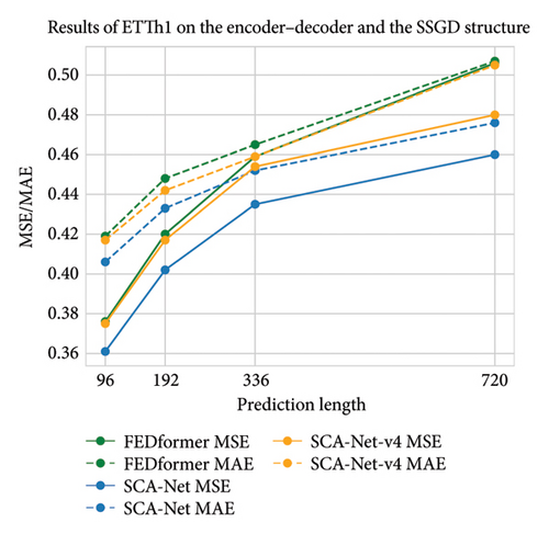
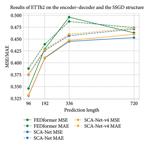
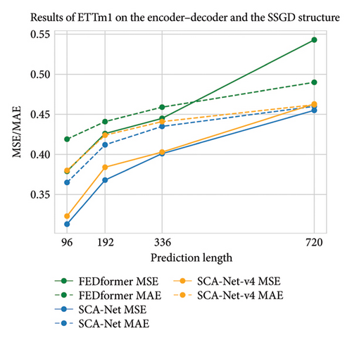
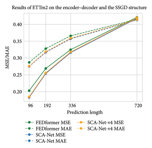
The experimental outcomes presented in Tables 8 and 9 suggest that MSDC contributes substantially to enhancing predictive accuracy. This confirms the rationality of incorporating seasonal pattern modeling and capturing local temporal dependencies. Moreover, evidence from Table 9 and Figure 7 shows that even in the absence of MSDC, our framework, featuring a lightweight single-layer, one-step generative decoder, outperforms the encoder–decoder–based FEDformer. These results affirm the efficacy of the proposed SSGD design and underscore its strong potential for future development.
| Methods | Dataset metrics | ETTh1 | ETTh2 | ETTm1 | ETTm2 | ||||||||||||
|---|---|---|---|---|---|---|---|---|---|---|---|---|---|---|---|---|---|
| 96 | 192 | 336 | 720 | 96 | 192 | 336 | 720 | 96 | 192 | 336 | 720 | 96 | 192 | 336 | 720 | ||
| FEDformer | MSE | 0.376 | 0.420 | 0.459 | 0.506 | 0.346 | 0.429 | 0.496 | 0.463 | 0.379 | 0.426 | 0.445 | 0.543 | 0.203 | 0.269 | 0.325 | 0.421 |
| MAE | 0.419 | 0.448 | 0.465 | 0.507 | 0.388 | 0.439 | 0.487 | 0.474 | 0.419 | 0.441 | 0.459 | 0.490 | 0.287 | 0.328 | 0.366 | 0.415 | |
| FEDformer-v2 | MSE | 0.373 | 0.415 | 0.453 | 0.487 | 0.338 | 0.426 | 0.486 | 0.456 | 0.355 | 0.394 | 0.420 | 0.471 | 0.197 | 0.265 | 0.323 | 0.419 |
| MAE | 0.412 | 0.441 | 0.461 | 0.497 | 0.380 | 0.433 | 0.483 | 0.473 | 0.402 | 0.427 | 0.441 | 0.465 | 0.285 | 0.326 | 0.362 | 0.413 | |
- Note: FEDformer-v2 integrates the MSDC directly into FEDformer (lower MSE/MAE indicates better performance, with bold and italic representing the best and second-best results).
| Methods | Dataset metrics | ETTh1 | ETTh2 | ETTm1 | ETTm2 | ||||||||||||
|---|---|---|---|---|---|---|---|---|---|---|---|---|---|---|---|---|---|
| 96 | 192 | 336 | 720 | 96 | 192 | 336 | 720 | 96 | 192 | 336 | 720 | 96 | 192 | 336 | 720 | ||
| FEDformer | MSE | 0.376 | 0.420 | 0.459 | 0.506 | 0.346 | 0.429 | 0.496 | 0.463 | 0.379 | 0.426 | 0.445 | 0.543 | 0.203 | 0.269 | 0.325 | 0.421 |
| MAE | 0.419 | 0.448 | 0.465 | 0.507 | 0.388 | 0.439 | 0.487 | 0.474 | 0.419 | 0.441 | 0.459 | 0.490 | 0.287 | 0.328 | 0.366 | 0.415 | |
| SCA-Net | MSE | 0.361 | 0.402 | 0.435 | 0.460 | 0.331 | 0.410 | 0.445 | 0.453 | 0.313 | 0.368 | 0.401 | 0.455 | 0.183 | 0.254 | 0.316 | 0.418 |
| MAE | 0.406 | 0.433 | 0.452 | 0.476 | 0.375 | 0.426 | 0.457 | 0.471 | 0.365 | 0.412 | 0.435 | 0.460 | 0.275 | 0.317 | 0.357 | 0.413 | |
| SCA-Net-v4 | MSE | 0.375 | 0.417 | 0.454 | 0.480 | 0.332 | 0.411 | 0.447 | 0.478 | 0.323 | 0.384 | 0.403 | 0.463 | 0.185 | 0.256 | 0.318 | 0.432 |
| MAE | 0.417 | 0.442 | 0.459 | 0.505 | 0.376 | 0.428 | 0.460 | 0.485 | 0.380 | 0.424 | 0.441 | 0.462 | 0.276 | 0.319 | 0.359 | 0.426 | |
- Note: SCA-Net-v4 directly removes the MSDC from SCA-Net (lower MSE/MAE indicates better performance, with bold and italic representing the best and second-best results).
4.5.4. Ablation Experiment on TFB
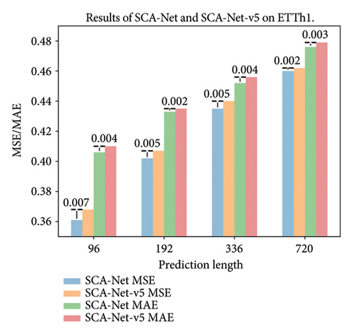
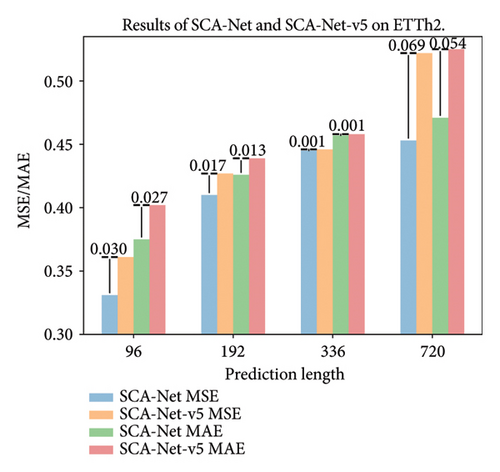
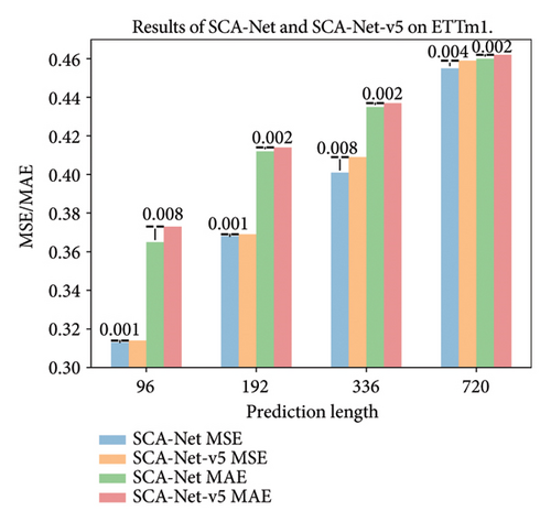
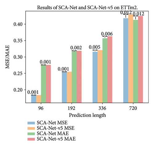
Next, we validated the effectiveness of the TFB, specifically focusing on the regression of the trend components. In SCA-Net-v5, we refrained from applying regression to the trend components decomposed by the SCASeriesDecomp. Instead, we performed a simple addition of the decomposed trend components with the final seasonal components through residual connections. If the predictive performance of SCA-Net-v5 deteriorated considerably compared to the SCA-Net, it would indicate that modeling the trend components through regression was effective. Table 10 highlights the specific outcomes of the experiment.
| Methods | Dataset metrics | ETTh1 | ETTh2 | ETTm1 | ETTm2 | ||||||||||||
|---|---|---|---|---|---|---|---|---|---|---|---|---|---|---|---|---|---|
| 96 | 192 | 336 | 720 | 96 | 192 | 336 | 720 | 96 | 192 | 336 | 720 | 96 | 192 | 336 | 720 | ||
| SCA-Net | MSE | 0.361 | 0.402 | 0.435 | 0.460 | 0.331 | 0.410 | 0.445 | 0.453 | 0.313 | 0.368 | 0.401 | 0.455 | 0.183 | 0.254 | 0.316 | 0.418 |
| MAE | 0.406 | 0.433 | 0.452 | 0.476 | 0.375 | 0.426 | 0.457 | 0.471 | 0.365 | 0.412 | 0.435 | 0.460 | 0.275 | 0.317 | 0.357 | 0.413 | |
| SCA-Net-v5 | MSE | 0.368 | 0.407 | 0.440 | 0.462 | 0.361 | 0.427 | 0.446 | 0.522 | 0.314 | 0.369 | 0.409 | 0.459 | 0.183 | 0.255 | 0.321 | 0.430 |
| MAE | 0.410 | 0.435 | 0.456 | 0.479 | 0.402 | 0.439 | 0.458 | 0.525 | 0.373 | 0.414 | 0.437 | 0.462 | 0.276 | 0.319 | 0.363 | 0.425 | |
- Note: SCA-Net-v5 directly removes TFB from SCA-Net (lower MSE/MAE indicates better performance, with bold and italic representing the best and second-best results).
It can be seen from Table 10 that the original SCA-Net, which incorporates trend regression, achieves better forecasting performance than SCA-Net-v5. In addition, by plotting the difference bar chart, as shown in Figure 8, it provides a clearer visualization of the predictive differences between the SCA-Net-v5 and SCA-Net. This allows one to gain a more precise understanding of the effectiveness of regression processing for trend components. In time series, trend components typically encompass long-term and global patterns, with fully connected layers excelling in establishing global correlations across the entire feature set. Consequently, opting for regression methods can help in capturing global correlations among features within trend components, thereby enhancing the effectiveness of their modeling. Moreover, regression methods offer advantages in handling continuous data and predicting future trends, facilitating better fitting and forecasting of long-term trend changes. The integration of trend components processed through regression with seasonal components through residual connections can help compensate for missing trend information during the seasonal-trend decomposition process in time-series data. This integration enables the model to better capture the correlations between trend and seasonal components, thereby improving the overall feature set. This integration allows the model to more effectively capture the relationships between trend and seasonal components, leading to an improved feature set. By strengthening the connection between these components, residual connections can help fill information gaps, ultimately improving the model’s accuracy and robustness when handling complex time-series data.
4.6. Performance Analysis as Strong Plugins
Strong plugins refer to additional components or modules that can be integrated into existing models, aimed at significantly enhancing model performance, particularly by addressing specific limitations or weaknesses of the base model. In this study, we focus on analyzing the impact of SCASeriesDecomp and FPCA as strong plugins on the performance of the PatchTST model. The experimental results, shown in Table 11, demonstrate that integrating these two plugins into the model leads to significant performance improvements. Specifically, the introduction of SCASeriesDecomp and FPCA results in a general reduction in predictive errors, validating their effectiveness in enhancing model accuracy. In the ETTh1 dataset, the inclusion of SCASeriesDecomp and FPCA reduces the overall MSE from 0.449 to 0.437 and 0.435, respectively, and the overall MAE from 0.449 to 0.439 and 0.437. This trend is similarly observed across other datasets, further confirming their efficacy. In summary, SCASeriesDecomp and FPCA serve as valuable plugins that notably enhance the performance of PatchTST on diverse datasets and forecasting periods. This discovery offers a robust foundation for future work aimed at incorporating these plugins into other models to improve predictive performance.
| Methods | Model metrics | PatchTST | +SCASeriesDecomp | +FPCA | |||
|---|---|---|---|---|---|---|---|
| MSE | MAE | MSE | MAE | MSE | MAE | ||
| ETTh1 | 96 | 0.379 | 0.399 | 0.378 | 0.398 | 0.375 | 0.395 |
| 192 | 0.424 | 0.431 | 0.430 | 0.432 | 0.429 | 0.429 | |
| 336 | 0.469 | 0.458 | 0.468 | 0.452 | 0.459 | 0.445 | |
| 720 | 0.524 | 0.506 | 0.473 | 0.472 | 0.478 | 0.479 | |
| AVG | 0.449 | 0.449 | 0.437 | 0.439 | 0.435 | 0.437 | |
| ETTh2 | 96 | 0.300 | 0.353 | 0.293 | 0.343 | 0.299 | 0.351 |
| 192 | 0.385 | 0.409 | 0.377 | 0.395 | 0.371 | 0.394 | |
| 336 | 0.423 | 0.438 | 0.413 | 0.426 | 0.422 | 0.433 | |
| 720 | 0.432 | 0.453 | 0.429 | 0.448 | 0.425 | 0.444 | |
| AVG | 0.385 | 0.413 | 0.378 | 0.403 | 0.379 | 0.406 | |
| ETTm1 | 96 | 0.326 | 0.366 | 0.325 | 0.363 | 0.320 | 0.363 |
| 192 | 0.375 | 0.393 | 0.370 | 0.390 | 0.367 | 0.388 | |
| 336 | 0.399 | 0.408 | 0.397 | 0.406 | 0.397 | 0.405 | |
| 720 | 0.457 | 0.444 | 0.456 | 0.443 | 0.456 | 0.443 | |
| AVG | 0.389 | 0.403 | 0.387 | 0.401 | 0.385 | 0.400 | |
| ETTm2 | 96 | 0.183 | 0.267 | 0.176 | 0.259 | 0.178 | 0.261 |
| 192 | 0.245 | 0.304 | 0.243 | 0.303 | 0.244 | 0.303 | |
| 336 | 0.313 | 0.350 | 0.303 | 0.342 | 0.309 | 0.348 | |
| 720 | 0.402 | 0.400 | 0.400 | 0.398 | 0.401 | 0.398 | |
| AVG | 0.286 | 0.330 | 0.281 | 0.326 | 0.283 | 0.328 | |
| Exchange | 96 | 0.096 | 0.215 | 0.084 | 0.201 | 0.088 | 0.207 |
| 192 | 0.181 | 0.303 | 0.176 | 0.297 | 0.180 | 0.301 | |
| 336 | 0.343 | 0.426 | 0.342 | 0.420 | 0.338 | 0.421 | |
| 720 | 0.944 | 0.729 | 0.859 | 0.697 | 0.877 | 0.706 | |
| AVG | 0.391 | 0.418 | 0.365 | 0.404 | 0.371 | 0.409 | |
- Note: Bold indicates the performance improvement when SCASeriesDecomp is inserted into the PatchTST compared to the original PatchTST. Italic indicates the performance improvement when FPCA is inserted into the PatchTST compared to the original PatchTST. AVG indicates the mean performance across four different forecasting horizons for each dataset.
4.7. Parameter Sensitivity Analysis
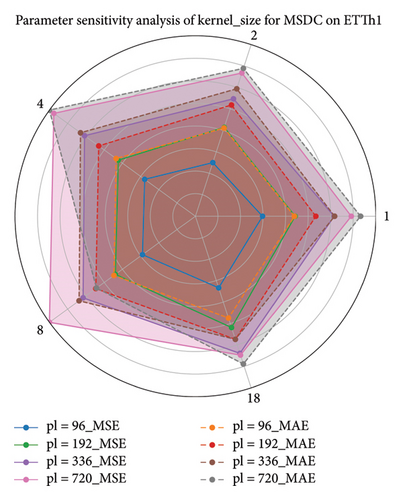
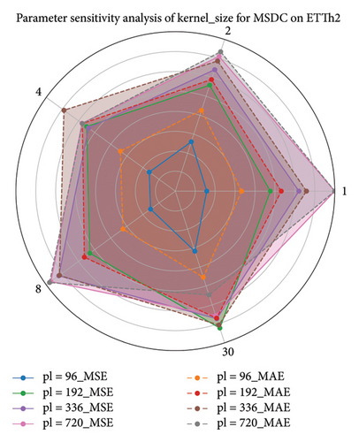
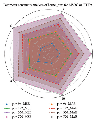
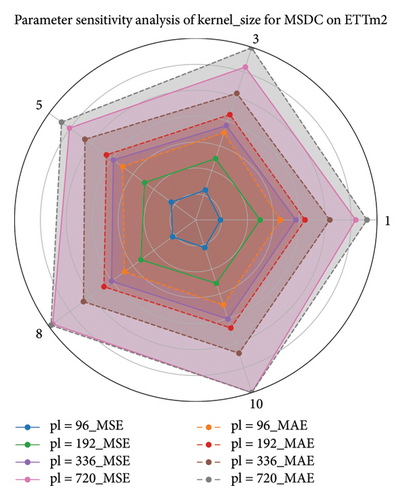
Here, we conducted a sensitivity analysis of the kernel size in the MSDC feature output layer, based on experiments with the ETT datasets. Owing to variations in the seasonal patterns of time series across different datasets, a key objective of the sensitivity analysis on the MSDC’s kernel is to identify the optimal seasonal cycles corresponding to each dataset. This design facilitates precise modeling of temporal periodicity. By modulating the convolutional kernel’s scale, the model can more effectively extract local temporal patterns, increase responsiveness to cyclical fluctuations, and ultimately improve predictive accuracy.
Different kernel scales in the convolutional layer can capture features across varying ranges. Thus, we performed a sensitivity analysis on these parameters using a radar chart, as depicted in Figure 9. As depicted in the radar chart, the choice of kernel scale substantially influences the model’s overall performance. The chart depicts a polygon for each scale, with each vertex representing a specific kernel size. The shape of the polygon reflects the model’s performance at different scales, whereas the convexity and size of the polygon correspond to the model’s performance under different parameter settings. Through this visualization, one can easily evaluate performance fluctuations under changing conditions, which assists in choosing the best kernel size. According to the experimental results, adjusting seasonal cycles according to dataset-specific characteristics is essential. This enables the extraction of accurate local features, which in turn improves feature fusion.
4.8. Complexity Analysis
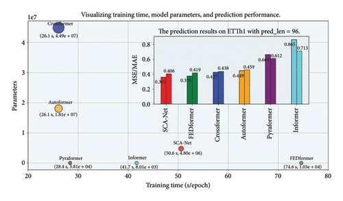
Here, we analyzed the spatiotemporal complexity in detail and conducted experiments on a 3060Ti graphics card. By comparing the training duration and forecasting accuracy of the models at a horizon length of 96 on the ETTh1 dataset, their overall performance can be assessed. A comprehensive evaluation strategy was adopted, taking into account parameter quantity, training duration, and prediction accuracy of the baseline methods to holistically measure model effectiveness. According to the statistics in Table 12, a corresponding visualization was generated in Figure 10, illustrating comparative efficiency and capability. As shown, our model achieves a well-balanced compromise between resource consumption and predictive performance when compared to its counterparts. The importance of focusing on the efficiency of the models in training and inference should be noted, while also considering the model’s expressive power to ensure an adequate representation ability while maintaining reasonable computational costs. However, objectively speaking, the proposed model still exhibits a relatively high overall parameter count compared to other models, which is one of the key problems that needs to be addressed in future work. In future studies, the next step should focus on reducing spatiotemporal complexity while improving forecasting accuracy, thereby further enhancing the practicality and overall effectiveness of the proposed model.
| Methods | SCA-Net | FEDformer | Crossformer | Autoformer | Pyraformer | Informer |
|---|---|---|---|---|---|---|
| Parameters | 4.80e + 06 | 1.03e + 04 | 4.49e + 07 | 1.81e + 07 | 3.81e + 04 | 8.01e + 03 |
| Training time (s/epoch) | 50.6 | 74.6 | 26.1 | 26.1 | 28.4 | 41.7 |
| MSE | 0.361 | 0.376 | 0.427 | 0.449 | 0.664 | 0.865 |
| MAE | 0.406 | 0.419 | 0.438 | 0.459 | 0.612 | 0.713 |
- Note: Highlight in bold represents the lower values for parameters, training time, MSE, and MAE.
5. Conclusions
This paper introduces a SCA-Net. The study aims to address the issue that existing attention mechanisms primarily focus on global modeling while overlooking local correlations between seasonal cycles in time series. By proposing a dual-branch extraction architecture that decomposes time series into trend and seasonal components, we aim to improve prediction accuracy and enhance model interpretability. To improve the model’s ability to learn complex seasonal components, we propose a novel frequency-domain attention module that utilizes even–odd sequence decomposition and refines features in the spectral domain. By incorporating a multiscale dilated convolution structure, the model can effectively capture both long-term temporal patterns and short-term seasonal variations at different resolutions. For relatively straightforward trend components, a regression approach is employed, and their outputs are merged with the seasonal components via residual connections. To tackle the challenge of accurately identifying seasonal cycles in traditional decomposition methods, we propose a seasonally adaptive seasonal-trend decomposition technique that precisely separates time-series signals and extracts key information. The architecture of SCA-Net employs a single-layer generative decoder, deviating from the conventional encoder–decoder structure of transformers. This simplifies the model while enhancing predictive performance. Comprehensive experiments on eight benchmark datasets validate the superior forecasting performance of our model, emphasizing the distinct advantages of SCA-Net in time-series forecasting tasks.
Nomenclature
-
- ANA
-
- Antinuclear antibodies
-
- APC
-
- Antigen-presenting cells
-
- IRF
-
- Interferon regulatory factor
Conflicts of Interest
The authors declare no conflicts of interest.
Funding
This work was supported in part the Joint Fund of the National Natural Science Foundation of China under grant nos. U24A20219, U24A20328, and U22A2033; the National Natural Science Foundation of China under grant no. 62272281; the Special Funds for the Taishan Scholars Project under grant no. tsqn202306274; and the Youth Innovation Technology Project of Higher School in Shandong Province under grant no. 2023KJ212.
Open Research
Data Availability Statement
The data supporting the findings of this study are publicly available at the following sources: ETT dataset: https://github.com/zhouhaoyi/ETDataset; Electricity dataset: https://archive.ics.uci.edu/dataset/321/electricityloaddiagrams20112014; Exchange dataset: https://github.com/laignokun/multivariate-time-series-data; Traffic dataset: https://zenodo.org/record/4656132/; ILI dataset: https://gis.cdc.gov/grasp/fluview/fluportaldashboard.html.


