This paper deals with dynamical analysis of an ecological model. This model includes two logistically growing prey species, namely, Prey X and Prey Y, and the third species Z behaves as the predator, predating both Prey X and Prey Y according to the extended Holling type-II functional response. Furthermore, the effect of fear is incorporated in the growth rate of both species Prey X and Prey Y due to the predator Z. All the biologically possible steady state points are explored, and their local stability as well as global stability is analyzed based on the sample parameters. Next, we investigate the occurrence of local bifurcations around each steady state points by taking the value of the birth rate, death rate, and fear parameter as a bifurcation parameter. Finally, we perform extensive numerical simulations to support the evidence of our analytical results.

1. Introduction

1.1. Motivation and Literature Survey

To understand the dynamics of interaction between prey species and predator species, thousands of prey–predator models have been considered by mathematician authors [1–5]. The important element to represent the dynamics relationship between predator population and prey population is the functional response for the predator, which is defined as the number of consumed prey per predator per unit time [6]. The most useful functional response is the Holling type-II functional response, which is characterized by the decelerating intake rate [7]. Many authors used this type of functional response for modeling the dynamics of interactions between predator and prey [8]. In nature, lions are a real-world example of predator species that consume more than one species of prey, usually a number of large land-based animals, such as antelopes, buffaloes, crocodiles, giraffes, pigs, zebra, wild dogs, and wildebeest. There are some works modeling one predator and multiple preys [6, 7].

Eletterby in [2] discussed the global stability and persistence of a two preys and one predator model. Population dynamics may be affected by many factor such as fear, harvesting, toxicity, stage structure, delay, harvesting, cannibalism, antipredator skills, refuge, infectious illness, and other population-affecting elements of the natural environment [9–12].

Physiological changes of prey population may be caused by predation fears, and these physiological changes may reduce the reproduction of prey population. Zanette et al. [13] showed that the bird reduce 40 percent less offspring by the fear from predator. Wang et al. [14] considered a predator–prey model incorporating fear effect on reproduction of prey individuals; in their study, they noticed that the fear has no impact on the stability of the model when the system incorporate bilinear functional response, but the system becomes stable under fear effect, if it incorporate the Holling type-II functional response, based on their system. Pal et al. [15] considered a prey predator with fear effect and harvesting cooperation; they discussed the stability, Hopf bifurcation, and Bogdanov–Takens bifurcation of the system. Zhang et al. [16] considered an ecological model with fear effect and prey refuge, and they showed that the effect of both factors can stabilize the system. For more results about fear effect, see [9, 17–21]. It is important to study the effect of fear on the dynamics relationship between one predator species and more than one prey species. The aim of the current work is to model the impact of effect of fear on the dynamics of interaction between one predator species and two prey species.

1.2. The Model Formulation

The authors in [22] studied and proposed the following mathematical model:

(1)

where X(t) is the density of prey X, Y(t) is the density of prey Y, and Z(t) is the density of the predator. Model (2) has been derived based on the following assumptions:

i.
In the absence of predators, fear of predator, each of prey species X and Y grows logistically with intrinsic growth rates r₁ and r₂ and carrying capacities k₁ and k₂, respectively.
ii.
Each of prey species X and Y is killed directly by predator’s species according to functional responses (α₁XZ/1 + α₁T₁X + α₂T₂Y) and (α₂XZ/1 + α₁T₁X + α₂T₂Y), respectively. This type of functional responses is derived by the authors in [6] and they are the extension Holling type II for two preys, where α₁ and α₂ are the predator’s search efficiency for prey X and prey Y, respectively, and T₁ and T₂ are the predator’s average handling time of prey X and prey Y, respectively.
iii.
The reproduction of each of prey species X and Y affected equally by indirect killing (fear effect) and it decreases by multiplying the intrinsic growth and them by (1/1 + fZ), where f is the level of fear due to both prey response to antipredators.
iv.
The predator decreases due to natural death rate with rate d and intraspecific competition with rate c.
v.
The biomass of prey X and prey Y conversed to biomass of predator with the conversion efficiency e₁ < 1 and e₁ < 1, respectively.

The authors studied local stability and Hopf bifurcation of the model and they did not study the model without delay. Global stability means that all trajectories finally tend to the attractor of the system regardless of initial conditions. Therefore, most of biological systems, especially the prey–predator system, are needed to be globally stable. In this paper, we want to study local bifurcation and global stability of System (1) without time delay and the following changing of the system has been done.

1.
Neglecting intraspecific competition among predators.
2.
The reproduction of each of prey species X and Y decreases by multiplying the birth rate and (1/1 + fZ).

So, System (1) without time delay can be converted to the following differential equations:

(2)

where the new other parameters are described as follows: b₁ and b₂ are reproduction rates of prey X and prey Y, in absence of fears, respectively; d₁ and d₂ are natural death rates of prey X and Y, respectively; and c₁ and c₂ are intraspecific competition rates of prey X and Y, respectively.

1.3. Problem Statement and Key Contribution

This paper explores the dynamical behavior of the proposed two-prey-one predator model. More precisely, our key findings in this study include the following:

•
Examine the steady state point of System (2).
•
Determine the important property of model’s solutions
•
Investigation of local as well as global behavior at model’s equilibrium.
•
Analysis of local bifurcation at equilibria.
•
Numerical verification of theoretical results.

1.4. Layout of the Paper

The paper is organized as follows. In the next section, some properties of the model solution are investigated. In the Section 3, the existence conditions of all feasible equilibrium points are found. In Sections 4 and 5, stability analysis (locally as well as globally) and local bifurcations of the model is studied. In Section 6, the model numerically solved to discover the impact of fear. Finally, in Section 7, a brief conclusion on the total work is given.

2. Positivity and Boundedness

In this section, we will prove that the solution of System (2) is unique and bounded.

Theorem 1. If X(0) > 0, Y(0) > 0, Z(0) > 0, then System (2) exhibits a unique solution that is nonnegative.

Proof 1. The functions F, G, and H are continuous and have partial derivatives on the space R³; this guarantees that System (2) satisfies the Lipschitzian condition and hence it has unique solution. Furthermore, for the given initial conditions in the theorem, suppose that the components of the solutions of System (2) is not always nonnegative and since the initial are positive, so there exists a time T > 0 such that one of the following is true:

1.
x(T) = 0 and (dx/dt)(T) < 0.
2.
y(T) = 0 and (dy/dt)(T) < 0.
3.
z(T) = 0 and (dz/dt)(T) < 0.

But

i.
If X(T) = 0, then from the first equation of the system given in equation (2) at time T, we get
(3)
Which contradicts (dX/dt)(T) < 0.
ii.
If Y(T) = 0, then from the second equation of System (2), we get
(4)
This contradicts (dY/dt)(T) < 0.
iii.
If Z(T) = 0, then from the third equation of System (8), we get
(5)
Which contradict (dZ/dt)(T) < 0.

Hence, components X, Y, and Z of solution points is always nonnegative and this completes the proof.

Theorem 2. System (2) is bounded.

Proof 2. The first and second equations in System 1 give that

(6)

Let m = min{d, d₁, d₂} and applying above inequalities in System (2), and using the fact that conversion efficiency from biomass of prey to biomass of predator must be less than one, we get

(7)

So, the solutions are bounded and this completes the proof.

3. Existence of Steady State Points

System (1) has at most the following seven steady states:

1.
Extinct steady state P₀(0, 0, 0), which always exists.
2.
Predator-free steady state P₁((b₁ − d₁/c₁), (b₂ − d₂/c₂), 0), which is exists if and only if the following conditions hold:
(8)

(9)
3.
Only prey X existence steady state P₂((b₁ − d₁/c₁), 0, 0), which exists if and only if condition (8) holds.
4.
Only prey Y existence steady state P₃(0, (b₂ − d₂/c₂), 0), which is exists if and only if Condition (9) holds.
5.
Prey Y-free steady state P₄(X₄, 0, Z₄), where
(10)
with K₁ = (d₁ + c₁X₄)f + (d/e₁X₄).
Therefore, P₄ is exists if and only if the following conditions hold:
(11)
6.
Prey X-free steady state P₅(0, Y₅, Z₅), where
(12)
With K₂ = (d₂ + c₂Y₅)f + (d/e₂Y₅).
Therefore, P₅ is exists, if and only if the following conditions hold:
(13)
7.
Coexistence steady state P₆(X₆, Y₆, Z₆) m, where X₆, Y₆, and Z₆ are positive roots of the following system:
(14)

4. Local Stability and Local Bifurcation

Throughout this section, the local stability and local bifurcation of System (2) are studied. In order to study the local stability of System (2), the Jacobian matrix of System (2) is computed at each of the equilibrium points and then the eigenvalues are determined. Also, we applicant Sotomayor’s bifurcation theorem on System (2) to investigate the occurrence a specify type of local bifurcation (qualitative change in the dynamical behavior) near the equilibrium points under the effect of varying a specific parameter. The necessary condition for the bifurcation to occur is the nonhyperbolic property of the equilibrium point. Therefore, in order to satisfy the purpose of this section, different parameters are selected so that the Jacobian matrix at an equilibrium point has zero eigenvalue and then study the effect of varying such parameter on the dynamical behavior of System (2).

First, we rewrite System (2) in the vector form as follows:

(15)

with

(16)

In this section, we suppose that

is the first derivative of

L_d is the first derivative of L_d, and D²L(V, V) is the second derivative of L with respect to W, where

(17)

Now, the Jacobian at P₀(0, 0, 0) is determined as

(18)

So, the eigenvalues of J(P₀) are λ_0X = b₁ − d₁, λ_0Y = b₂ − d₂, and λ_0Z = −d.

Therefore, P₀(0, 0, 0) is LAS, if and only if

(19)

(20)

Theorem 3. When b₁ passes through , System (2) experience a transcritical bifurcation at P₀(0, 0, 0) if Condition (20) holds. Furthermore, no bifurcation of a saddle-node and pitchfork bifurcation will occur at P₀.

Proof 3. The eigenvalue λ_0X of J(P₀) becomes zero when , and others are negative under Condition (20).

Let and be eigenvectors of J(P₀) and J^T(P₀) corresponding to eigenvalue λ_0X = 0, respectively. Then, direct calculation shows that and , where and are nonzero real numbers.

Now,

(21)

According to Sotomayor’s theorem, no bifurcation of a saddle-node will occur at P₀, whereas the first condition for a transcritical bifurcation is fulfilled.

Straight computation gives the following equation:

(22)

Accordingly, by Sotomayor theorem, System (2) near P₀ with experience the transcritical bifurcation but pitchfork bifurcation cannot occur. The proof is completed.

The Jacobian at P₁((b₁ − d₁/c₁), (b₂ − d₂/c₂), 0) is determined as

(23)

So, the eigenvalues of J(P₁) are λ_1X = d₁ − b₁, λ_1Y = d₂ − b₂, and

(24)

where λ_1X and λ_1Y are negative under the existence Criteria (8) and (9). Therefore, if P₁((b₁ − d₁/c₁), (b₂ − d₂/c₂), 0) exists, then it is LAS if and only if λ_1Z < 0.

Theorem 4. When d passes through , System (2) experiences a Trans critical bifurcation at P₁((b₁ − d₁/c₁), (b₂ − d₂/c₂), 0), if λ_1Z < 0 and aH_xz(P₁) + bH_yz(P₁) ≠ 0, where a and b are given in the proof. Furthermore, no bifurcation of a saddle-node and pitchfork bifurcation will occur at P₁.

Proof 4. The eigenvalue λ_1Z of J(P₁) becomes zero when d = d^∗ and others are negative under existence criteria (8) and (9) and the condition λ_1Z < 0.

Let and be eigenvectors of J(P₁) and J^T(P₁) corresponding to eigenvalue λ_1Z = 0, respectively. Then, direct calculation shows that and , where and are nonzero real numbers.

(25)

Straight computation gives the following equation:

(26)

Therefore, System (2) near P₁ with d = d^∗ experience the Trans critical bifurcation but no bifurcation of a saddle-node and pitchfork bifurcation will occur at P₁. The proof is completed.

The Jacobian at P₂((b₁ − d₁/c₁), 0, 0) is determined as

(27)

So, the eigenvalues of J(P₂) are λ_2X = d₁ − b₁, λ_2Y = b₂ − d₂, and

(28)

where λ_2X is negative under the existence Criterion (8) and λ_2Y is negative under Condition (20). Therefore, if P₂((b₁ − d₁/c₁), 0, 0) exists, then it is LAS if and only if Condition (20) holds and λ_2Z < 0.

Theorem 5. When d passes through d^∗∗ = (e₁α₁(b₁ − d₁)/c₁ + α₁T₁(b₁ − d₁)), System (2) experiences a Trans critical bifurcation at P₂((b₁ − d₁/c₁), 0, 0) if λ_2Z < 0, H_xz(P₂) ≠ 0 and condition (20) holds. Furthermore, no bifurcation of a saddle-node and pitchfork bifurcation will occur at P₁.

Proof 5. The eigenvalue λ_2Z of J(P₁) becomes zero when d = d^∗∗ and others are negative under the given conditions.

Let and be eigenvectors of J(P₂) and J^T(P₂) corresponding to eigenvalue λ_2Z = 0, respectively. Then, direct calculation shows that and , where and are nonzero real numbers.

(29)

Straight computation gives the following:

(30)

Under condition H_xz(P₂) ≠ 0, is not zero. Accordingly, by Sotomayor theorem, system (2) near P₂ with d = d^∗∗ experience the Trans critical bifurcation but no bifurcation of a saddle-node and pitchfork bifurcation will occur at P₂. The proof is completed.

The Jacobian at P₃(0, ((b₂ − d₂)/c₂), 0) is determined as

(31)

So, the eigenvalues of J(P₃) are λ_3X = b₁ − d₁, λ_3Y = d₂ − b₂, and

(32)

where λ_3Y is negative under the existence Criterion (9) and λ_3X is negative under Condition (19). Therefore, if P₃(0, ((b₂ − d₂)/c₂), 0) exists, then it is LAS if and only if Condition (19) holds and λ_3Z < 0.

Theorem 6. When d passes through , System (2) experiences a transcritical bifurcation at P₃(0, ((b₂ − d₂)/c₂), 0) if the condition (19) holds λ_3Z < 0 and H_yz(P₃) ≠ 0. Furthermore, no bifurcation of a saddle-node and pitchfork bifurcation will occur at E₁.

Proof 6. The eigenvalue λ_3Z of J(P₁) becomes zero when d = d^∗∗ and others are negative under the given conditions.

Let and be eigenvectors of J(P₂) and J^T(P₂) corresponding to eigenvalue λ_3Z = 0, respectively. Then, and , where and are nonzero real numbers with

(33)

Using the condition H_yz(P₃) ≠ 0, straight computation gives the following equation:

(34)

Hence, System (2) near P₃ with d = d^∗∗∗ experiences the transcritical bifurcation but pitchfork bifurcation cannot occur. The proof is completed.

The Jacobian at P₄(X₄, 0, Z₄) is determined as

(35)

One of the eigenvalue of J(P₃) is λ_4Y = (b₂/1 + fZ₄) − d₂ − (α₂Z₄/1 + α₁T₁X₄) and the other eigenvalues λ_4X and λ_4X are roots of the equation

(36)

Therefore, if P₄ exists, then it is LAS, if and only if

(37)

(38)

Theorem 7. Assume Conditions (37) and (38) hold, then System (2) has a Hopf bifurcation near P₄ as the parameter value f passes through the value f = f₁, where f₁ satisfies the following equation in f.

(39)

Proof 7. According to J(P₄), at f = f₁, we have

(40)

So, there is neighborhood around f = f₁ such that

(41)

where

(42)

Then,

(43)

Clearly, λ_4Y is negative if and only if Conditions (37) and (38) hold. Therefore, System (2) has a Hopf bifurcation near P₄ at = f₁ . Hence, the proof is completed.

The Jacobian at P₅(0, Y₅, Z₅) is determined as

(44)

One of the eigenvalue of J(P₃) is λ_5X = (b₁/1 + fZ₅) − d₁ − (α₁Z₅/1 + α₂T₂Y₅) and the other eigenvalues λ_5Y and λ_5Z are roots of the equation

(45)

Therefore, if P₄ exists, then it is LAS, if and only if

(46)

(47)

Theorem 8. Assume that Conditions (46) and (47) hold, then System (2) has a Hopf bifurcation near P₅ as the parameter f passes through the value f = f₂, where f₂ satisfies the following equation inf.

(48)

Proof 8. According to J(P₄) at f = f₂, we have

(49)

So, there is neighborhood around f = f₂ such that

(50)

where

(51)

Then,

(52)

Clearly, λ_5X is negative if and only if Conditions (46) and (47) hold. Therefore, System (2) has a Hopf bifurcation near P₅ at f = f₂. Hence, the proof is completed.

The Jacobian at P₆(X₆, Y₆, Z₆) is determined as

(53)

All three eigenvalues of J(P₆) satisfy

(54)

where

(55)

with

(56)

Therefore, if P₆ exists, then it is LAS if and only if all the following Routh–Hurwize criteria hold:

(57)

Theorem 9. Suppose that AB = C at f = f₃ and R₁ + R₂ < 0, then System (2) exhibits a Hopf bifurcation near coexistence steady state point as the parameter f passes through the value f₃.

Proof 9. Equation (54) has two complex conjugate eigenvalues if and only if AB = C.

Therefore, eigenvalues of the Jacobian matrix at P₆(X₆, Y₆, Z₆) and f = f₃ satisfy

(58)

The roots of equation (58) are

(59)

However, there exists a neighborhood N(δ, f₃) of f₃ such that for all values of f in N(δ, f₃), the roots of equation (54) can be written in general as

(60)

Thus, by substituting λ₁ = a(f) + ib(f) in equation (54) and calculating the derivative with respect to f, we get

(61)

where

(62)

Thus, by solving the linear system (61) for the unknown (da(f)/df), we get

(63)

So, for f = f₃, it is easy to verify that

(64)

Also, condition R₁ + R₂ < 0 guarantees that λ₃ is negative for all values of f. The proof is completed.

5. Global Stability

Global stability (or globally asymptotically stable [GAS]) means that any trajectories finally tend to the attractor of the system, regardless of initial conditions. Therefore, most of the biological systems, especially prey predator system, are needed to be globally stable. Since P₂ and P₃ are not LAS, so they cannot be GAS. However, GAS for each P₀, P₁, P₄, P₅, and P₆ of System 1 is established in Theorems 3, 4, 5, 6, and 7, respectively.

Theorem 10. If P₀(0, 0, 0) is LAS, then it also become GAS.

Proof 10. Let L₀(X, Y, Z) = X + Y + Z.

(65)

Since P₀ is LAS, so Conditions (8) and (9) are satisfied. Hence,

(66)

Thus, for any initial point lim_t⟶∞ L₀ = 0 and hence lim_t⟶∞(X, Y, Z) = (0, 0, 0)

This completes the proof.

Theorem 11. Suppose that P₁((b₁ − d₁/c₁), (b₂ − d₂/c₂), 0) exists, then P₁ is GAS provided the following condition:

(67)

Proof 11. Consider the function

(68)

Clearly, L₁(X, Y, Z) > 0 for (X, Y, Z) ≠ ((b₁ − d₁/c₁), (b₂ − d₂/c₂), 0) and L₁((b₁ − d₁/c₁), (b₂ − d₂/c₂), 0) = 0.

Furthermore,

(69)

Applying the given condition, then it gets that

(70)

Hence, L₁ is a Lyapunov function with respect to P₁((b₁ − d₁/c₁), (b₂ − d₂/c₂), 0); this completes the proof.

Theorem 12. Suppose that P₂(((b₁ − d₁)/c₁), 0, 0) is LAS, then P₂ is GAS provided the following condition:

(71)

Proof 12. Consider the function

(72)

Clearly, L₂(X, Y, Z) > 0 for (X, Y, Z) ≠ (((b₁ − d₁)/c₁), 0, 0) and L₂(((b₁ − d₁)/c₁), 0, 0) = 0. Furthermore,

(73)

Since P₂((b₁ − d₁/c₁), 0, 0) is LAS, then Condition (9) is satisfied. Therefore, under Condition (75), we observed that

(74)

Hence, L₂ is a Lyapunov function with respect to P₂((b₁ − d₁/c₁), 0, 0); this completes the proof.

Theorem 13. Suppose that P₃(0, (b₂ − d₂/c₂), 0) exists, then P₃ is GAS provided the following condition:

(75)

Proof 13. Consider the function

(76)

Clearly, L₃(X, Y, Z) > 0 for (X, Y, Z) ≠ (0, (b₂ − d₂/c₂), 0) and L₃(0, (b₂ − d₂/c₂), 0) = 0. Furthermore,

(77)

Since P₃(0, (b₂ − d₂/c₂), 0) is LAS, then Condition (8) is satisfied. Therefore, under Condition (72), we observed that

(78)

Hence, L₃ is a Lyapunov function with respect to P₃(0, (b₂ − d₂/c₂), 0); this completes the proof.

Theorem 14. Suppose that P₄(X₄, 0, Z₄) exists, then P₄ is GAS if the following conditions are provided:

(79)

(80)

(81)

(82)

where D_4x, D_4y, and

are positive and will be determined in the proof.

Proof 14. Consider the functions

(83)

Clearly, L₄(X, Y, Z) > 0 for (X, Y, Z) ≠ (X₄, 0, Z₄) and L₄(X₄, 0, Z₄) = 0.

Furthermore,

(84)

where

(85)

Choose

(86)

Clearly, D_4x is always positive and D_4y is positive under Condition (79). Furthermore,

(87)

So, (dL₄/dt) is negative due Conditions (80)–(82). Hence, L₄ is a Lyapunov function with respect to P₄(X₄, 0, Z₄); this completes the proof.

Theorem 15. Suppose that P₅(0, Y₅, Z₅) exists, then it is GAS, if the following conditions are provided:

(88)

(89)

(90)

(91)

where D_5x, D_5y, and

are positive and will be determined in the proof.

Proof 15. Consider the functions

(92)

Furthermore,

(93)

where

(94)

Choose

(95)

Clearly, D_5x is always positive and D_5y is positive under the Condition (88). Furthermore,

(96)

So, (dL₅/dt) is negative due Conditions (89)–(91). Hence, L₅ is a Lyapunov function with respect to P₅; this completes the proof.

Theorem 16. Suppose that P₆(X₆, Y₆, Z₆) exists, then P₆ is GAS if the following conditions are provided:

(97)

(98)

(99)

where D_6x and D_6y are positive and will be determined in the proof.

Proof 16. Consider the functions

(100)

Clearly, L₆(X, Y, Z) > 0(X, Y, Z) ≠ (X₆, Y₆, Z₆) and L₆(X₆, Y₆, Z₆) = 0.

Furthermore,

(101)

where

(102)

Choose

(103)

Condition (97) guarantees that D_6x and D_6y are positive. Furthermore,

(104)

So, (dL₆/dt) is negative due to Conditions (98) and (99). Hence, L₆ is a Lyapunov function with respect to P₆(X₆, Y₆, Z₆); this completes the proof.

6. Numerical Simulation

In order to discover the impact of fear and illustrate the analytical finding observed in the previous sections, some numerical simulations are performed. All the simulations are carried out through Runge–Kutta 6th order and modification Euler methods with the help of MATLAB. First, choose the parameter as given in equation (105); they satisfy the GAS conditions for the coexistence steady state point P₆. In Figure 1, it is observed that System (2) approaches P₆.

(105)

Details are in the caption following the image — **Figure 1**
Open in figure viewer PowerPoint

The trajectories of system (2), that initiate at (5, 3, 4) and (21, 18, 11) approaches P₆(13.50, 6.49, 42.74), when the parameter values are fixed as given in equation (105).

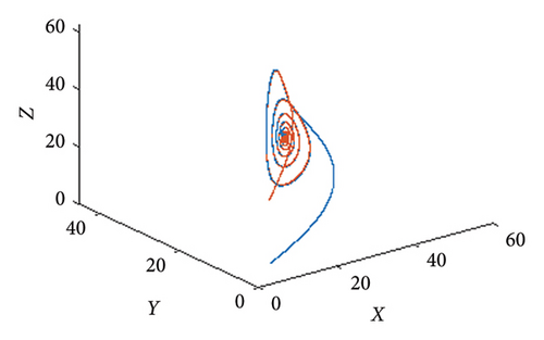
Let us increase the value b₁ to 1.2 and fix other parameter values as given in equation (105), then parameter values satisfy the GAS conditions for Prey Y-free steady state point, and Figure 2 confirms that.

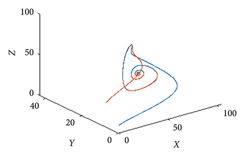
Again, let us increase the value b₂ to 1.1 and fix other parameter values as given in equation (105), then parameter values satisfy the GAS conditions for Prey X-free steady state point, and Figure 3 confirms that.

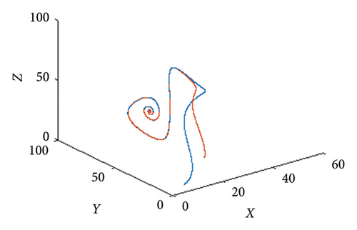
According to the fear level, it is observed the long-term behavior for a range of values f ∈ , in Figures 4, 5, and 6, and bifurcation diagram with respect to f is drawn. From Figure 4, all species show oscillatory for the small values of f. From Figure 5, the population of Prey X and predators show oscillatory for the further smaller values of f. From Figure 5, the population of Prey Y and predators show oscillatory for the further smaller values of f.

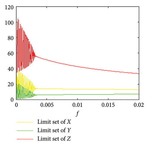
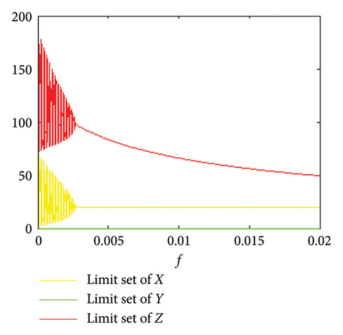
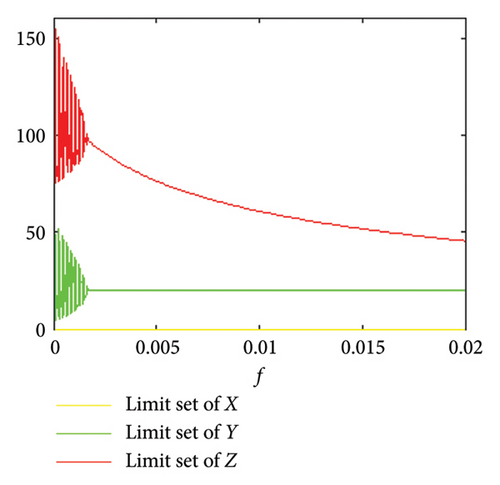
In general, Figures 4, 5, and 6 indicate that decreasing the fear level may induce a transition from the stability situation to the state where the populations oscillate periodically.

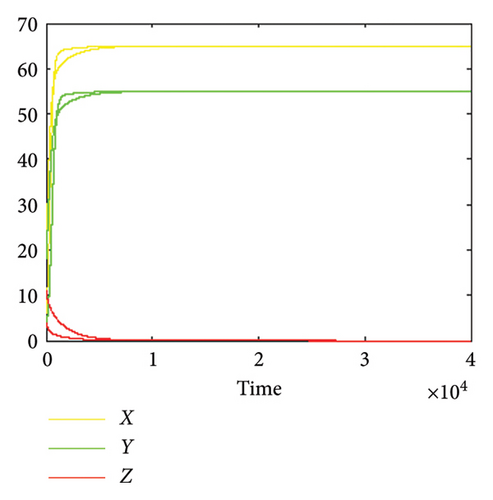
Let us increase the value of d to 0.3 and fix other parameter values given in equation (105), then λ_1Z become negative, which satisfy the stable condition for the predator free steady state point, and Figure 7 confirms that.

Let us solve System 1, when f ∈ [0, 10], d = 0.3, and other parameter values are fixed as given in equation (105), then the dynamics of system near predator free steady state point does not change; this confirms the theoretical result that the fear level has no impact on LAS of predator free equilibrium point; see Figure 8.

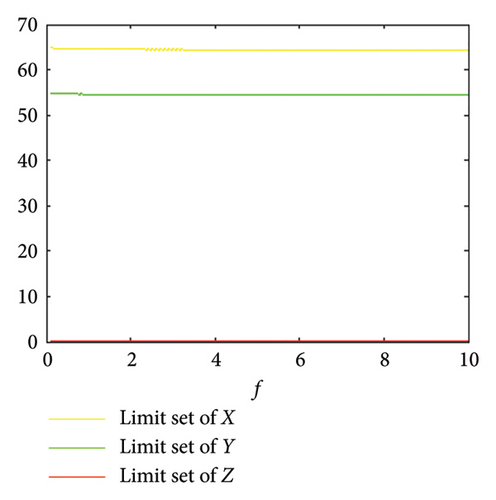
The above figure indicates that the fear level has no impact on the dynamics near predator free steady state point.

7. Conclusion and Discussion

In this paper, System 1 has been formulated, consisting of two prey species and one predator species, and it is taken to consideration the fear effect on both prey species. It is explored that System (1) has at most seven steady state points, and they are denoted by P_i, i = 0, 1, 2, 3, 4, 5, 6, in the criteria for local as well as global stability for each steady state. Local bifurcation such as trans critical, saddle-node, and pitchfork bifurcation near the steady states P_i, i = 0, 1, 2, 3, are studied. Also, bifurcating values of fear level of predators f for the occurrence of Hopf bifurcation in System (1) near prey X free, prey Y free, and coexistence steady state points are determined. Numerically, we have shown that if the value of fear level is decreased, then System (2) may induce a transition from the stability situation to the state where the populations oscillate periodically.

Conflicts of Interest

The authors declare no conflicts of interest.

Funding

We confirm that the Manuscript 9391001 received no external funding.

Open Research

Data Availability Statement

The data that support the findings of this study are available on request from the corresponding author.

References

1 Al-Darabsah I., Tang X., and Yuan Y., A Prey-Predator Model With Migrations and Delays, Discrete and Continuous Dynamical Systems—Series B. (2016) 21, no. 3, 737–761, https://doi.org/10.3934/dcdsb.2016.21.737, 2-s2.0-84959919485.
10.3934/dcdsb.2016.21.737
Web of Science® Google Scholar
2 Elettreby M. F., Two-Prey One-Predator Model, Chaos, Solitons & Fractals. (2009) 39, no. 5, 2018–2027, https://doi.org/10.1016/j.chaos.2007.06.058, 2-s2.0-64049094660.
10.1016/j.chaos.2007.06.058
Web of Science® Google Scholar
3 Arif G. E., Alebraheem J., and Yahia W. B., Dynamics of Predator-Prey Model Under Fluctuation Rescue Effect, Baghdad Science Journal. (2023) 20, 1742–1750, https://doi.org/10.21123/bsj.2023.6938.
10.21123/bsj.2023.6938
Web of Science® Google Scholar
4 Kamal B. B. and Mustafa A. M., Dynamical Analysis of a Three Species Food-Web Model With Extended Holling Type II Functional Response, European Journal of Pure and Applied Mathematics. (2025) 18, no. 1, https://doi.org/10.29020/nybg.ejpam.v18i1.5397.
10.29020/nybg.ejpam.v18i1.5397
Web of Science® Google Scholar
5 Mondal C., Kesh D., and Mukherjee D., Bifurcation and Global Stability of a Discrete Prey–Predator Model With Saturated Prey Refuge, Mathematical Methods in the Applied Sciences. (2023) 46, no. 17, 18354–18374, https://doi.org/10.1002/mma.9562.
10.1002/mma.9562
Web of Science® Google Scholar
6 Fatah S., Mustafa A., and Shilan A., Predator and N-Classes-Of-Prey Model Incorporating Extended Holling Type II Functional Response for N Different Prey Species, AIMS Mathematics. (2022) 8, 5779–5788, https://doi.org/10.3934/math.202329.
10.3934/math.2023291
Google Scholar
7 Holling C. S., Some Characteristics of Simple Types of Predation and Parasitism, The Canadian Entomologist. (1959) 91, no. 7, 385–398, https://doi.org/10.4039/Ent91385-7, 2-s2.0-84880026161.
10.4039/Ent91385-7
Google Scholar
8 Molla H., Rahman M. S., and Sarwardi S., Dynamics of a Predator-Prey Model With Holling Type II Functional Response Incorporating a Prey Refuge Depending on Both the Species, International Journal of Nonlinear Sciences and Numerical Stimulation. (2019) 20, 89–104, https://doi.org/10.1515/ijnsns-2017-0224, 2-s2.0-85057616676.
10.1515/ijnsns-2017-0224
Web of Science® Google Scholar
9 He M. and Zhong, Stability of Fear Effect Predator-Prey Model Mutual Interference or Group Defense, Journal of Biological Dynamics. (2022) 16, 480–498, https://doi.org/10.1080/17513758.2022.2091800.
10.1080/17513758.2022.2091800
PubMed Google Scholar
10 Hallam T. G. and Clark C. E., Non-Autonomous Logistic Equations as Models of Populations in a Deteriorating Environment, Journal of Theoretical Biology. (1981) 93, no. 2, 303–311, https://doi.org/10.1016/0022-5193(81)90106-5, 2-s2.0-0019845154.
10.1016/0022-5193(81)90106-5
Web of Science® Google Scholar
11 Xue Y., Chen F., Xie X., and Chen S., An Analysis of a Predator-Prey Model in Which Fear Reduces Prey Birth and Death Rates, AIMS Mathematics. (2024) 9, no. 5, 12906–12927, https://doi.org/10.3934/math.2024630.
10.3934/math.2024630
Web of Science® Google Scholar
12 Hassan K., Mustafa A., and Hama M., An Eco-Epidemiological Model Incorporating Harvesting Factors, Symmetry. (2021) 13, no. 11, https://doi.org/10.3390/sym13112179.
10.3390/sym13112179
Web of Science® Google Scholar
13 Zanette L. Y., White A. F., Allen M. C., and Clinchy M., Perceived Predation Risk Reduces the Number of Offspring Songbirds Produce Per Year, Science. (2011) 334, no. 6061, 1398–1401, https://doi.org/10.1126/science.1210908, 2-s2.0-83255164813.
10.1126/science.1210908
CAS PubMed Web of Science® Google Scholar
14 Wang X., Zanette L., and Xinfu Zou X., Modeling the Fear Effect in Predator-Prey Interactions, Mathematical Biosciences. (2016) 73, 1–38, https://doi.org/10.1007/s00285-016-0989-1, 2-s2.0-84961843555.
10.1016/j.mbs.2016.01.005
CAS Google Scholar
15 Pal S., Pal N., Samanta S., and Chattopadhyay J., Effect of Hunting Cooperation and Fear in a Predator-Prey Model, Ecological Complexity. (2019) 39, https://doi.org/10.1016/j.ecocom.2019.100770, 2-s2.0-85067917048.
10.1016/j.ecocom.2019.100770
Web of Science® Google Scholar
16 Zhang H., Cay Y., Fu S., and Wang W., Impact of the Fear Effect in a Prey-Predator Model Incorporatingapreyrefuge, Applied Mathematics and Computation. (2019) 356, 328–337, https://doi.org/10.1016/j.amc.2019.03.034, 2-s2.0-85063610028.
10.1016/j.amc.2019.03.034
Google Scholar
17 Cong P., Fan M., and Xingfu Z., Dynamics of a Three-Species Food Chain Model With Fear Effect, Communications in Nonlinear Science and Numerical Simulation. (2021) 99, https://doi.org/10.1016/j.cnsns.2021.105809.
10.1016/j.cnsns.2021.105809
Web of Science® Google Scholar
18 Tan Y., Cai Y., Yao R., Hu M., and Wang W., Complex Dynamics in an Eco-Epidemiological Model With the Cost of Anti-predator Behaviors, Nonlinear Dynamics. (2022) 107, no. 3, 3127–3141, https://doi.org/10.1007/s11071-021-07133-4.
10.1007/s11071-021-07133-4
Web of Science® Google Scholar
19 Jimil A. R. and Naji R. K., Modeling and Analyzing the Influence of Fear on the Harvested Modified Leslie Gower Model, Baghdad Science Journal. (2023) 20, no. 5, 1701–1712.
Google Scholar
20 Pal S., Tiwari P. K., Misra A. K., and Wang H., Fear Effect in a Three-Species Food Chain Model With Generalist Predator, Mathematical Biosciences and Engineering. (2023) 21, 1–33, https://doi.org/10.3934/mbe.2024001.
10.3934/mbe.2024001
Google Scholar
21 liu J., Lv P., Liu B., and Zhang T., Dynamics of a Predator-Prey Model With Fear Effect and Time Delay, Complexity (New York, N. Y.). (2021) 2021, no. 1, https://doi.org/10.1155/2021/9184193.
10.1155/2021/9184193
Google Scholar
22 Mohammed H. A. and Mustafa A. N., Dynamical Analysis of a Delay Two-Prey–One-Predator Model Incorporating Fear Effect in the Growth Rate of Preys, Journal of Applied Mathematics. (2025) 2025, no. 1, https://doi.org/10.1155/jama/5535248.
10.1155/jama/5535248
Web of Science® Google Scholar

All articles

Local Bifurcation and Global Stability of Two-Prey-One-Predator Model

Abstract

1. Introduction

1.1. Motivation and Literature Survey

1.2. The Model Formulation

1.3. Problem Statement and Key Contribution

1.4. Layout of the Paper

2. Positivity and Boundedness

3. Existence of Steady State Points

4. Local Stability and Local Bifurcation

5. Global Stability

6. Numerical Simulation

7. Conclusion and Discussion

Conflicts of Interest

Funding

Open Research

Data Availability Statement

References

Figures

References

Information

About Wiley Online Library

Help & Support

Opportunities

Connect with Wiley

Local Bifurcation and Global Stability of Two-Prey-One-Predator Model

Abstract

1. Introduction

1.1. Motivation and Literature Survey

1.2. The Model Formulation

1.3. Problem Statement and Key Contribution

1.4. Layout of the Paper

2. Positivity and Boundedness

3. Existence of Steady State Points

4. Local Stability and Local Bifurcation

5. Global Stability

6. Numerical Simulation

7. Conclusion and Discussion

Conflicts of Interest

Funding

Open Research

Data Availability Statement

References

Figures

References

Related

Information