A Comparative Study of Linearization Techniques With Adaptive Block Hybrid Method for Solving First-Order Initial Value Problems
Abstract
This paper investigates linearization methods used in the development of an adaptive block hybrid method for solving first-order initial value problems. The study focuses on Picard, linear partition, simple iteration, and quasi-linearization methods, emphasizing their role in enhancing the performance of the adaptive block hybrid method. The efficiency and accuracy of these techniques are evaluated through solving nonlinear differential equations. The study provides a comparative analysis focusing on convergence properties, computational cost, and the ease of implementation. Nonlinear differential equations are solved using the adaptive block hybrid method, and for each linearization method, we determine the absolute error, maximum absolute error, and number of iterations per block for different initial step-sizes and tolerance values. The findings indicate that the four techniques demonstrated absolute errors, ranging from O(10−12) to O(10−20). We noted that both the Picard and quasi-linearization methods consistently achieve the highest accuracy in minimizing absolute errors and enhancing computational efficiency. Additionally, the quasi-linearization method required the fewest number of iterations per block to achieve its accuracy. Furthermore, the simple iteration method required fewer number of iterations than the linear partition method. Comparing minimal CPU time, the Picard method required the least. These results address a critical gap in optimizing linearization techniques for the adaptive block hybrid method, offering valuable insights that enhance the precision and efficiency of methods for solving nonlinear differential equations.
1. Introduction
Nonlinear differential equations arise in various fields of science and engineering, and obtaining accurate solutions to these problems remain a challenging task to researchers. Numerical methods are essential for solving nonlinear differential equations that lack analytical solutions [1]. Many numerical methods allow for iterative refinement and visualization of solutions, making them valuable for practical applications in science and engineering [2].
Block hybrid methods (BHMs) have emerged as promising numerical methods, combining the strengths of multistep and one-step methods to provide efficient and stable numerical schemes [3]. It is widely recognized that BHMs are capable of efficiently solving initial value problems (IVPs) and boundary value problems (BVPs) [4, 5]. The theoretical properties of the BHM, such as convergence order, zero-stability, and consistency, to ensure their convergence have been investigated [6]. Many researchers are focusing on improving BHM to enhance the efficiency and convergence when solving differential equations [7, 8]. The goal is to develop more accurate and robust BHMs that can handle a wider range of problems, including nonlinear IVPs. For example, some of the key areas being explored include deriving new k-step hybrid block methods with higher orders of accuracy and better stability properties [9]. Other innovations include incorporating off-grid points within the block to improve the approximation solutions [10] and employing different basis functions, such as Hermite polynomials, to construct the continuous linear multistep methods that form the foundation of the BHM [11]. Focusing on these aspects, researchers aim to develop BHMs that are not only more accurate but are also computationally efficient and reliable for solving differential equations.
One technique used to improve the BHM is to utilize variable step-sizes instead of a fixed step-size scheme [12]. This adaptive technique offers several advantages, such as improving the accuracy of the solution by adjusting the step-size to achieve the desired level of precision without wasting computational time or introducing unnecessary errors [13]. Adaptive techniques can enhance the efficiency of the method by avoiding unnecessary evaluations of the function or its derivatives, and thereby saving time and memory [14]. The variable step-size scheme can improve the stability of the method by using smaller step-sizes when needed to avoid numerical instability or divergence that may occur with a fixed step-size approach [15]. There are several existing methods for introducing adaptivity in numerical methods [16]. One such technique is the use of embedded methods that use two approximations of different orders at each step, and the difference is taken as an estimate of the local error [17, 18]. Examples of these include the Runge–Kutta–Fehlberg method, the Dormand–Prince method, and the Cash–Karp method [19–21].
Several researchers have investigated different strategies for implementing the adaptive block hybrid method (ABHM) for solving nonlinear differential equations [22]. Some ABHMs employ two different approximations, each of a different order of accuracy, at each step [23]. The difference between these two approximations is then used as a local error estimate at that step. This error estimates the key that allows the method to adaptively adjust the step-size to maintain a desired accuracy in the computation [24]. Singh et al. [23] presented an efficient optimized adaptive hybrid block method for IVPs. The authors utilized three off-step points within the one-step block. Two of the off-step points were optimized to minimize the local truncation errors (LTEs) of the main method. The adaptive method was tested on several well-known systems and it compared favorably with other numerical methods in the literature. Rufai et al. [25] proposed an adaptive hybrid block method for solving first-order IVPs of ordinary differential equations and partial differential equation problems. The method was formulated in a variable step-size and implemented with an adaptive step-size strategy to maintain the error within a specified tolerance. It was demonstrated that the method was more efficient than some other existing numerical methods used in solving the differential equations in the study.
A key aspect of enhancing the accuracy of a numerical approximation is the choice of the linearization technique [26]. Linearization is necessary to transform the nonlinear problem into a form that can be easily solved [27]. Linearization methods are therefore important for the purpose of transforming nonlinear differential equations into linear equations that are easier to solve using numerical techniques [28]. The choice of the linearization method can impact the stability of the numerical scheme, its accuracy, and computational efficiency [29]. Some well-known linearization techniques include the Taylor series linearization which involves expanding the nonlinear function in a Taylor series around a point of interest and truncating higher-order terms. This is straightforward but may require small step-sizes for accuracy [30]. Newton’s method uses an iterative technique where the nonlinear equation is approximated by a linear one at each iteration step [31]. It is highly accurate but can be computationally intensive [32].
- •
What are the existing linearization methods used with ABHM, and what are their strengths and weaknesses?
- •
How can linearization techniques be implemented with the ABHM, and how does the performance compare with other numerical methods?
The Picard method (PM) is based on the Picard–Lindelöf theorem, which ensures the existence and uniqueness of solutions for IVPs [34–36]. The PM starts with an initial guess which is then refined iteratively by integrating the nonlinear function over the interval of interest [37, 38]. The PM is a straightforward method that may however not always converge as it relies on the assumption that the nonlinear function is locally Lipschitz continuous, which is not always the case [39]. The PM converges linearly, meaning that the error in the solution decreases at a constant rate [40]. This can lead to a slow convergence rate, especially for problems with complex nonlinearities. The PM was utilized with the BHM to solve second-order IVPs by Rufai et al. [9].
There are several local and piece-wise linearization schemes for IVPs, the use of which depend on the algorithm employed in the numerical implementation [41–44]. The piece-wise linearization approach is useful for handling nonlinearities locally, making the overall problem more tractable [45]. The linear partition method (LPM) linearization scheme is a modified piece-wise linearization approach that allows for flexibility in handling the nonlinearities [46]. The LPM is a direct scheme and is particularly useful for solving stiff differential equations. The LPM used to linearize first-order IVPs and combined with the BHM by Shateyi [5]. Similarly, the simple iteration method (SIM) technique is a piece-wise linearization approach that is easy to implement and is very effective for IVPs [47]. Ahmedai Abd Allah et al. [47] proposed a SIM and used it with the BHM to solve third-order IVPs. The SIM works similar to fixed-point iteration [48].
The quasi-linearization method (QLM) transforms the nonlinear equations into a sequence of linear problems [49]. This method is similar to Newton’s method for root-finding but applied to differential equations [50]. At each iteration, the method linearized the nonlinear terms around the current solution estimate, resulting in a linear differential equation that can be solved to update the solution. The QLM converges quadratically, making it very efficient for problems where a good initial guess is available [51]. It is particularly effective for strongly nonlinear problems where other linearization methods might not converge [52]. Motsa [53] implemented the BHM with the QLM to solve first-order IVPs.
2. Implementation of the BHM
3. Theoretical Analysis
In this section, we investigate the order, error constant, linear stability, order star, and zero stability analysis of the BHM.
3.1. LTE and Consistency
Comparing equations (18) and (20) yields q = m + 1 as the order of the BHM. Following [56, 57], a block method is consistent if its order q ≥ 1. This condition is satisfied since m ≥ 2.
3.2. Zero Stability and Convergence
The roots of the characteristic equation, called the characteristic roots, must satisfy all roots of ρ(λ) ≤ 1. Furthermore, any roots must have multiplicity one. This ensures that the method is zero stable, which is a prerequisite for convergence. Hence, the BHMs developed in this study are zero-stable. Since these methods exhibit both zero-stability and consistency, Dahlquist’s theorem implies that they are convergent [54].
3.3. Absolute Stability
| m | pj | Stability function |
|---|---|---|
| 2 | 0, (1/2), 1 | (24 − z2)/(2(z2 − 6z + 12)) |
| 3 | 0, (1/3), (2/3), 1 | (−z3 + 3z2 + 54z − 324)/(3(z3 − 11z2 + 54z − 108)) |
| 4 | 0, (1/4), (1/2), (3/4), 1 | (−3z4 + 20z3 + 240z2 − 3840z + 15360)/(4(3z4 − 50z3 + 420z2 − 1920z + 3840)) |
| 5 | 0, (1/5), (2/5), (3/5), (4/5), 1 | (−12z5 + 130z4 + 1125z3 − 37500z2 + 337500z − 1125000)/(5(12z5 − 274z4 + 3375z3 − 25500z2 + 112500z − 225000)) |
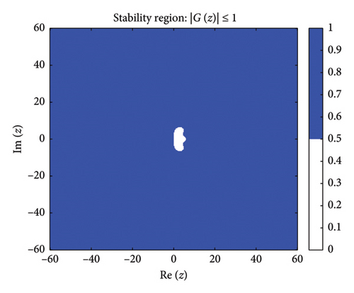
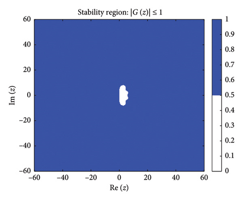
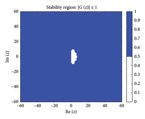
Figure 1 shows the absolute stability regions of the BHM for different values of (m = 2, 3, 4, 5). The shaded areas represent the set of complex values z = hλ where the stability condition is satisfied.

Definition: Following [63], a numerical method for solving ordinary differential equations is A-stable if its region of absolute stability contains the entire left half-plane of .
Figure 1 shows the absolute stability regions for m = 2, 3, 4, 5, confirming the A-stability of the BHM as the entire left-half complex plane is covered.
- 1.
Its region of absolute stability contains the entire left half-plane.
- 2.
Its stability function satisfies
() -
From Table 1, we compute the asymptotic behavior of each stability function as z⟶∞, which yields
() -
Since none of the stability functions satisfy , the BHM is not L-stable for any m ≥ 2, despite being A-stable (as shown in Figure 1).
3.4. Order Stars
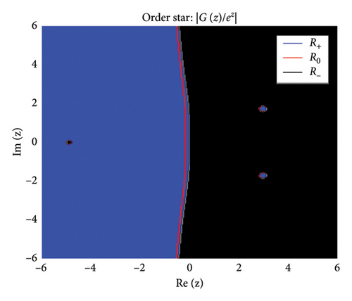
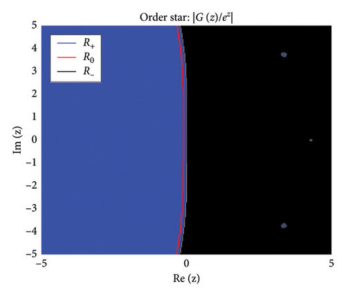
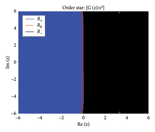
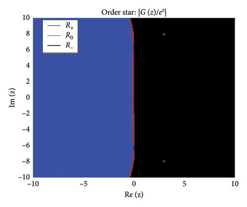
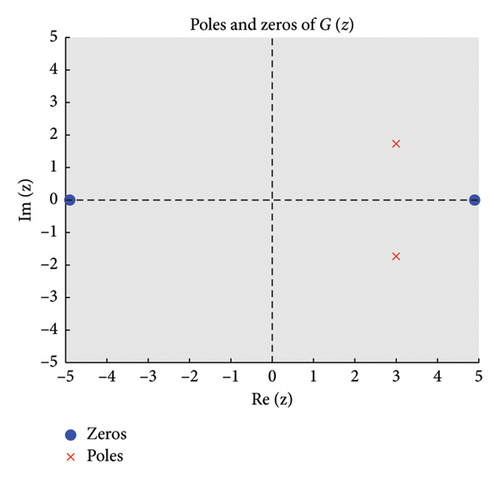
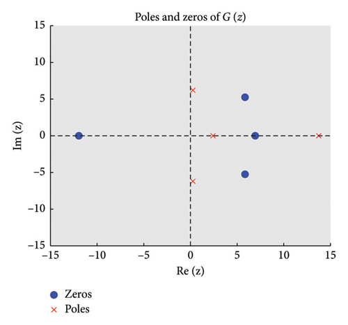
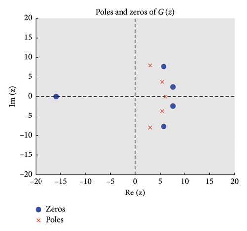
The zeros of (roots of ) appear as points where stable regions contract, indicating strong damping properties, while poles (roots of ) act as sources of instability where unstable regions diverge. Figures 2 and 3 show the structure of the three regions, zeros, and poles of the BHM, respectively.

- •
The growth region R+ does not intersect the imaginary axis.
- •
There are no poles of in the left half of the complex plane, i.e., Re(z) < 0.
These conditions ensure that the numerical method exhibits stable behavior. Figure 2 shows the order stars stability region for the scheme. It is observed that the region contains the entire left half of the complex plane for all values of (m = 2, 3, 4, 5). It is also noted that R+ does not intersect the imaginary axis, and no poles are found in the left of the complex plane (as shown in Figure 3). Thus, we conclude that the method is A-acceptable.
4. The Adaptive Scheme
In this case, the LTE from equation (18) are given in Table 2.
| pj | p1 | p2 | p3 | p4 | p5 |
|---|---|---|---|---|---|
| Local truncation error | −(863y(7)(tr)h7)/4725000000 | −(37y(7)(tr)h7)/295312500 | −(29y(7)(tr)h7)/175000000 | −(8y(7)(tr)h7)/73828125 | −(11y(7)(tr)h7)/37800000 |
An adaptive counterpart of the main method yr+1 can be constructed utilizing the method of undetermined coefficients on an equation with identical grid points, except at p5 = 1. This expression has a LTE in Table 3.
| pj | p1 | p2 | p3 | p4 | p5 |
|---|---|---|---|---|---|
| Local truncation error | (3y(6)(tr)h6)/2500000 | (y(6)(tr)h6)/1406250 | (3y(6)(tr)h6)/25000000 | −(8y(7)(tr)h7)/73828125 | (19y(6)(tr)h6)/900000 |
- •
If ‖EST‖ < Tol1, we accept the procured values and increase the step-size by hnew = 2hold, to forward the integration process.
- •
If ‖EST‖ ≥ Tol1, we recalibrate the current step-size employing the criterion in equation (38) and recalculate.
By the above methodology, we ensure a reliable error estimation and optimize the step-size for each integration block in the ABHM.
4.1. Error Estimation
This provides a measure of how much the solution changes between iterations, indicating the convergence behavior of the method.
We evaluate in Algorithm 1 the following conditional stopping procedure in the ABHM where Tol2 represents the second user-defined tolerance. Within each block, the method iterates until the error AEE falls below Tol2. Once the AEE converges to within an acceptable criteria, the procedure advances to the next block or concludes the computation. By applying this conditional structure, we ensure that the accuracy of our solutions is systematically improved within each block, thereby enhancing control and precision in the numerical computations. The pseudo-code loops through the steps until convergence or the maximum number of iterations is reached.
-
Algorithm 1: ABHM algorithm pseudo-code.
-
Step 1: Input IVP f(t, y), tolerance levels Tol1, Tol2, initial step-size h0, safety factor σ, and max iterations.
-
Step 2: Initialize Yr+p, Fr+p, Yr, Fr.
-
Step 3: While not converged (AEE < Tol2) or max iterations not reached, do Steps 4–11:
-
Step 4: Compute using the ABHM equation.
-
Step 5: Compute yr+1 and using adaptive pair equations.
-
Step 6: Compute the error estimate EST,
-
if‖EST‖ < Tol1then
-
(a) Accept the current .
-
(b) Set hnew = 2 × hold.
-
else
-
(c) Set .
-
end if
-
Step 10: Update Yr+p and Fr+p with hnew.
-
Step 11: Update hold to hnew.
-
Step 12: Return Yr+p.
5. Linearization Techniques
In this section, we discuss various linearization approaches, namely, PM, LPM, SIM, and QLM, that must be applied to linearized equation (1) before using ABHM equation (10). ABHM equation (10) is a powerful numerical approach for solving differential equations, offering accuracy and efficiency by adapting to the problem’s behavior. However, the nonlinear nature of many IVPs necessitates an initial linearization step to facilitate the application of the ABHM. These techniques transform nonlinear IVPs into linear equations, which are easier to solve. Consider that f is a nonlinear function and F is the linearized form of f. The linear and nonlinear terms are evaluated as known and unknown terms at iteration s and s + 1, respectively.
5.1. PM
Equation (43) represents the Picard adaptive block hybrid method (PM-ABHM) equations.
5.2. LPM
5.3. SIM
5.4. QLM
6. Numerical Results and Discussion
In this section, we present and analyze the numerical results obtained by implementing the ABHM on various first-order IVPs with particular focus on demonstrating the effectiveness and accuracy of the adaptive BHM, particularly when utilizing several linearization schemes in the case m = 5 and σ = 0.9. All computational experiments have been performed using MATLAB R2021b.
6.1. Example 1
- •
PM: .
- •
LPM: .
- •
SIM: .
- •
QLM: .
Figure 4 shows the numerical and exact solutions for equation (60). It can be observed that the approximate and exact solutions coincide.
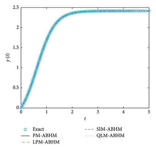
Figure 5 shows the AE for different linearization techniques with varying initial step-sizes and the first user-defined tolerance. As shown in Figure 5(a), the PM-ABHM, LPM-ABHM, SIM-ABHM, and QLM-ABHM achieve an AE ranging from O(10−13) to O(10−17) for h0 = 10−1 and Tol1 = 10−8. Figure 5(b) presents the AE for these methods with h0 = 10−2 and Tol1 = 10−10, where all methods maintain an AE between O(10−13) and O(10−19).

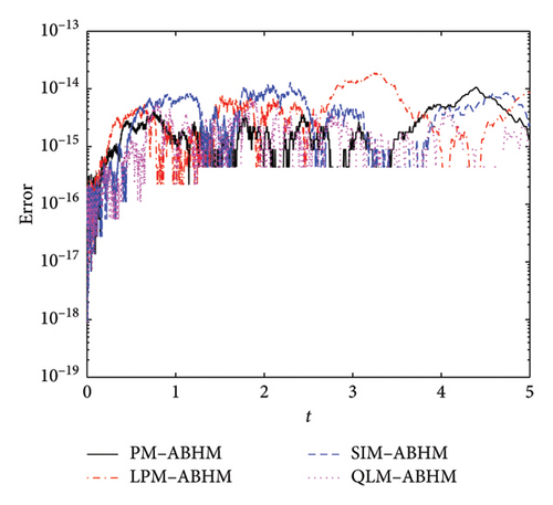
Table 4 compares the maximum AE for different linearization schemes of the ABHM at Tol2 = 10−13 with varying h0 and Tol1. From Table 4, it is evident that the PM-ABHM, SIM-ABHM, and QLM-ABHM achieve a maximum AE of order O(10−15), while the LPM-ABHM records a maximum AE of order O(10−14) for h0 = 10−1 and Tol1 = 10−8. For h0 = 10−2 and Tol1 = 10−10, QLM-ABHM maintains a maximum AE of order O(10−15), while the PM-ABHM, LPM-ABHM, and SIM-ABHM achieve a maximum AE of order O(10−14). The results show that QLM-ABHM outperforms the other methods, with LPM-ABHM having the highest maximum AE. Table 4 reveals that PM-ABHM is the fastest for both h0 = 10−1 and h0 = 10−2.
| tF | h0 | Tol2 | PM-ABHM | LPM-ABHM | SIM-ABHM | QLM-ABHM |
|---|---|---|---|---|---|---|
| 5 | 10−1 | 10−8 | 6.2172 × 10⁻¹⁵ | 1.5543 × 10⁻¹⁴ | 6.6613 × 10⁻¹⁵ | 5.3291 × 10⁻¹⁵ |
| CPU time in seconds | 0.012192 | 0.082196 | 0.088391 | 0.052143 | ||
| 5 | 10−2 | 10−10 | 1.0658 × 10⁻¹⁴ | 1.8652 × 10⁻¹⁴ | 1.2879 × 10⁻¹⁴ | 6.6613 × 10⁻¹⁵ |
| CPU time in seconds | 0.061403 | 0.255753 | 0.263201 | 0.189779 | ||
Figure 6 shows the number of iterations per block for different linearization schemes with varying initial step-sizes and the first user-defined tolerance. Figure 6(a) illustrates the performance of the PM, LPM, SIM, and QLM schemes for h0 = 10−1 and Tol1 = 10−8. We observe that the maximum number of iterations required is 10 for LPM-ABHM, while the PM-ABHM and SIM-ABHM schemes require a maximum of eight iterations, and QLM-ABHM requires between three to four iterations. As shown in Figure 6(b), for smaller initial step-sizes and the first user-defined tolerance, the number of iterations per block is reduced to seven for LPM-ABHM. However, the PM-ABHM and SIM-ABHM schemes decrease to six iterations, while QLM-ABHM decreases to between two to three iterations. This indicates that smaller initial step-sizes and the first user-defined tolerance decrease the number of iterations per block, leading to rapid convergence of the ABHM.

6.2. Example 2
- •
PM: .
- •
LPM: .
- •
SIM: .
- •
QLM: .
Figure 7 depicts the numerical and exact solution using PM-ABHM, LPM-ABHM, SIM-ABHM, and QLM-ABHM, respectively. We note that the numerical solutions match the exact solution.
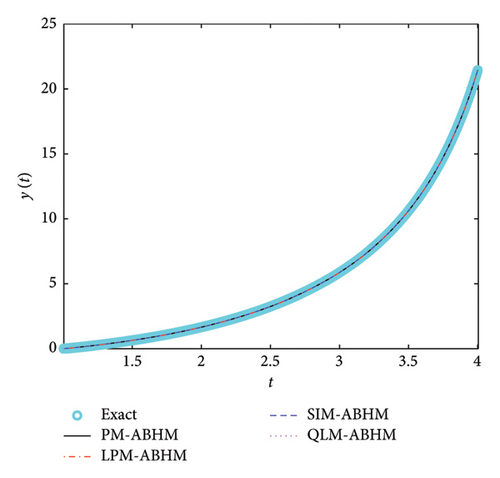
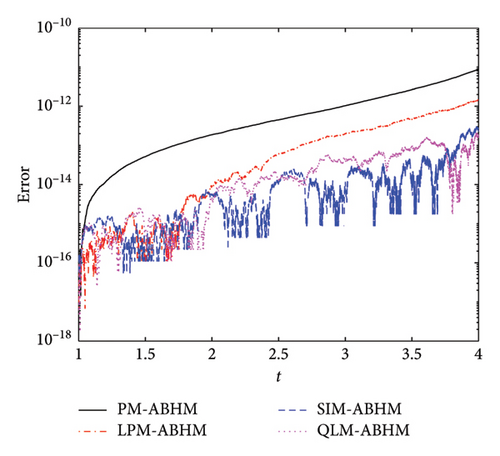
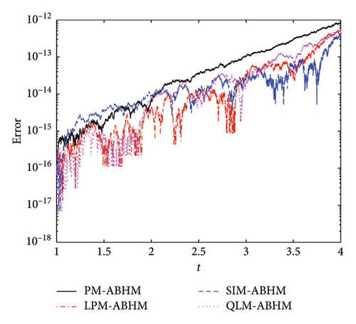
Figure 8 and Table 5 present a comparison of the AE and the maximum AE achieved using the PM-ABHM, LPM-ABHM, SIM-ABHM, and QLM-ABHM, respectively, for different initial step-sizes and second user-defined tolerances. Figure 8(a) shows that for h0 = 10−1 and Tol2 = 10−12, all methods achieve an AE between O(10−11) and O(10−17). Similarly, Figure 8(b) shows that for h0 = 10−3 and Tol2 = 10−14, the AE ranges from O(10−12) to O(10−17). These results indicate that smaller initial step-sizes and second user-defined tolerances lead to higher precision.
| tF | h0 | Tol2 | PM-ABHM | LPM-ABHM | SIM-ABHM | QLM-ABHM |
|---|---|---|---|---|---|---|
| 4 | 10−1 | 10−12 | 8.8143 × 10⁻¹² | 1.4779 × 10⁻¹² | 3.0198 × 10⁻¹³ | 2.1672 × 10⁻¹³ |
| CPU time in seconds | 0.079389 | 0.408207 | 0.362927 | 0.309272 | ||
| 4 | 10−3 | 10−14 | 8.5620 × 10⁻¹³ | 5.0449 × 10⁻¹³ | 4.2633 × 10⁻¹³ | 5.4001 × 10⁻¹³ |
| CPU time in seconds | 0.121848 | 0.467590 | 0.447170 | 0.297296 | ||
From Table 5, it is evident that the maximum AE improves with smaller h0 and Tol2 for all methods, although the improvement is marginal. Regarding CPU time, the PM-ABHM and QLM-ABHM are faster compared to the LPM-ABHM and SIM-ABHM.
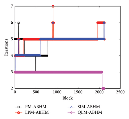
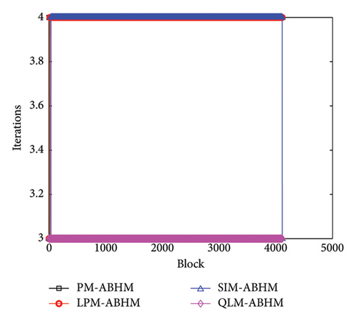
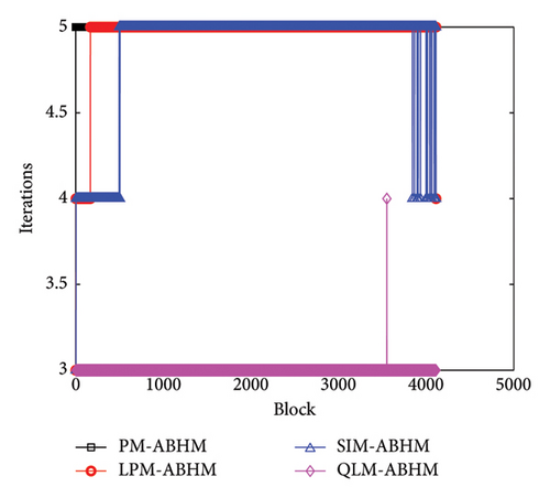
Figure 9 compares the number of iterations per block required for all methods with varying h0 and Tol2. Figure 9(a) shows the performance of the PM, LPM, SIM, and QLM for h0 = 10−1 and Tol2 = 10−12. We observe that the maximum number of iterations required is four for PM-ABHM, while LPM-ABHM and SIM-ABHM require between three and four iterations, and the QLM-ABHM scheme requires three iterations. As shown in Figure 9(b), when h0 = 10−3 and Tol2 = 10−14, the number of iterations increases by one for all methods.
6.3. Example 3
- •
PM: .
- •
LPM: .
- •
SIM: .
- •
QLM: .
In Figure 10, the numerical and exact solutions for Example 3 are presented using PM-ABHM, LPM-ABHM, SIM-ABHM, and QLM-ABHM, respectively. It is evident from Figure 10 that the approximate solutions match the exact solutions.
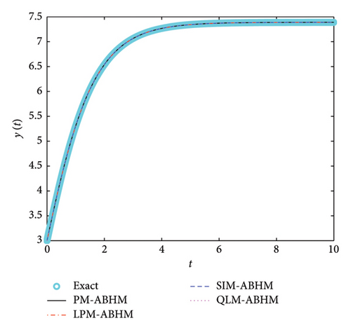
Figure 11 presents the AE for the four techniques for different values of the second user-defined tolerance. Figures 11(a) and 11(b) show that the AE for PM-ABHM, LPM-ABHM, SIM-ABHM, and QLM-ABHM is less than or equal to O(10−13) for Tol2 = 10−12 and Tol2 = 10−14, respectively. It can be observed that for the same initial step-size but different Tol2, the AE remains within the same order.
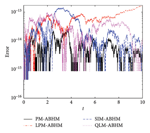
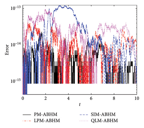
Table 6 compares the maximum AEs for the ABHMs. For Tol2 = 10−12, PM-ABHM and QLM-ABHM achieve O(10−14) error, while LPM-ABHM and SIM-ABHM have O(10−13). For Tol2 = 10−14, all methods except SIM-ABHM achieve O(10−14). The PM-ABHM and QLM-ABHM are faster than LPM-ABHM and SIM-ABHM.
| tF | h0 | Tol2 | PM-ABHM | LPM-ABHM | SIM-ABHM | QLM-ABHM |
|---|---|---|---|---|---|---|
| 10 | 10−2 | 10−12 | 2.4869 × 10⁻¹⁴ | 1.7408 × 10⁻¹³ | 1.4477 × 10⁻¹³ | 9.5923 × 10⁻¹⁴ |
| CPU time in seconds | 0.303831 | 1.071535 | 1.089501 | 0.917177 | ||
| 10 | 10−2 | 10−14 | 2.3093 × 10⁻¹⁴ | 4.1744 × 10⁻¹⁴ | 1.2434 × 10⁻¹³ | 9.5923 × 10⁻¹⁴ |
| CPU time in seconds | 0.324150 | 1.252072 | 1.112535 | 0.979220 | ||
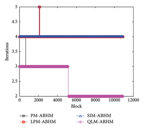
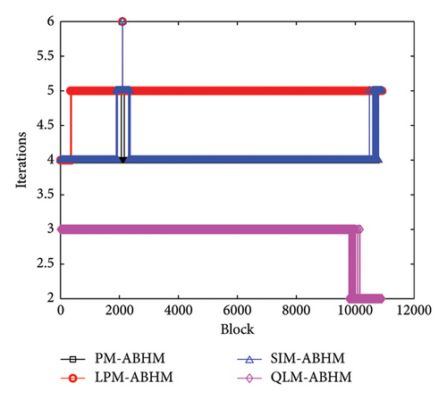
Figure 12 shows the number of iterations per block using PM-ABHM, LPM-ABHM, SIM-ABHM, and QLM-ABHM for different values of Tol2. In Figure 12(a), the PM requires between three and four iterations, while LPM-ABHM and SIM-ABHM require between four and five iterations, and QLM-ABHM requires between two and three iterations for Tol2 = 10−12. In Figure 12(b), for Tol2 = 10−14, the number of iterations for PM-ABHM, LPM-ABHM, and SIM-ABHM increases by one, while QLM-ABHM maintains the same number of iterations.
6.4. Example 4
- •
PM: .
- •
LPM: .
- •
SIM: .
- •
QLM: .
We depicted the exact and numerical solutions for Example 4 in Figure 13. It is evident that the numerical solutions closely align with the exact solution.
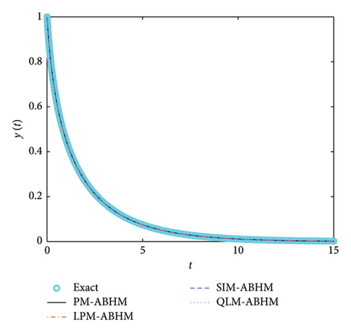
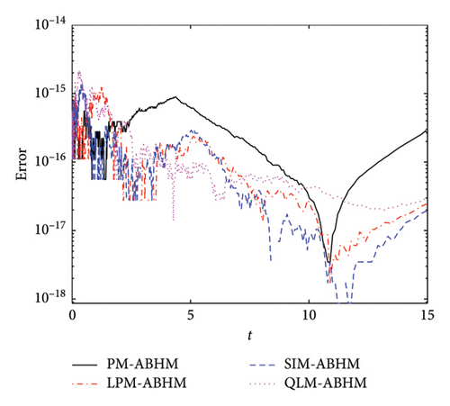
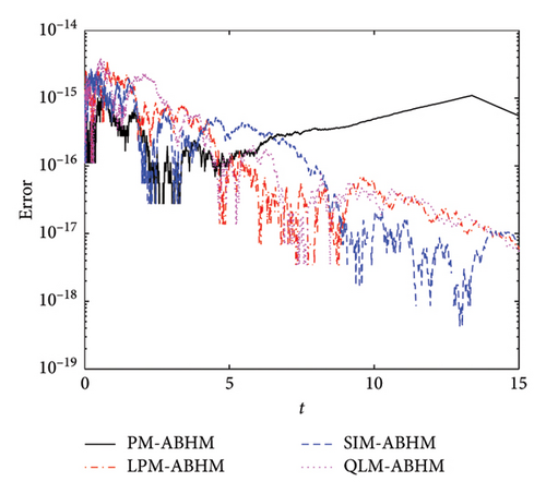
Figure 14 presents the AE for the PM-ABHM, LPM-ABHM, SIM-ABHM, and QLM-ABHM with varying initial step-sizes and the first user-defined tolerance. Figure 14(a) shows that the AE for these methods ranges from O(10−14) to O(10−18) for h0 = 10−1 and Tol1 = 10−8. In Figure 14(b), the AE for all four methods ranges from O(10−14) to O(10−19). We noted that smaller initial step-sizes and the first user-defined tolerance result in improved AE.
A comparison of the maximum AEs is shown in Table 7. The PM-ABHM achieves a maximum AE of O(10−16), while the LPM-ABHM, SIM-ABHM, and QLM-ABHM achieve maximum errors of O(10−15) for h0 = 10−1 and Tol1 = 10−8. For h0 = 10−3 and Tol1 = 10−10, all methods reach a maximum AE of O(10−15). The PM-ABHM consistently provides the smallest maximum AE across varying initial step-sizes and first user-defined tolerances, demonstrating its superior accuracy. The CPU times for each method differ, with PM-ABHM being the fastest.
| tF | h0 | Tol1 | PM-ABHM | LPM-ABHM | SIM-ABHM | QLM-ABHM |
|---|---|---|---|---|---|---|
| 15 | 10−1 | 10−8 | 8.8818 × 10⁻¹⁶ | 1.2768 × 10⁻¹⁵ | 1.3323 × 10⁻¹⁵ | 2.2204 × 10⁻¹⁵ |
| CPU time in seconds | 0.048587 | 0.129061 | 0.114315 | 0.071829 | ||
| 15 | 10−3 | 10−10 | 1.3323 × 10⁻¹⁵ | 3.3307 × 10⁻¹⁵ | 2.6645 × 10⁻¹⁵ | 3.7748 × 10⁻¹⁵ |
| CPU time in seconds | 0.131735 | 0.388458 | 0.396925 | 0.297469 | ||
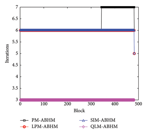
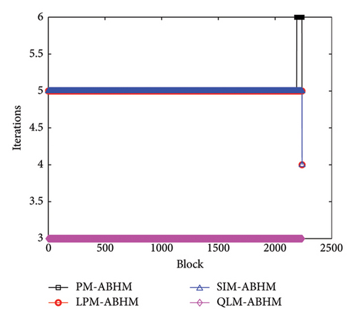
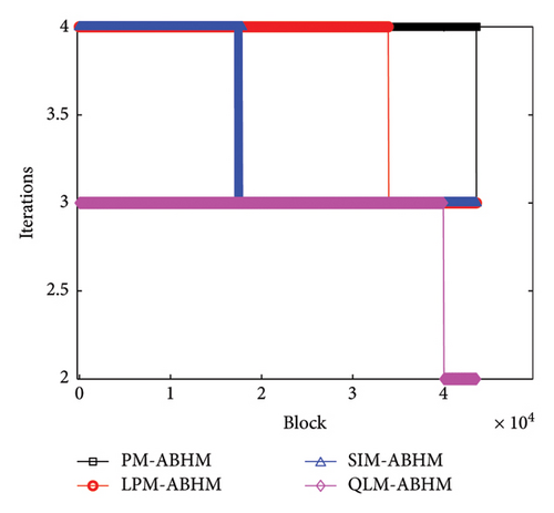
Figure 15 shows the number of iterations per block for the four methods with different initial step-sizes and first user-defined tolerance values. In Figure 15(a), the PM-ABHM requires six to seven iterations, while LPM-ABHM and SIM-ABHM need five to six, and QLM-ABHM only three iterations per block for h0 = 10−1 and Tol1 = 10−8. For h0 = 10−3 and Tol1 = 10−10, as shown in Figure 15(b), the number of iterations decreases by one for PM-ABHM, LPM-ABHM, and SIM-ABHM, while QLM-ABHM requires only three iterations.
6.5. Example 5
- •
PM: .
- •
LPM: .
- •
SIM: .
- •
QLM: .
We present the numerical and exact solutions in Figure 16. Figure 16 shows that the graphs of the approximate and exact solutions coincide.
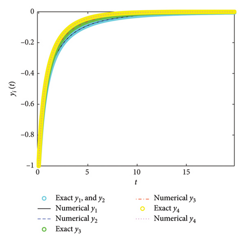
Figure 17 presents a comparative analysis of the AEs for the four implemented methods. We used h0 = 10−2, Tol1 = 10−12, Tol2 = 10−12, and tF = 20. Figure 17(a) illustrates the AE for the PM-ABHM. The PM demonstrates a high initial error O(10−14) that decreases consistently, achieving errors as low as O(10−20). Figure 17(b) depicts the AE for the LPM-ABHM. The LPM shows a similar trend of error reduction over time. The LPM-ABHM achieves errors in the range of O(10−13) to O(10−17). Figure 17(c) shows the AE for the SIM-ABHM. The SIM scheme manages to reduce the errors reaching O(10−18). Figure 17(d) presents the AE for the QLM-ABHM. The QLM technique shows a more consistent reduction in errors compared to the SIM. The error graphs decrease, reaching values between O(10−13) and O(10−19). It is evident that all four methods are capable of achieving low AEs.
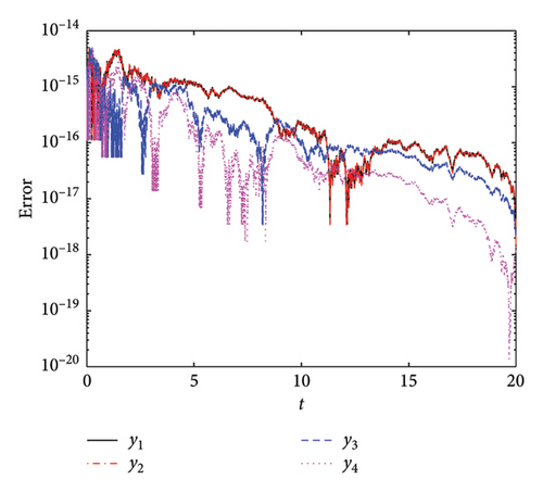
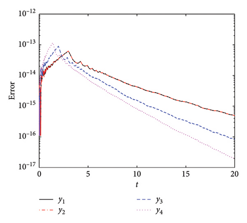
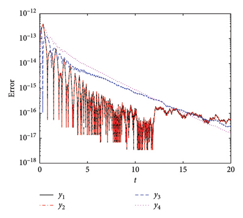
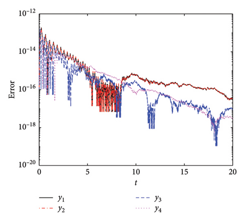
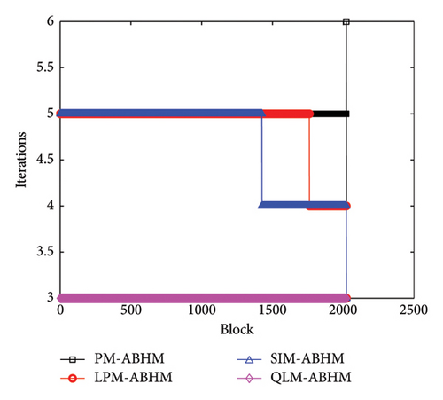
Figure 18 illustrates the number of iterations per block for the PM-ABHM, LPM-ABHM, SIM-ABHM, and QLM-ABHM at various Tol1 values in Example 5. In Figure 18(a), for Tol1 = 10−10, the PM-ABHM required five to six iterations per block, while the LPM-ABHM and SIM-ABHM maintained around four and five iterations, respectively. The QLM-ABHM consistently performs better, requiring only three iterations. In Figure 18(b), for Tol1 = 10−14, the PM-ABHM, LPM-ABHM, and SIM-ABHM were reduced to three and four iterations per block, respectively. The QLM-ABHM remains the most efficient, maintaining around two to three iterations.
6.6. Example 6
- •
PM:
() - •
LPM:
() - •
SIM:
() - •
QLM:
()
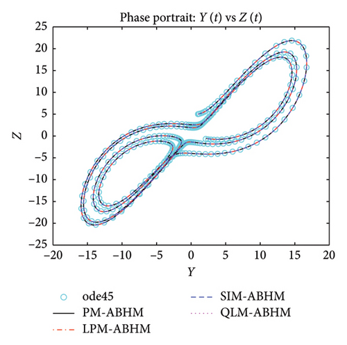
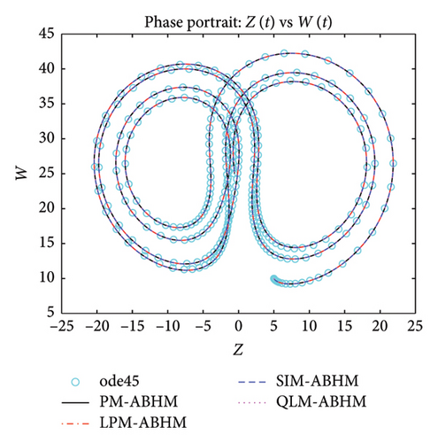
Figure 19 shows that the numerical solutions obtained by PM-ABHM, LPM-ABHM, SIM-ABHM, and QLM-ABHM demonstrate strong consistency with the reference solution computed using the ode45 MATLAB solver, as no exact solutions are available. This close agreement validates the effectiveness of the proposed methods in accurately solving Example 6.
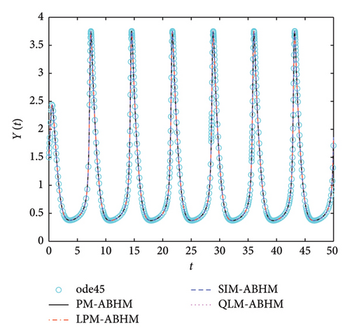
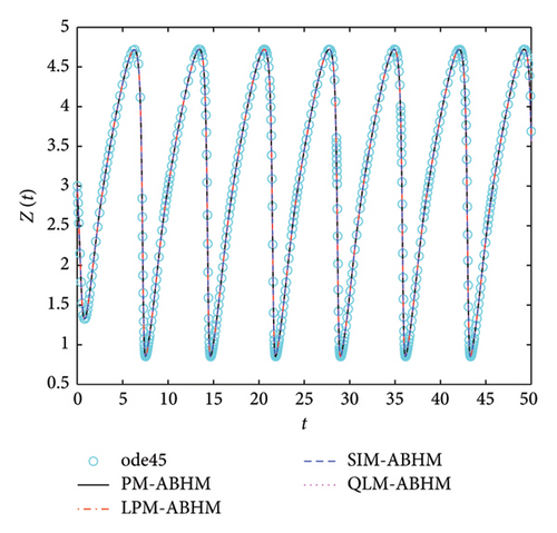
Table 8 gives a comparison of the maximum AE using the PM-ABHM, LPM-ABHM, SIM-ABHM, and QLM-ABHM at tF = 20 with various ABHMs [23, 71]. The results indicate that PM-ABHM, LPM-ABHM, SIM-ABHM, and QLM-ABHM consistently achieve the lowest errors across different h0 and Tol1, outperforming Opthbm and EMOHM. Additionally, PM-ABHM demonstrates the best computational efficiency in terms of CPU time.
| h0 | Tol1 | PM-ABHM | LPM-ABHM | SIM-ABHM | QLM-ABHM | EMOHM [71] | Opthbm [23] |
|---|---|---|---|---|---|---|---|
| 10−3 | 10−6 | 1.3412 × 10⁻¹¹ | 1.3421 × 10⁻¹¹ | 1.3413 × 10⁻¹¹ | 1.3408 × 10⁻¹¹ | 1.53089 × 10⁻⁹ | 1.2513 × 10⁻⁸ |
| CPU | 0.059026 | 0.300385 | 0.314092 | 0.325632 | — | 0.077 | |
| 10−4 | 10−7 | 1.7031 × 10⁻¹³ | 1.6931 × 10⁻¹³ | 1.7025 × 10⁻¹³ | 1.6875 × 10⁻¹³ | — | 9.6196 × 10⁻¹⁰ |
| CPU | 0.102599 | 0.450135 | 0.597188 | 0.515766 | — | 0.107 | |
| 10−1 | 10−10 | 5.8287 × 10⁻¹⁵ | 1.1324 × 10⁻¹⁴ | 1.2434 × 10⁻¹⁴ | 7.6050 × 10⁻¹⁵ | — | — |
| CPU | 0.698620 | 2.923950 | 3.880332 | 3.542907 | — | — | |
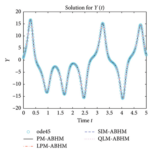
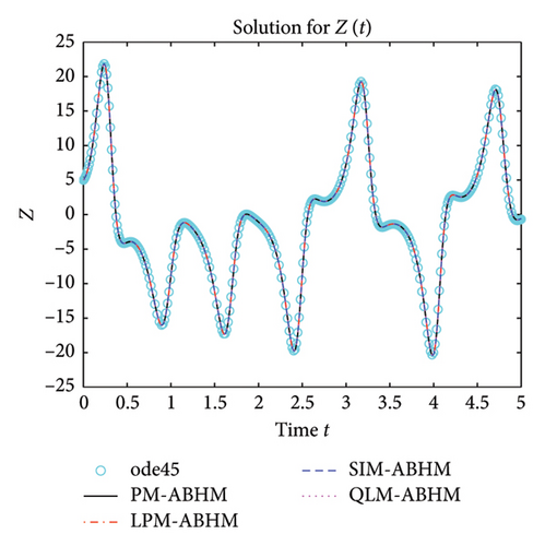
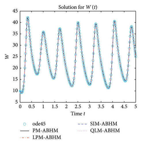
7. On the Application of the ABHM

8. Conclusion
- •
For the same initial step-size, all methods exhibit comparable effectiveness, indicating their suitability for high precision.
- •
By choosing the initial step-size and first user-defined tolerance small enough, we observed that the number of iterations per block required was reduced in all ABHMs.
- •
The PM-ABHM and QLM-ABHM consistently achieve the highest accuracy and efficiency, making them highly effective for applications demanding high precision.
- •
The QLM-ABHM, despite requiring the fewest iterations, achieves high accuracy and efficiency.
- •
The SIM-ABHM is slightly better than the LPM-ABHM in terms of accuracy and the number of iterations required per block.
- •
In terms of CPU time required, we noted that the PM-ABHM and QLM-ABHM are faster than SIM-ABHM and LPM-ABHM.
The insights gained from this work not only enhance the theoretical understanding of ABHM but also provide practical guidelines for selecting effective linearization methods. Future research could further implement the rational optimal grid points within ABHMs, combined with linearization techniques. Also, it could focus on implementing these methods to solve higher-order initial and BVPs, as well as enhancing their performance through more efficient tolerance settings. Additionally, developing new linearization techniques that surpass existing methods in terms of efficiency would represent a significant contribution.
Nomenclature
-
- EST
-
- Error estimation function
-
- Tol1
-
- First user-defined tolerance
-
- Tol2
-
- Second user-defined tolerance
Greek symbols
-
- σ
-
- Safety factor
Abbreviations
-
- AE
-
- Absolute error
-
- AEE
-
- Absolute error estimate
-
- ABHM
-
- Adaptive block hybrid method
-
- BHM
-
- Block hybrid method
-
- IVP
-
- Initial value problem
-
- PM
-
- Picard method
-
- SIM
-
- Simple iteration method
-
- LPM
-
- Linear partition method
-
- LTE
-
- Local truncation error
-
- QLM
-
- Quasi-linearization method
Conflicts of Interest
The authors declare no conflicts of interest.
Funding
No funding was received for this manuscript.
Acknowledgments
The authors are grateful to the University of KwaZulu-Natal and University of Zululand. The authors sincerely thank the editors and reviewers for their valuable and constructive feedback.
Open Research
Data Availability Statement
The data that support the findings of this study are available within the article.


