1. Introduction

The stratospheric airship is a common type of near-space, long-endurance aircraft that typically operates in the altitude range of 18–22 km in the lower stratosphere. In comparison to traditional aircraft and satellites, it possesses a distinctive combination of “time persistence” and “station keeping” capabilities, often referred to as the “stratospheric satellite” concept [1, 2].

Controlled flight is a crucial technology for stratospheric airships to maintain long-term station keeping. Effective trajectory tracking control is a significant aspect of controlled flight. Stratospheric airships, as controlled objects, possess characteristics such as large inertia, underdrive, strong perturbations in dynamic model parameters, and significant influence from environmental wind fields [3–6].

In the field of engineering, control strategies based on dynamic models often result in significant control errors related to state feedback and parameter identification [7, 8]. However, with the advancement of artificial intelligence technology, control methods that are independent of dynamic models have garnered considerable attention [9–11]. One such method is reinforcement learning (RL), which focuses on utilizing the interaction experience between agents and the environment. RL encompasses various algorithms such as Q-learning, state-action-reward-state ^′-action ^′ (SARSA), and Monte Carlo. By continuously interacting with the environment, RL generates action strategies without relying on supervised signals. This capability allows control systems to exhibit intelligent adaptive behavior in the face of model uncertainty and external disturbances. RL is extensively applied in controlling robots, autonomous underwater vehicles, drones, and other similar systems.

Leottau et al. [12] adopted the RL method to train and learn robot movements to achieve online control of posture and trajectory. Rastogi [13] adopted RL and applied deep deterministic strategy gradient method to online action learning of biped robots to achieve motion trajectory and attitude control. Ahmadzadeh et al. [14] proposed a RL method based on hierarchical structure to realize autonomous lifting and lowering of underwater vehicles by controlling valve action values. Khan [15] used the near-end strategy optimization algorithm to train the maneuvers of underwater vehicles and obtained the required return function value of the algorithm through multiple tests to achieve autonomous trajectory tracking. In literature [16], the RL method was introduced to establish MDP model of unmanned boat course tracking under complex sea conditions, and training samples were provided through experience pool playback technology. For multidimensional continuous state space tasks, Faust [17] adopted the learning model of first local and then generalization to realize autonomous flight control of four-rotor UAV.

The stability of stratospheric airships, along with their extended control time and nondestructive control actions, makes them suitable for the trial and error mechanism of RL. With a station keeping time of up to a month, there is ample opportunity for iterative estimation of action value functions. These characteristics create favorable conditions for implementing RL in the trajectory tracking control of stratospheric airships.

Reference [18] used a RL method to learn control parameters for indoor aerostat heading control, which improved the robustness of the controller, but the robustness of the controller is not verified. Rottmann et al. [19] designed the controller based on the Q-learning algorithm and carried out online training for the problem of aerostat cruise altitude control. However, the ε-greedy strategy is adopted to balance exploration and utilization, but it is a challenge to dynamically adjust the value of ε to achieve the optimal balance between exploration and utilization in different learning stages. In literature [20], the Q-learning algorithm was used to control low-altitude airships, and the discrete parameters of the state space were determined through two test movements to realize altitude and horizontal trajectory control, respectively. On this basis, three-dimensional trajectory tracking control was realized, which had large dynamic errors. For the horizontal trajectory tracking control problem, literature [21] changes the selection basis of the action strategy in the Q-learning algorithm and takes the relationship between the state and action obtained based on the dynamic model as training samples to reduce dynamic errors. Daskiran et al. [22] studied the tracking and control method of three-dimensional trajectory RL for low-speed airships. The main problem lies in the slow and complex learning process and the high time cost. Literature [21] proposes an adaptive horizontal trajectory control method for stratospheric airships in an uncertain wind field using the Q-learning algorithm, and a cerebellar model articulation controller (CMAC) neural network is designed to optimize the action strategy for each state. Literature [23] considered the thermal coupling characteristics of the airship; the trajectory tracking control of altitude direction is realized by using the deep RL method. However, neither of these two papers considered the problem of three-dimensional trajectory tracking control. The above studies are based on low-altitude airship or small indoor airship models. However, the operating environment of stratospheric airships is more complex and stratospheric airships are more easily affected by the environment, so the controller applied to stratospheric airships needs higher precision.

The chapter organization is as follows: Section 2 establishes the three-dimensional trajectory tracking control problem for stratospheric airship. Section 3 presents the design of the three-dimensional trajectory tracking controller for stratospheric airship. Section 4 provides the simulation analysis. Finally, the conclusion is presented in Section 5.

2. Three-Dimensional Trajectory Tracking Control Problem for Stratospheric Airship

The airship is an underdriven aircraft; it needs to rely on the horizontal symmetrical distribution of the propeller differential and then yaw. The dynamic model of horizontal direction can refer to the literature [25], and the dynamic model of altitude direction can refer to the literature [23].

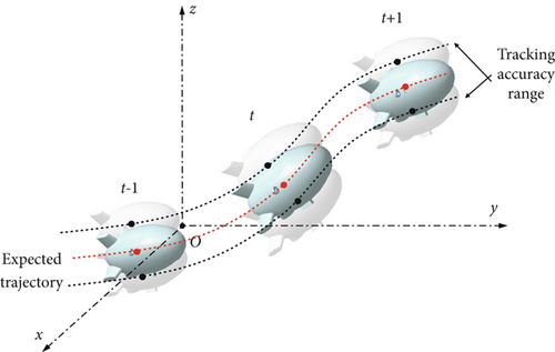
Actuators for tracking control of stratospheric airship three-dimensional trajectory may include motor speed (thrust vector magnitude), tilt angle of thrust vector device, elevator rudder deviation, rudder deviation, and fan-valve switch state. Stratospheric airship relies on floating weight to balance the standing space and has a large volume, resulting in a large additional mass and additional inertia. Due to the thin atmosphere in the stratosphere and the low efficiency of rudder surface control, control rudders are typically not installed on stratospheric airships. Instead, the tilt angle of the thrust vector device and the fan/valve state are coordinated to achieve the desired trajectory tracking control, and the airship’s wind resistance speed and wind speed are in the same order, and the trajectory control (position, speed, and yaw) is greatly affected by the wind field. The trajectory tracking control schematic of stratospheric airship is shown in Figure 1.

3. Design of Three-Dimensional Trajectory Tracking Controller for Stratospheric Airship

3.1. MDP Model

Based on the discrete state action space, the MDP model of the stratospheric airship trajectory tracking control problem is established [26].

3.1.1. State Space S

Stratospheric airship three-dimensional coordinates (x, y, z) are elements of the state space, and S = {s₁, s₂, ⋯s_i, ⋯, s_n}, state space of three-dimensional trajectory is shown in Figure 2.

3.1.2. Action Space A

State of tilt angle of thrust vector device and fan/valve combination were observed during horizontal trajectory control and altitude control. The coupling state of these two kinds of actuators is taken as the action value of controlling the three-dimensional trajectory. The action space can be expressed by A = {a₁, a₂, ⋯, a_i, ⋯, a_n}, a_i = (υ_i, τ_i).

The following simulation is divided into two types of action space, including the cube action-state space and the spherical action-state space. The action-state spaces are shown in Tables 1, 2, and 3, respectively.

Table 1. Relation between states and actions.

State	Action
Up	Inflation 2, zero thrust
Right, front, up	Inflation 1; push forward right
Right, back, up	Inflation 1; push forward left
Left, front, up	Inflation 1; push back right
Left, back, up	Inflation 1; push back left
Front	Closed; push forward right
Left	Closed; positive push back
Down	Deflate 2; zero thrust
Right, front, down	Deflate 1; push forward right
Right, back, down	Deflate 1; push forward left
Left, front, down	Deflate 1; push back right
Left, back, down	Deflate 1; push back left
Back	Closed; positive forward left
Right	Closed; positive push forward

Table 2. The relation between states and actions.

Tilt angle operation value of thrust device	Course angle increment
−π/3	−π/45
−π/4	-π/60
−π/6	-π/90
−π/12	-π/180
0	0
π/12	π/180
π/6	π/90
π/4	π/60
π/3	π/45

Table 3. The relation between states and actions.

Fan/valve operation value	Altitude increment
Inflation 6	−1
Inflation 5	−0.7
Inflation 4	−0.5
Inflation 3	−0.3
Inflation 2	−0.2
Inflation 1	−0.1
Closed	0
Deflation 1	0.1
Deflation 2	0.2
Deflation 3	0.3
Deflation 4	0.5
Deflation 5	0.7
Deflation 6	1

3.1.3. Reward R

The Euclidean distance between the position state after the state transfer and the expected reference state is used as a reward value or a penalty value:

$$ ()

where t indicates the current time and (x_c(t), y_c(t), z_c(t)) and R is the current state and reward of the moment. (x_{c(t + 1)}, y_{c(t + 1)}, z_{c(t + 1)}) is the state of the next moment. (x_r(t), y_r(t), z_r(t)) is the desired reference state for the current moment.

3.1.4. State Transition Probability P

Considering the characteristics of horizontal and vertical control comprehensively, the state transition probability and action selection are jointly determined by the flow direction angle and the size of the return value. Boltzmann random distribution based on the size of the return value and the deterministic distribution of the wind direction angle are adopted to jointly determine the action selection strategy. The state transition probability can be expressed as follows:

$$ ()

where $$ represents the value function estimate, T_temp is the exploration factor, and n_angle−i is the size of the wind angle.

3.1.5. Objective Optimization Function J

We set a certain simulation step length and accumulate discounts according to the time series for the return value obtained at each moment:

$$ ()

3.3. Three-Dimensional Trajectory Tracking Controller Flow

The three-dimensional trajectory tracking control flow for a stratospheric airship, based on the Q-learning algorithm and CMAC neural network, is illustrated in Figure 3. The specific control process is as follows:

• 1.

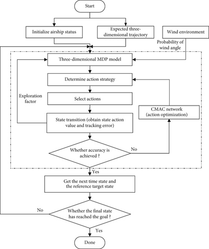
  Establish the expected reference three-dimensional trajectory for the stratospheric airship during its mission. Set the initial orientation and speed of the airship to obtain the initial state value and target state value. Define the position state as the state space, while the tilt angle state of the fan/valve and thrust vector device serves as the action space.

• 2.

  The wind angle probability of the future flow relative to the airship is considered the deterministic component of the action selection probability in the Q-learning algorithm. Simultaneously, the exploration factor, based on the Boltzmann distribution and derived from the estimated value of the action value function, constitutes the random component of the action selection probability. This step, combined with Step 1, allows for the construction of the MDP model for the stratospheric airship’s three-dimensional trajectory tracking control problem within a wind field.

• 3.

  Utilizing the known environmental wind field data, the CMAC network is trained. Each action input taken at each position state corresponds to a Q-value function. A CMAC neural network is established for each action value function, leading to the determination of the optimal value function and the corresponding action strategy, guided by the Boltzmann distribution.

• 4.

  According to the initial action strategy, the corresponding action is selected to obtain the state action value function and state tracking error after the state transition. The estimated value of the state action value function is taken as the component of the Boltzmann distribution, and the state tracking error is taken as the input of the CMAC network. The action strategy is updated, action selection is reperformed, and iteration is repeated. The tracking control error is used as the iteration termination criterion to obtain the optimal action.

• 5.

  According to the optimal action obtained, the state of the next moment and the reference target state are obtained, and whether the reference target state reaches the final target state is used as the criterion of whether the trajectory tracking control is over.

The advantages of CMAC compared to full connect neural networks are as follows:

• 1.

  CMAC is a neural network architecture based on local perception, making it particularly well-suited for processing sparse data in high-dimensional input spaces.

• 2.

  CMAC achieves local generalization by segmenting its input space into multiple small, overlapping receptive fields, which helps mitigate the influence of unrelated inputs on the output and enhances the model’s robustness.

• 3.

  Furthermore, CMAC’s approach to local generalization, through the division of its input space into multiple small, overlapping receptive fields, effectively reduces the impact of irrelevant inputs on the output, thereby improving the model’s overall robustness.

4. Results and Analysis

4.1. Simulation Condition

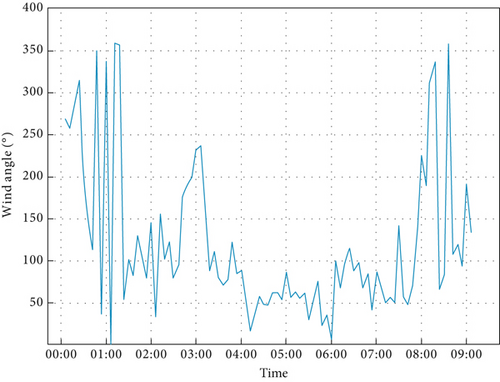
The simulation scenario is set as: the altitude of the stratospheric airship is adjusted from 18–18.5 km, the circling radius is set within the range of 500–1000 m, and the working area is Changsha. The wind direction distribution at zero every day near the altitude of 18 km in September is shown in Figure 4.

According to Section 2.1, the relation between the action value and the status change of the stratospheric airship is constructed; that is, the influence of the degree of fan/valve switch and the change of thrust vector transposition tilt angle on the position state of the airship.

In the initial training stage, according to the discrete action value range of horizontal heading control and altitude control, the corresponding action model range is set, the continuous action is discretized, and the action interval and the action range that can be executed under each state are set with reference to the actual flight conditions.

4.2. Tracking Results Under Cube Distribution

Regardless of the effective operation interval of the stratospheric airship, nine discrete state values are assigned to the tilt angle of the propulsion device and five action values to the fan/valve state. The relationship between action and state changes in the actual process is unknown, and specific actions are designed according to qualitative analysis to correspond to state changes, as shown in Table 1. In the table, Inflation 1 represents the number of fans opened as 1, Inflation 2 represents the number of fans opened as 2, Bleed 1 means the number of valves opened is 1, and Bleed 2 means the number of valves opened is 2.

Initially, each state has the same 14 transferable states and optional action values, as shown in Figure 5.

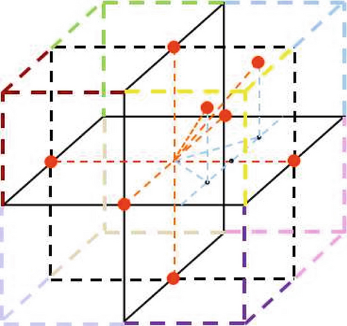
In the learning process of each iteration step, the optional action value in each state is selected and eliminated. After a certain period of learning, the action value corresponding to each state will be uniquely determined, and the action sequence corresponding to the whole process is the optimal action strategy. According to the above analysis, the input of CMAC neural network is 14 action values, and the output corresponds to 14 Q value functions. The tracking and control results of the stratospheric airship’s three-dimensional trajectory are shown in Figure 6, and the tracking and control errors are shown in Figure 7.

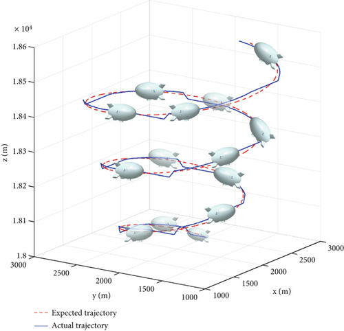
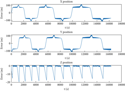
As can be seen from Figure 6, local mutations exist in the actual flight trajectory, and the transition smoothness needs to be improved. As can be seen from Figure 7, the maximum tracking control error in the horizontal direction is on the order of 100 m, while the tracking control error in the altitude direction is on the order of 10 m.

4.3. Tracking Results Under Spherical Distribution

Aiming at the large error of horizontal trajectory tracking control in the state transition cube distribution setting, the state change and action selection are optimized.

The airship is an underdriven aircraft; it needs to rely on the horizontal symmetrical distribution of the propeller differential and then yaw. The dynamic model of horizontal direction can refer to the literature [25], and the dynamic model of altitude direction can refer to the literature [23]. In the actual setting, the next state can be obtained by inputting corresponding actions according to the dynamic equation, and the mapping relationship between Table 2 and Tables 3 can be determined accordingly.

Considering the effective range of stratospheric airship operation, the variation range of the tilt angle of the propulsion device is limited to [−π/3, π/3], and tilt angle increment is set to π/12. There are nine discrete state values in total, and the relationship between the action values and the corresponding course angle increment is shown in Table 2. At the same time, the fan/valve state is refined into 13 states, and the relationship between the action value and the corresponding altitude increment is shown in Table 3.

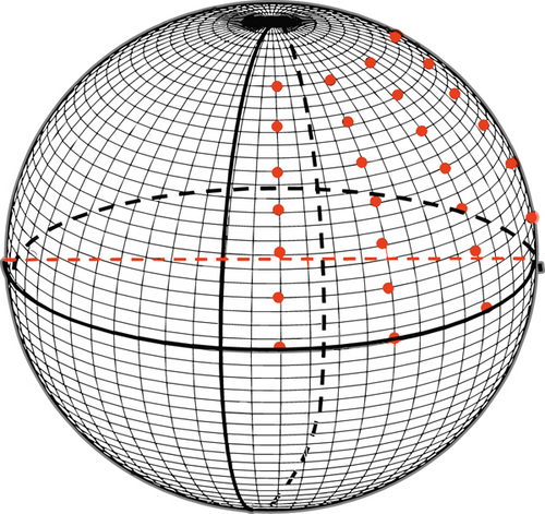
After the above adjustment, the state transition changes were transformed from 14 orientations of the cube distribution to 117 (9 × 13) of the spherical distribution, as shown in Figure 8. The state changes and action selection were more consistent with the actual motion situation. The motion value of the propulsion vector device is distributed on nine semiarcs of the sphere, and each semiarc is distributed with 13 state points (two vertices are shared by nine arcs).

The results of stratospheric airship’s three-dimensional trajectory tracking control are shown in Figure 9, and the trajectory tracking control error is shown in Figure 10.

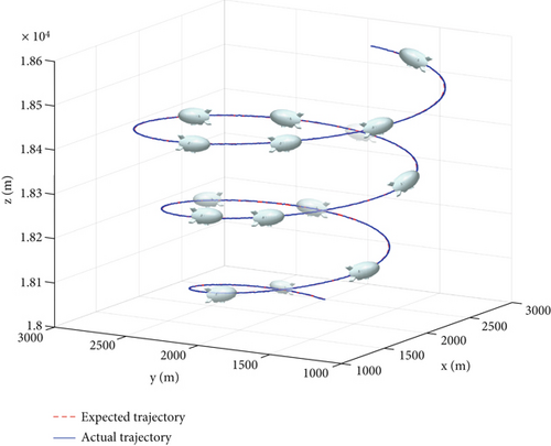
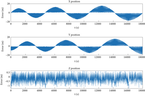
As can be seen from Figure 10, the actual flight trajectory of the stratospheric airship almost coincides with the expected reference trajectory, and the tracking control precision is high, the transition is smooth, and the project is well realized. As can be seen from Figure 11, the horizontal direction tracking control error is on the order of 10 m, and the altitude error is on the order of meters.

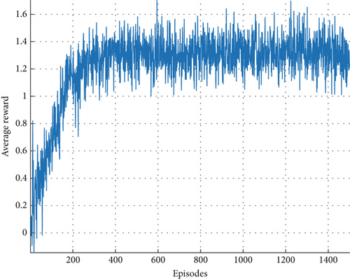
The average reward change curve of the training process is shown in Figure 11. It can be seen from the figure that the average reward obtained by the agent after 200 training episodes converges to a relatively gentle value, and the overall reward value shows an upward trend, and the effect is stable.

The simulation results show that the control accuracy of the three-dimensional trajectory tracking controller can be effectively improved by setting the effective action interval of the actuator reasonably and refining the distribution of the state action values.

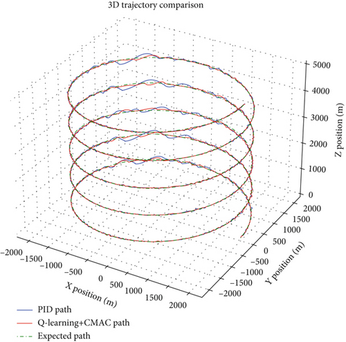
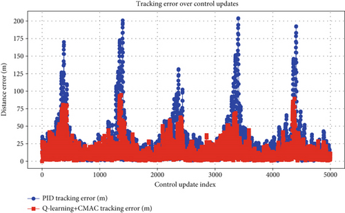
In order to verify the accuracy and robustness of the designed controller, factors of model parameter perturbation and ambient wind field disturbance are added and compared with the traditional PID controller. The results are as follows.

As can be seen from Figures 12 and 13, considering only the perturbation of model parameters, the average error of the PID controller is 12.67 m and the maximum error is 33.53 m. The average error of the controller in this paper is 6.69 m and the maximum error is 20.67 m, and the tracking accuracy is improved by 47.2% and 38.4%, respectively.

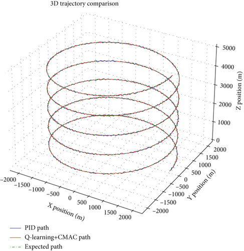
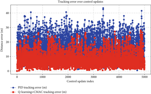
As can be seen from Figures 14 and 15, considering the perturbation of model parameters and the disturbance of ambient wind field, the average error of the PID controller is 24.18 m, and the maximum error is 203.96 m. In this paper, the average error of the controller is 14.05 m, the maximum error is 94.66 m, and the tracking accuracy is increased by 41.9% and 53.6%, respectively.

5. Conclusion

In future research on stratospheric airship trajectory control methods, it is important to consider the influence of thermodynamic characteristics on airship dynamics during modeling. Additionally, introducing a wind field uncertainty model could enhance the study of trajectory control effects.

Conflicts of Interest

The authors declare no conflicts of interest.

Author Contributions

Xixiang Yang: methodology, investigation, conceptualization, funding acquisition. Fangchao Bai: writing – review, visualization, supervision. Xiaowei Yang: writing – original draft and editing, Software. Yuelong Pan: editing, software, validation.

Funding

This work was supported by the Distinguished Young Scholar Foundation of Hunan Province, 10.13039/501100019338, 2023JJ10056 and the National Natural Science Foundation of China, 10.13039/501100001809, 52272445.