Advanced Solar Irradiance Forecasting Using Hybrid Ensemble Deep Learning and Multisite Data Analytics for Optimal Solar-Hydro Hybrid Power Plants
Abstract
Solar energy with hydropower power plants marks a significant leap forward in renewable energy innovation. The combination ensures a consistent power supply by merging the fluctuations of solar energy with the predictable storage provided by hydropower. This research aims to predict high solar irradiance on hydropower plants to maximize active power generation. A novel hybrid decomposed residual ensembling model for deep learning (SBLTSRARW) using models such as autoregressive integrated moving average (ARIMA) and seasonal-trend decomposition using loess (STL) along with prediction and optimization models such as Bidirectional LSTM (Bi-LSTM), and Whale Optimization Algorithm (WOA) methods are used to predict the irradiances. Various forecasting methods, including STL-Bi-LSTM, SBLTSAR, SBLTARS, and SBLTSRAR models, are assessed to determine their effectiveness in predicting solar radiation. The results show the accuracy of the proposed model, with RMSE and MAE values of 1.85 W/m2 and 1.31 W/m2, respectively. The proposed SBLTSRARW model results are more accurate than the Bi-LSTM, STL-Bi-LSTM, SBLTSAR, SBLTARS, and SBLTSRAR models, with RMSE value reductions of 517%, 217%, 151%, 98%, and 1%, respectively.
1. Introduction
Renewable energy is increasingly being used to offset the effects of climate change and global warming. The exploration of incorporating renewable energy sources into existing energy grids is gaining momentum [1]. Future energy supply will most likely rely heavily on solar and wind energy. Solar power is a rapidly developing renewable energy source and is unreliable and intermittent, affecting grid management [2]. Solar energy’s volatility and randomness also pose considerable integration challenges [3]. Adapting hybridization and forecasting ensures a reliable energy supply from intermittent sources.
The hybridization approach will integrate various renewable energy sources, such as combinations of hydro with floating solar, hydro with wind, hydro, solar, and wind together, to provide reliable renewable energy [4]. Hybridization-based research offers a sustainable solution to the world’s growing energy demands by combining the advantages of solar photovoltaic power plants with pumped storage power plants [5]. The efficiency of the combination is significantly enhanced by adapting floating photovoltaic (FPV) technology [6].
Installing floating PV panels on hydropower plants worldwide has the potential to generate over 4.4 GW of electricity with a surface coverage of just 2%, resulting in approximately 6270 TWh of electricity [7]. This type of hybridization is especially important for countries like India, where land for large-scale solar installations is limited [8]. Floating PV panels provide a cost-effective alternative that accelerates project timelines by avoiding complex land acquisition processes and preserving land for agricultural use. Additionally, covering reservoir areas with floating solar panels reduces water evaporation, increases water availability, and enhances hydropower generation. The cooling effect of the water further boosts the efficiency of PV panels installed on reservoirs [9].
The integration of floating PV panels with hydropower increases the flexibility of both energy sources, creating a “virtual battery” that supplies solar power during the day and relies on hydropower during periods of low solar radiation or at night [10]. Additionally, hydropower reservoirs for solar projects provide integrated grid connections and access to existing infrastructure, such as roads. Consequently, countries worldwide are implementing policies to encourage the adoption of hybrid solar systems based on hydropower, aiming to boost renewable energy production and reduce dependence on traditional hydropower alone [11].
Developing a highly dynamic power grid based on accurate solar forecasts offers a cost-effective hybrid technological solution to mitigate solar variability. The forecasting model integration presents significant advantages for power grid management and real-time power forecasting. It presents significant advantages for power grid management and real-time power forecasting [12]. It also aids energy managers in optimizing solar power generation, managing energy storage, and ensuring grid stability through accurate predictions. Surplus energy is stored or directed by high solar radiation period predictions, while backup power sources can be activated during low solar radiation periods. These predictive capabilities allow for real-time adjustments in energy flows, preventing grid overloads and ensuring efficient power distribution. As energy systems evolve, embedding this model within smart grids will enhance dynamic decision-making, improve overall grid stability, and support the integration of renewable energy sources, ultimately contributing to a more sustainable and reliable power supply. Therefore, these forecasts are essential for grid regulation, load-responsive production, power planning, and meeting feed-in obligations. As demand for solar energy integration rises, the need for diverse solar forecasting methods across various temporal and spatial resolutions grows, which enables cost-effective PV energy integration [13].
Accurately forecasting irradiance is complicated by clouds and dust, posing challenges for physical models. As a result, statistical methods such as autoregressive moving averages, support vector machines, and artificial neural networks are commonly used. However, these approaches struggle with problems such as low accuracy, and limited scalability with large data sets, and face difficulties in capturing long-term dependencies. Deep learning-based models, such as neural networks, particularly the multilayer perceptron, long short-term memory, and gate recurrent unit structure, are widely utilized to handle such complex nonlinear difficulties [14]. Fine-tuning the hyperparameters of these deep learning models can enhance prediction accuracy and is commonly achieved using optimization techniques such as genetic algorithms, whale optimization, and particle swarm optimization.
2. Literature Review
Solar irradiance was predicted using various forecasting models, from traditional methods to cutting-edge hybrid ensemble deep learning approaches [15]. Ghislain et al. [16] introduce a statistical spatiotemporal model to enhance the short-term forecasting accuracy of photovoltaic production. Addressing the nonstationarity issue of production series, they propose a stationarity process that significantly reduces forecasting errors compared to raw inputs. Their time series model, leveraging spatiotemporal dependencies among distributed power plants, offers low computational requirements and improves forecasting performance. Since solar irradiance data is nonstationary due to factors like clouds and seasons, traditional time series models struggle to capture nonlinearities, leading to poor prediction accuracy. Additionally, the large volumes of current data make these models less suitable. As a result, researchers have shifted their focus from traditional models to machine and deep learning approaches. Alzahrani et al. [17] introduced a solar irradiance prediction model employing deep recurrent neural networks LSTM, emphasizing preprocessing, supervised training, and postprocessing stages. The study utilized data from Canadian solar farms to demonstrate the effectiveness of LSTM, yielding a mean RMSE of 0.077 for the test dataset, outperforming other methods. Notably, LSTM’s enhanced data handling and feature extraction capabilities make it a promising tool for accurate solar irradiance prediction, overcoming deficiencies in traditional statistical methods like ARMA, and signaling its suitability for practical applications. Hosseini et al. [18] introduce a GRU-based approach for Direct Normal Irradiance forecasting, offering computational efficiency while maintaining accuracy comparable to LSTMs. They assess univariate and multivariate GRU, optimized using historical irradiance, weather, and cloud cover data from the LRSS solar facility in Colorado. Comparative analysis against LSTM models demonstrates the superiority of the proposed multivariate GRU, exhibiting a 34.42% improvement in RMSE and a 41.31% enhancement in MAPE. Additionally, the multivariate GRU showcases efficiency in forecasting multiple time horizons without compromising accuracy, highlighting its potential as a computationally effective solution for irradiance prediction. Liu et al. [19] research centered on utilizing Bi-directional Long Short-Term Memory (Bi-LSTM) neural networks. The study utilizes an 11-year weather dataset from NASA [20], employing preprocessing techniques such as Automatic Time Series Decomposition and Pearson correlation to enhance data quality by removing noisy values and selecting relevant features. A comparison analysis was carried out to compare Bi-LSTM’s performance to that of LSTM and MLP with Bi-LSTM being effective for solar irradiance forecasting. Individual models, however, have limits, driving researchers to explore hybrid models, which combine two or more models to maximize each’s capabilities. Babu et al. [21], and Reikard’s [22] forecasting experiment results highlight the dominance of ARIMA and hybrid model (ARIMA + ANN) across different resolutions and datasets. ARIMAs excel in capturing seasonal cycle transitions due to differencing at the 24-h horizon, while struggling with weather variability. Neural networks generally outperform regressions but lag behind ARIMAs, primarily due to training difficulties. The model choice depends heavily on resolution, with ARIMA better at lower resolutions dominated by seasonal cycles, and regressions or neural networks may excel at higher frequencies capturing short-term patterns. Hence, the combined approach (ARIMA + ANN) dominated both ARIMA and ANN when applied individually. Yinghao et al. [23] developed and applied a real-time re-forecasting ANN-GA optimization approach to predict intra-hour power generation from a 48 MWe PV plant. The re-forecasting approach notably improved forecast skills for time horizons of 5, 10, and 15 min across all baseline models, demonstrating its effectiveness in mitigating errors inherent in various forecasting methodologies. Huaizhi et al. [24] introduced a hybrid approach combining WT and DCNN for deterministic PV power forecasting for data from Belgian PV farms. WT decomposes the signal into frequency series, enhancing its outlines and behaviors, while DCNN extracts nonlinear features from each frequency. Additionally, they propose a probabilistic PV power forecasting model integrating deterministic methods with spine quantile regression to assess probabilistic information in PV power data. Application of these methods to PV data from Belgian PV farms shows improved forecasting accuracy across seasons and prediction horizons compared to traditional models. The model makes it suitable for processing real-time data in power plant operations. Cunha et al. [25] focus on improving the accuracy of the hybrid forecasting model by combining STL with SES and ARMA models. STL handles high-frequency time series data, while SES and ARMA models fit the trend and remainder components respectively. Applied to wind speed forecasts, the hybrid model achieved a significant 101.39% decrease in MAPE compared to ECS forecasts. Using Dense, LSTM, Conv1D, and STL. Njogho et al. [26] evaluate seven ensemble models with hydro data from the Lom Pangar reservoir. The results underline the superiority of the multivariate STL-dense model and highlight the importance of incorporating multiple inputs and models for improved prediction accuracy. Jun et al. [27] address the issue of a large and dynamic dataset of air pollution management through accurate prediction of pollutant concentrations. The proposed ARIMA-Whale Optimization Algorithm (WOA)-LSTM model combines ARIMA for linear data extraction and WOA-LSTM for nonlinear prediction, where the LSTM hyperparameters are optimized using the Whale algorithm. A comparative analysis with other models shows the superior performance of ARIMA-WOA-LSTM in pollutant prediction accuracy, overall model accuracy, and prediction stability. Moreover, the combined model outperforms the individual models in these aspects, underlining the effectiveness of the proposed approach for air pollution management. Hang et al. [28] introduce a novel method for predicting aviation failure events by integrating seasonal-trend decomposition using Loess (STL) with a hybrid model comprising a transformer and autoregressive integrated moving average (ARIMA). STL decomposition isolates trend, seasonal, and remainder components, enhancing understanding of event characteristics. The transformer handles trend prediction, addressing computational efficiency issues, while ARIMA manages seasonal and remainder components, reducing complexity without sacrificing accuracy. Evaluation using ASRS data shows that the STL-Transformer-ARIMA model outperforms single models, demonstrating superior accuracy and robustness in predicting aviation failure events.
This literature sets the hybrid ensemble deep learning models, which integrate the strengths of diverse forecasting techniques to enhance prediction accuracy and robustness. Specifically, the STL model captures the trend, seasonal, and residual components with high interpretability. Statistics-based predictors are easy to use and allow for the quantification of each component’s effect. While they perform well with independent samples, these approaches often introduce significant uncertainty when dealing with complex, nonlinear relationships. Deep learning predictors excel at modeling such complex nonlinearities by learning from data samples and self-optimizing based on newly labeled data, which improves the understanding of solar irradiance trends and enhances forecast confidence. Additionally, a Bi-LSTM-based deep learning model is used to forecast the trend component, while the residual components are predicted using a novel multihead attention mechanism and parallel processing, which significantly improves accuracy for long sequence datasets. Hence, this research follows the remainder and residual decomposition using STL using Loess and ARIMA, prediction using Bi-LSTM, optimization using a WOA, and recomposition for combining the entire results to improve the solar radiance estimations.
- 1.
To develop a highly accurate hybrid ensemble intelligent deep learning forecasting model through the decomposed residual ensemble technique.
- 2.
To predict the high solar irradiance on hydropower houses to achieve high active power by reducing the error.
- 3.
To design the feasible hybrid model that supports the installation of hybrid hydro solar powerhouses to enhance reliability in hybrid green power generation with FPV advantages.
3. Theories and Methods
The individual models incorporated into the proposed hybrid ensemble model are detailed below: (i) STL, (ii) ARIMA, (iii) Bi-LSTM, and (iv) whale optimization.
3.1. STL
This method partitions the time series into three components: the remainder term, representing irregular variations; the trend term, capturing low-frequency patterns; and the seasonal term, reflecting high-frequency variations.
3.2. ARIMA Model
The Augmented Dickey-Fuller (ADF) test validates the data, which produced q, s, and d values. The AR (q) and MA (s) values were determined using the partial autocorrelation function (PACF) and the ACF functions. The ‘d’ value is determined by differencing the data [31].
3.3. Bi-LSTM Model
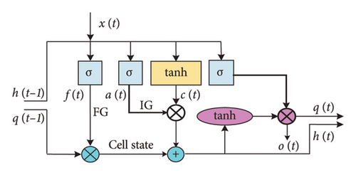
The Bi-LSTM network comprises multiple LSTM cells operating bi-directionally as in Equations (3)–(9). The forward layer processes information from the previous and current blocks, while the backward layer, with a reverse direction, utilizes information from future blocks.
3.4. WOA
-
Step 1: Mathematical Modelling
()() -
In this equation, “t” represents the current iteration, while “J” and “K” denote coefficient vectors. “Sp” signifies the position vector of the prey, and “S” indicates the position of a grey wolf. If an improved solution arises after iterations, S∗ updates. Then, the vectors J and Z are computed utilizing the equations
()() -
The range of fluctuation for variable Z is also reduced by z. In essence, Z is a random number within the interval [−z, z], where the value of z decreases from 2 to 0 over successive iterations.
-
Step 2: Exploitation Phase
-
Two strategies to mathematically emulate the humpback whale’s behavior in bubble nets:
- 1.
Shrinking mechanism
-
The mathematical representation of the behavior of grey wolves surrounding prey during the hunt is as follows:
()() - 2.
Spiral updating position
-
Initially, the process involves calculating the distance between the whale at position (S, T) and the prey at position (S∗, T∗). Subsequently, a spiral equation is formulated between the whale’s position and that of its prey to replicate the helix-shaped movement observed in humpback whales [34].
() -
In the equation, K′ denotes the distance between the i-th whale and the prey, where c is a constant determining the logarithmic spiral shape, and the variable n represents a random number selected from the range of [−1, 1].
() -
The humpback whales exhibit simultaneous movement patterns, swimming in both a diminishing circle and spiral around their prey. Apart from the bubble-net technique, humpback whales also engage in random prey searching. The mathematical representation of this search process is as follows.
-
Step 3: Search for prey
-
Exploration of prey can be a similar method by adjusting the A vector. Humpback whales naturally engage in random search behaviors depending on their respective locations. ‘A’ value higher than one or lower than minus one is employed to encourage search agents to move away from a designated reference whale. During the exploration phase, the position of a search agent is updated based on a randomly chosen search agent, rather than the best one discovered thus far during the exploitation phase [35]. By employing this method alongside |A| > 1, which promotes exploration, the WOA algorithm effectively conducts global searches. The mathematical representation is as follows:
()() -
where Srand represents a randomly selected position vector, corresponding to a random whale chosen from the current population. The conditions that activate the method to search are as follows:
() -
The global search capability of WOA and the susceptibility to local optimizations are due to the random nature of the variable “p” and the fact that a global search only occurs when “p” is less than 0.5.
4. Proposed Hybrid Ensemble Forecasting Methodology
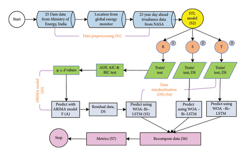
The proposed hybrid ensemble approach is explained in detail through a step-by-step process, illustrated in Figure 2, with the workflow depicted in Figure 3(b). The workflow, outlined through subsections, meticulously elaborates each step denoted as S1, S2, … S7 in Figure 3(b), offering a comprehensive understanding of the process.

4.1. Data Collection and Preprocessing
4.1.1. Data Collection
From the Ministry of Energy, India, the probabilistic analysis is performed for 252 high-scale hydropower locations by using 40 years day ahead solar irradiance data from NASA power database with latitude and longitude of selected locations taken from global energy monitor and twenty-five hydropower houses are selected [36].
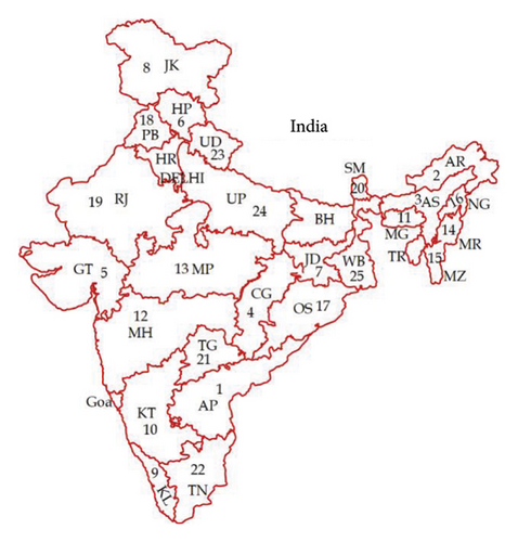
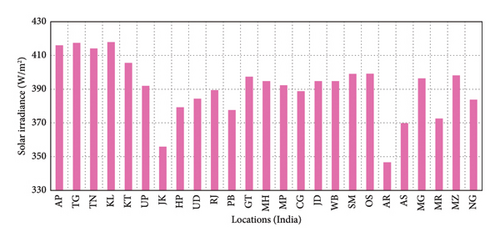
The results of the probabilistic analysis identify the following twenty-five hydropower plants as the most suitable locations for implementing optimal PV-hydro hybrid systems: Nagarjuna Sagar (AP), Pulichinthala (TG), Kodaya (TN), Idukki (KL), Kalinadi (KT), Rihand (UP), Sewa (JK), Tangnu Romai (HP), Khatima (UD), Jawahar Sagar (RJ), Mukerian (PB), Ukai (GT), Tillari (MH), Omkareshwar (MP), Hasdeo Bango (CG), Panchet (JD), Maithon (WB), Teesta (SM), Chiplima (OS), Ranganadi (AR), Kopili (AS), New Umtru (MG), Loktak (MR), Tuirial (MZ), and Doyang (NG) The identified Hydropower plant locations are shown in Figure 3(a). The average solar irradiance at these hydropower locations is shown in Figure 4.
4.1.2. Data Preprocessing
The single dataset contains only 14,560 samples with sixteen features on each location, hybrid deep learning models like LSTM, GRU and their ensembles are insufficient to handle the dataset. Therefore, twenty-five datasets [37] are mixed to form a large dataset of 364,000 samples divided into 80% train and 20% test datasets. Minor gaps were rectified using mean or median imputation and forward/backward filling. Particular rows or columns with significant missingness were eliminated to maintain data integrity. This comprehensive dataset encompasses twenty-five locations and includes only highly correlated features such as the clearness index, wet bulb temperature, surface pressure, solar irradiance, earth skin temperature, specific humidity, relative humidity, corrected precipitation, temperature, dew point, wind speed, and wind direction at 2 m/s and 10 m/s, among others.
The correlation analysis performed on solar irradiance indicates multiple significant correlations between the characteristics as in Figure 5. The strongest correlation is seen with wet-bulb temperature (0.87), followed by specific humidity at 2 m (0.68), showing that these parameters have a significant positive impact. Air temperature has a moderate correlation of 0.59, while dew point also correlates with 0.67, indicating that temperature, humidity, and dew point variables are important in forecasting solar irradiance. Other characteristics with a positive, but less obvious, include surface temperature at 0.52 and wind speed at 2 m at 0.43. Wind speed at 10 m shows a lesser but positive of 0.40, followed by precipitation and relative humidity at 2 m, with correlations of 0.20 and 0.07, respectively.
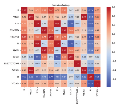
Additionally, we have added the latitude and longitude columns into the merged dataset to predict solar irradiance in particular locations. Another reason for merging the datasets is that using the model individually on each dataset will increase the computational time. Also, the model produces different errors for various locations, which leads to inaccuracies in forecasting solar irradiance for each location.
4.2. Data Decomposition Using STL
4.3. Remainder Data Decomposition or Data Double Decomposition
4.4. Data Standardization
4.5. Predictions Using Bi-LSTM Model
Bidirectional LSTM, distinguished by its ability to consider both past and future contextual information in data analysis, operates by processing input data in ascending order for future prediction and decreasing order for past context evaluation. The residuals from the ARIMA model, trend, and seasonal data from the STL model are passed individually into the Bi-LSTM model. This model runs the individual data through the LSTM cells bidirectionally and predicts the trend, seasonal, and remainder, respectively. Optimizing hyperparameters is pivotal in maximizing the performance of deep learning models, necessitating the fine-tuning of parameters such as batch size (BS), learning rate (LR), neuron (NN) count, and epochs for optimal results. Initially, the Adam optimizer including default settings with a LR of 0.01, 100 NN, a BS of 64, and 100 epochs was employed for the Bi-LSTM model. Subsequently, these parameters were refined using a whale optimization algorithm. Monitoring training and testing errors across epochs revealed a notable decrease in training loss within the initial 25 epochs, followed by a slower decline until convergence around the 70th epoch. Similarly, the test loss exhibited a comparable pattern, reaching convergence around the 60th epoch. Based on these findings, the study determined that the model attains high accuracy when trained for 100 epochs. This iterative process was repeated for various training/test splits and epoch configurations. The same approach was applied to tune hyperparameters for Bi-LSTM models handling trend, seasonal, and decomposed remainder data. The decision to employ this model solely for grouping 25 datasets rather than applying it to each dataset is due to computational time and efficiency concerns. Utilizing the model for individual datasets would entail 72 Bi-LSTM optimizations and 24 ARIMA parameter adjustments across the 25 datasets in addition. Therefore, consolidating the datasets simplifies the optimization process and large data increases the efficiency considerably.
4.6. Re-Composition of Predictions
The trend, seasonal, and remainder predictions from the three WOA—Bi-LSTM models are ensembled to obtain final prediction results. These predictions are further compared with various graphs and tables in the results and discussion section.
5. Metrics
Metrics play a crucial role in evaluating the performance and accuracy of solar radiation prediction models. These metrics provide quantitative measures that help to test the reliability and effectiveness of predictions to support decision-making processes in various applications related to solar energy [39]. Some of the key metrics used in solar irradiance prediction are as follows.
5.1. Mean Absolute Error (MAE)
MAE is suitable for regression problems and overall forecast evaluation, with smaller values indicating better forecasting performance.
5.2. Root Mean Square Error (RMSE)
6. Results and Discussions
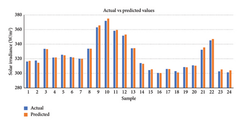
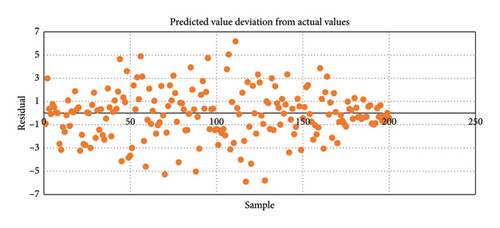
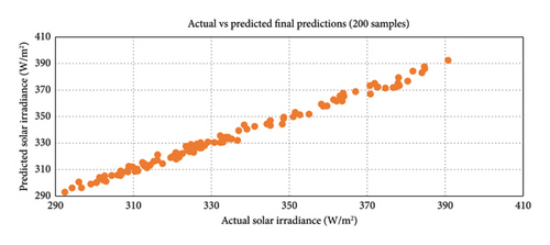
The predictions of trend, seasonal, and residual components derived from the proposed model, highlighting the comparison between actual and predicted values of the STL decomposed components, are presented in Figures 6, 7, 8. The recomposed predictions from the proposed model, featuring scatter plots depicting actual versus predicted values, along with various error plots derived from these recomposed predictions, are shown in Figures 9, 10, 11. The experimental results were obtained using Jupyter Notebook and Google Colab, with the necessary Python libraries installations. We employed a graphical processing unit (GPU) facilitated by the CUDA and CUDNN installation software tools to expedite processing, especially given the extensive use of epochs. This GPU integration significantly accelerated computations compared to standard CPU processing. Notably, Google Colab, with its GPU capabilities, was also leveraged for comparative analyses involving deep learning models.
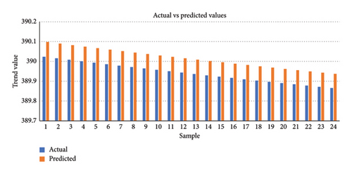
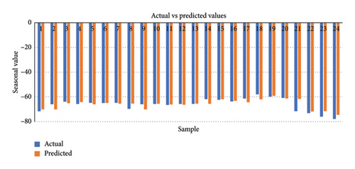
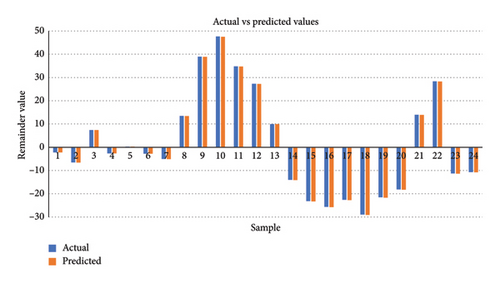
LSTM-based models displayed superior accuracy than Transformer models in several circumstances, indicating their efficacy in certain settings [40]. The results of the transformer and Bi-LSTM model are close to each other in our case. Bi-LSTM provided better results than the transformer model, especially in mean absolute error for a single layer. Therefore, this research uses the Bi-LSTM model as a benchmark. The third approach, STL-Bi-LSTM, involves decomposing the data using the Loess model’s residual, seasonal, and trend decomposition. The resulting trend, seasonal, and residual components are then individually fed into three Bi-LSTM models. Subsequently, the predictions from these models are combined to produce the ensembled result. The SBLTSAR model involves passing only the decomposed residuals into an ARIMA model, and the other trend and seasonal components are fed directly into Bi-LSTM models after STL decomposition. The results from these three models are combined to obtain the ensembled result. In the SBLTARS model, the residuals and seasonal components undergo ARIMA predictions, while the trend component is through a Bi-LSTM model. The results from these three models are combined to obtain the ensembled result. In the SBLTSRAR model, the decomposed residuals are passed through an ARIMA-Bi-LSTM model, while the seasonal and trend components are into Bi-LSTM models. The predictions from these models are then combined to predict the ensembled result. Furthermore, the Bi–LSTM model included in the SBLTSRAR approach is whale-optimized to achieve final optimal results. It is important to note that the ARIMA model is not for trend data due to the nonstationary nature of trend data, which renders the ADF test ineffective. Therefore, models utilizing ARIMA for trend data may not yield accurate results. The comparison of these different models is in Table 1. The results demonstrate the accuracy of the proposed decomposed residual ensembling bidirectional long short-term memory SBLTSRARW model with low RMSE and MAE values.
| Model | RMSE (W/m2) | MAE (W/m2) | Conclusion |
|---|---|---|---|
| Transformer | 11.85 | 8.65 | BS = 64, NN = 100, Epochs = 100, LR = 0.01 |
| Bi—LSTM | 11.42 | 8.20 | BS = 64, NN = 100, Epochs = 100, LR = 0.01 (reference model) |
| SBLTSAR | 5.87 | 4.08 | BS = 64, NN = 100, Epochs = 100, LR = 0.01 for Bi-LSTM (T and S), ARIMA (2, 0, 2) for R components |
| STL—Bi—LSTM | 4.65 | 3.17 | BS = 64, NN = 100, Epochs = 100, LR = 0.01 (T, R, and S) |
| SBLTARS | 3.67 | 2.46 | BS = 64, NN = 100, Epochs = 100, LR = 0.01 for Bi-LSTM (T), ARIMA (2, 0, 2) for R, S components |
| SBLTSRAR | 1.87 | 1.32 | BS = 64, NN = 100, Epochs = 100, LR = 0.01 for Bi-LSTM (T, S, and R), ARIMA (2, 0, 2) for R, S components |
| SBLTSRARW | 1.85 | 1.31 | BS = 64, NN = 67, 90 and 66, Epochs = 100, LR = 0.08, 0.09, and 0.003 for Bi-LSTM (T, S, and R), ARIMA (2, 0, 2) for R components |
7. Conclusion
This study investigates various forecasting approaches for solar irradiance prediction, ranging from bidirectional LSTM models to more advanced hybrid techniques, by predicting optimal locations of hydropower houses in India for high solar irradiance to generate the maximum power using the proposed model SBLTSRARW to confirm the reliable power supply. It also highlights the usefulness of applying intelligent time-series forecasting approaches, such as ARIMA, to include deep learning in renewable energy forecasting. By incorporating both trend, seasonal, and residual fluctuations, the model gives a thorough knowledge of solar energy trends in HSHP locations. Further, the outcome of this study is based on the proposed model SBLTSRARW, which identified the optimal locations (KL, AP, and TN) to generate the maximum power. Combining the datasets improved the consistency of error differences across all locations, enhancing the overall accuracy. The proposed SBLTSRARW model root mean square error values are lower than Bi-LSTM, STL-Bi-LSTM, SBLTSAR, SBLTARS, and SBLTSRAR models, with reductions of 517%, 217%, 151%, 98%, and 1%, respectively. The RMSE and MAE errors of SBLTSRAR and SBLTSRARW are closer to each other with 1.87, 1.32, and 1.85, 1.31 W/m2, respectively, as shown. It shows a slight improvement through the whale optimization model. This study also reduces computation time and increases the model performance by consolidating a single significant dataset analysis with twenty-five location data rather than processing each dataset individually. The achieved results validate the effectiveness of the proposed decomposed residual ensembling Bi-LSTM (SBLTSRARW) model, paving the way for further advancements in forecasting renewable energy systems. This work helps to initiate the installation of hybrid hydropower plants that improve the reliability of energy supply from generation to consumer, with the benefit of FPV systems. Furthermore, the precise and reliable GHI predictions created by the proposed method assist microgrid management, allowing operators to optimize energy storage, cut costs, and increase dependence on hybrid hydrosolar power. The model’s projections enable real-time changes in energy flows to avoid grid overloads and maintain efficient power distribution. As energy systems improve, integrating this model into smart grids will allow dynamic decision-making, increase overall grid stability, and facilitate the integration of renewable energy sources for a stable power supply. It also aids in attaining the Sustainable Development Goals.
7.1. Future Recommendations
Future research should focus on real-time adaptive forecasting systems that dynamically change in response to incoming data. This technology would enable more responsive energy storage management and ensure efficiency by better matching renewable energy characteristics and equitable cost allocation. In addition, model development tailored to specific climate zones such as tropical, temperate, and arid regions could increase the model’s accuracy and applicability across diverse environments.
Nomenclature
-
- SI
-
- Solar irradiance
-
- T2MWET
-
- Wet-bulb temperature
-
- T2M
-
- Air temperature
-
- T2MDEW
-
- Dew point temperature
-
- TS
-
- Surface temperature
-
- QV2M
-
- Specific humidity
-
- PS
-
- Surface pressure
-
- RH2M
-
- Relative humidity at 2 meters
-
- PRECTOTCORR
-
- Precipitation
-
- WS10M
-
- Wind speeds at 10 meters
-
- WS2M
-
- Wind speeds at 2 meters
-
- WD10M
-
- Wind direction at 10 meters
-
- ADF
-
- Augmented Dickey-Fuller
-
- AIC
-
- Akaike information criteria
-
- BIC
-
- Bayesian information criteria
-
- ARIMA
-
- Autoregressive integrated moving average
-
- T
-
- Trend
-
- S
-
- Seasonal
-
- R
-
- Remainder
-
- STL
-
- Seasonal-trend decomposition using loess
-
- Bi-LSTM
-
- Bidirectional LSTM
-
- WOA
-
- Whale optimization algorithm
-
- RMSE
-
- Root mean square error
-
- nRMSE
-
- Normalized root mean square error
-
- MAE
-
- Mean absolute error
-
- MAPE
-
- Mean absolute percentage error
-
- PV
-
- Photovoltaic
-
- FPV
-
- Floating photovoltaic
-
- PACF
-
- Partial autocorrelation function
-
- ACF
-
- Autocorrelation function
-
- AR
-
- Autoregressive
-
- I
-
- Integrated
-
- MA
-
- Moving average
-
- ANN
-
- Artificial neural network
-
- LSTM
-
- Long short term memory
-
- GRU
-
- Gate recurrent unit
-
- RNN
-
- Recurrent neural network
-
- GA
-
- Genetic algorithm
-
- PSO
-
- Particle swarm optimization
-
- DNI
-
- Direct normal irradiance
-
- ATSD
-
- Automatic time series decomposition
-
- KNN
-
- K—nearest neighbour
-
- WT
-
- Wavelet transform
-
- DCNN
-
- Deep convolutional neural network
-
- QR
-
- Quantile regression
-
- ECS
-
- Environmental control system
-
- SES
-
- Simple exponential smoothing
-
- LR
-
- Learning rate
-
- NN
-
- Neuron number
-
- BS
-
- Batch size
-
- GPU
-
- Graphical processing unit
Conflicts of Interest
The authors declare no conflicts of interest.
Author Contributions
All authors contributed to the study, conception, and model design. All authors commented on the manuscript. All authors read and approved the final manuscript.
Funding
No funding was received for this manuscript.
Open Research
Data Availability Statement
Data that were used to obtain the results are available from the corresponding author upon request.


