International Transactions on Electrical Energy Systems

Volume 2025, Issue 1 3620842

Research Article

Open Access

Optimal Transmission Switching for Congestion Management and Cost Reduction Using Linearized AC Optimal Power Flow

Mohammad Habibi,

Mohammad Habibi

orcid.org/0009-0007-3544-9106

Electrical Engineering Department , Shahid Rajaee Teacher Training University , Tehran , Iran , srttu.edu

Search for more papers by this author

Ali Zangeneh,

Corresponding Author

Ali Zangeneh

[email protected]

orcid.org/0000-0001-9899-5912

Electrical Engineering Department , Shahid Rajaee Teacher Training University , Tehran , Iran , srttu.edu

Electrical and Computer Engineering Department , Kharazmi University , Tehran , Iran , khu.ac.ir

Search for more papers by this author

Mohammad Habibi,

Mohammad Habibi

orcid.org/0009-0007-3544-9106

Electrical Engineering Department , Shahid Rajaee Teacher Training University , Tehran , Iran , srttu.edu

Search for more papers by this author

Ali Zangeneh,

Corresponding Author

Ali Zangeneh

[email protected]

orcid.org/0000-0001-9899-5912

Electrical Engineering Department , Shahid Rajaee Teacher Training University , Tehran , Iran , srttu.edu

Electrical and Computer Engineering Department , Kharazmi University , Tehran , Iran , khu.ac.ir

Search for more papers by this author

First published: 25 February 2025

https://doi.org/10.1155/etep/3620842

Academic Editor: Johny Renoald A.

Share a link

Email
Wechat
Bluesky

Abstract

Several approaches have been introduced to manage congestion in transmission lines while simultaneously reducing the generation cost of power systems. Two of these approaches, namely, generation rescheduling and transmission switching are used together in this article. Changing the system topology through optimal transmission switching (OTS) is an important and active research area in power systems for this purpose. Essentially, OTS is a mixed-integer nonlinear programming (MINLP) problem that is inherently nonlinear and nonconvex. Therefore, solving this nonlinear problem poses significant challenges for researchers. On one hand, there is no guarantee of reaching a global optimal solution, and on the other hand, issues such as the lack of convergence and increased solution time have made it difficult to solve the OTS problem. Linearizing the OTS problem provides a guaranteed method for reaching a comprehensive optimal solution. This study presents a new linear mathematical model for the OTS problem. The proposed model is solved using mixed-integer linear programming (MILP), which accurately determines the opening or closing status of transmission lines and the number of lines that should be opened to reduce the generation and congestion costs in the network. To this aim, a linear programming and piecewise approximation, along with Taylor’s series approximation method, is used to linearize the generation cost function, and AC optimal power flow equations. To reduce the solution time of the OTS problem without losing accuracy, a congestion cost index is used based on decreasing the total congestion cost of transmission lines, as well as the production cost of generators. The proposed model is implemented on IEEE 9-bus and IEEE 118-bus standard test systems. Also, in order to analyze the reliability of the system before and after switching, two methods of contingency analysis and calculation of the LOLP index have been used. The obtained results show that transmission switching can reduce the generation cost and the total power system congestion cost as well.

1. Introduction

There are various methods to control and improve the state of power systems operation. One of the key and useful ways to increase the power system’s efficiency from a number of angles is to rearrange the network’s topology and organization by switching the transmission lines. Previous studies have investigated transmission line switching as a control method to improve the voltage profile, manage congestion, increase the transmission capacity and flexibility, reduce generation cost, and increase the reliability and efficiency of the transmission network [1, 2]. Reference [3] provides a wide review of the optimal transmission switching (OTS) problem with respect to numerous operational concerns, as well as an analysis of the connection between OTS and other flexibility choices in power systems. A new asynchronous parallel heuristics method to generate good candidate solutions to speed up conventional branch-and-bound algorithms is proposed in [4]. In [5], using the decomposition and coordination method based on the alternating direction method of multipliers (ADMMs), an economic distribution model for interconnected system considering OTS is proposed. The effect of OTS in terms of power flow and voltage angles of the buses using DC optimal power flow (DCOPF) was studied in [6]. In [7], a heuristic switching method based on neural networks is presented to solve the OTS problem, in which it provides almost instantaneous switching actions using DCOPF equations. The decomposition approach is employed to model and investigate the impact of transmission switching (TS) on integrated generation and transmission maintenance scheduling. In order to guarantee system security, N-1 contingency constraints are taken into account [8]. Reference [9] develops an optimized network expansion planning model considering OTS to design an optimal investment plan for the construction of new transmission lines and generation units using the DCOPF method. In [10], OTS problem is considered to identify power system topology, assuming that certain lines are fixed (uncontrollable) and the others are controllable via on/off switches. The goal is to minimize the generation cost of the system and meet the physical and operational constraints at the same time. A multiobjective optimization approach based on DCOPF is proposed in [11] to optimize multiobjective functions simultaneously and address multiple solutions to line switching. Boshi et al. [12] suggest using OTS to eliminate voltage violations. Their suggested model is solved by a decomposition method as a mixed integer nonlinear program (MINLP) using AC optimal power flow (ACOPF) and binary variables. A two-level iterative framework with a mixed-integer quadratic cone programming OTS model providing candidate solutions at the top level and an AC feasibility assessment conducted at a lower level is used in [13] to present a novel OTS model that takes AC feasibility into account. The optimal switching of transmission lines for unit commitment with consideration of system security constraints was analyzed in [14–16]. In [17], a novel three-stage stochastic and robust OTS model is used to solve the OTS problem with N-k security constraint for power systems with high renewable energy penetration. In order to address the multiperiod optimization of the total operating cost using the DCOPF model, the combined OTS model and thermal unit commitment are presented in [18]. The OTS model with DCOPF is used in [19] to reduce system operating costs considering renewable energy sources and decomposing the power system into several subsystems using the analytical target cascading method. A method using a sequentially restricted quadratic program is developed and assessed in order to effectively address a coupled issue of OTS and optimal power flow, as described in [20]. Its nonlinear equality constraints, as well as the objective function, and inequality constraints are approximated in a quadratic form. In [21], using a hot start solution based on the CPLEX algorithm, the OTS problem is incorporated in solving the unit commitment considering the high penetration of wind power generation.

Changing topology of the power system can be used as a tool to manage congestion in the electrical network. This issue was studied and analyzed by various methods, such as genetic algorithms, as well as single-level and multilevel mathematical models [22, 23]. In [24, 25], OTS is applied via DCOPF to release the overload of transmission lines. The objective function of problem is defined as minimizing the number of transmission lines to be opened to release the overload. In [26], reducing of line power density through the use of OTS was investigated. The DCOPF model is used to determine the number of lines that need to be opened in order to reduce generation costs. Subsequently, the ACOPF is used to evaluate the voltage and reactive power limitations. In a day-ahead electricity market, Han and Papavasilioua [27] examined OTS as a corrective control method to minimize the power density of transmission lines. Using an ACOPF model to transfer transmission lines, they investigated congestion management (CM). A study focuses on minimizing the generation cost, as well as minimizing the loss of load probability (LOLP) to increase the reliability of the network [28]. In [29], a multiobjective model is presented to reduce operation costs and line congestion using the benders’ decomposition approach. A decentralized TS is proposed to manage congestion on regional transmission lines in the operation of multizone power systems [30]. Paul, Niranjan, and S. Agrawal [31] proposed an efficient CM technique with the proposed CM approach considering bus sensitivity factor (BSF) and generator sensitivity factors (GSFs) by visualizing wind farm as a renewable resource along with implementing an efficient and reliable metaheuristic technique. It is established. Gravity search algorithm (GSA) is introduced in order to optimally minimize the active power efficiency of generators participating in the CM process. In [32], a congestion reduction strategy based on the cuckoo search algorithm is proposed to minimize congestion cost with wind farm integration. The bus sensitivity coefficient data are calculated and used to sort the suitable location for wind farm installation. Also, the generators that participate in the real power rescheduling process are selected based on the generator sensitivity values. K. Paul presented a modified gray wolf optimization approach for the power system congestion cost problem based on the real power rescheduling method with solar photovoltaic system integration. The BSF is used to determine the optimal location of the solar photovoltaic system. The BSF helps to identify the most sensitive bus for real power injection, which affects the power flow in the congested lines [33].

In the reviewed references, two types of approaches for solving the OTS problem have been considered, both incorporating binary variables. One approach is based on DCOPF, while the other is based on ACOPF. Most researchers have chosen the DCOPF method to address the OTS problem, which has been discussed in the literature of this study. Because various approximations are used in DCOPF, the solution from the first approach to the OTS issue is not sufficiently accurate due to the neglect of reactive power concerns and bus voltage constraints, leading to the absence of network security constraints. In the second approach, although voltage and reactive power constraints are taken into account, there is no guarantee of reaching a global optimum solution due to the nonlinearity of the problem, as well as its inefficiency and time consumption. Some previous studies have focused on relaxation methods to incorporate the feasibility constraints of AC load flow equations to manage the nonlinearities. However, the complete linearization of the OTS problem has not been applied in these studies, so a global optimal solution may not be guaranteed. In addition, it does not provide significant computational savings compared with MINLP-based methods [34–37].

To harness the advantages of both DCOPF and ACOPF methods, a linearized ACOPF approach is proposed in this paper to find the OTS. The proposed approach linearizes the generation cost function and the cosine functions in the OPF using the concept of linear piecewise approximations and linear programming. Furthermore, the nonlinearity of power flow equations is addressed using Taylor series approximations. The method employed in this article is a complete linearization of the ACOPF equations, which guarantees a global optimal solution. Although the linearization method significantly reduces computation time compared with nonlinear methods, in large-scale real power systems, if the search space for the OTS problem includes all transmission lines, the computation time can increase significantly in large power systems. To reduce the search space, a priority index based on the transmission line congestion cost criterion is used to obtain a candidate list for TS.

1.1. Contributions

The major contributions of this paper are as follows:

•
Propose a fully linearized ACOPF problem using the hybrid linearization techniques (a linear programming and piecewise approximation, along with Taylor’s series approximation method).
•
Apply proposed ACOPF method with binary variables of transmission line switching in an OTS problem.
•
Assess the effects of OTS on local marginal prices (LMPs), congestion cost, and electricity generation costs.
•
Evaluating system reliability and security of system before and after TS using the LOLP index and N-1 contingency analysis.

The rest of this paper is organized as follows: the proposed approach for modeling OTS problem is established in Section 2. Modeling of linearized ACOPF is proposed in Section 3. In Section 4, by introducing a mixed integer programming, the formulation of the linearized AC OTS problem is done. Section 5 provides computational results for IEEE 9-bus and 118-bus standard test systems. Finally, concluding remarks and directions for future research are drawn in Section 6.

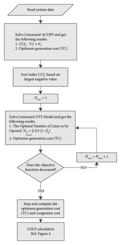
2. The Proposed Framework of OTS

The proposed framework of OTS problem shown in Figure 1 employs a linearized method of ACOPF equations. The algorithm starts by solving the linearized ACOPF model described in Section 3 and the linearized OTS is formulated as a MILP-OTS model (Section 4). To reduce the search space and calculation time of the OTS, a line ranking index called line congestion cost index (CCI) is used, which is illustrated in Section 4.2. The method of solving OTS problem is described as follows:

Step 1: a linearized ACOPF problem is applied on the power system.
Step 2: the congestion cost index (CCI_ij) is calculated for all transmission lines.
Step 3: a priority list of transmission lines is prepared by sorting their CCI_ij index based on the greatest negative value to the most positive value.
Step 4: the optimal lines to be disconnected is obtained by implementing the linearized OTS model for a certain maximum number of opening lines (N_max).
Step 5: Step 1– is repeated by increasing N_max in each iteration, if the objective function is not decreased with respect to its previous iteration.

Details are in the caption following the image — **Figure 1**
Open in figure viewer PowerPoint

The algorithm of the proposed optimal transmission switching.

3. The Linearized ACOPF Model

To model the TS problem, the integer programming method based on the ACOPF equations is used, and it plays an important role in the OTS problem. The main goal of the optimal power flow problem, which is a nonlinear programming (NLP) optimization, is to minimize the total generation cost of the power system while taking into account physical constraints such as transmission line flow limits, bus voltage limits, and the active and reactive power produced by power plants. ACOPF is classified as a nonconvex optimization problem because the active and reactive power flow equations are nonlinear. Consequently, a local optimal solution is obtained instead of a global one. For this purpose, many algorithms and solution methods were applied based on linearization to solve the abovementioned challenges at an acceptable speed [38, 39].

In the following, the linearization of ACOPF problem, including linearization of AC load flow equations and linearization of generators cost function is described.

3.1. Linearization of AC Power Flow Equations

In this section, the linear approximation of the AC load flow equations, is introduced. The basic load flow equations of a power system are given in the following:

()

where Equations (1) and (2) enforce the active and reactive power balances at each bus, respectively. Active (P_ij) and reactive (Q_ij) power flows in line (i.j) are presented in Equations (3) and (4), respectively.

: the active power generation in bus i.
: the reactive power generation in bus j.
: the amount of active load in bus i.
: the amount of reactive load in bus i.
|V_i|: the magnitude of voltage in bus i.
θ_ij: voltage angle difference between bus i and j(θ_ij = θ_i − θ_j)
g_ij: the series conductance in line (i.j).
b_ij: the series susceptance in line (i.j).
: the total shunt capacitive susceptance in the line (i.j).
N: the total number of buses in the system.
sb: slack bus.

There are several nonlinearity terms in above equations, namely, squared voltages, sine and cosine functions, and multiply variable by variable. The following assumptions are used to linearize AC power flow equations:

1.
Because in real power systems, the angle difference across a transmission line is small so that it is assumed that sin(θ_ij) ≈ θ_ij.
2.
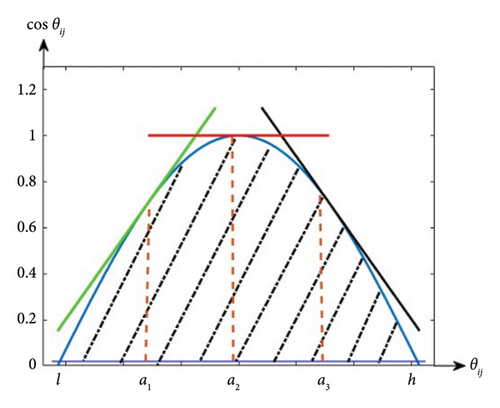
Linear piecewise method is used for the cosine function considering that it is convex in the range of −1.5–1.5 radians. Therefore, it is possible to determine the area of the acceptable solution according to Figure 2 by helping linear segments. In this model, the cosine function is considered in the range [l, h] and n_s line segments are selected on this function. Figure 2 depicts the assumption that the cosine function is partitioned into three distinct line segments, each of which is tangential to the cosine curve. Inequalities may be derived by considering the tangent lines at various places along the function. The dotted lines are the linear inequality constraints and thus the shaded area is the feasible region of the linear system formed by those constraints. For transmission line i-j, mathematical equations related to linear piecewise are obtained based on Equation (5). Furthermore, since the values of the cosine function are between zero and one, an equation related to the horizontal axis of the function is obtained by Equation (6) [40].
()

()
where
: a decision variable capturing the approximate value of cos θ_ij
n_s: the number of linear pieces of the cosine function
l: the lower limit of the argument of cosine function
h: the upper limit of the argument of cosine function
a_K: a point on the axis θ where the line segment is tangent to the cosine function at this point.

In this article, Equations (5) and (6) are shown with the expression .

Considering the above assumptions, the active and reactive power will be as follows:

()

Equations (7) and (8) are still nonlinear due to the multiplication of variables |V_i| and |V_j|. To linearize these equations, it is assumed that the bus voltages of power grid are within a standard variation range, and thus Equation (9) can be written as follows:

()

where

The selection of a value for the target voltage at each bus is purely hypothetical and should only be within the standard range of permissible voltages in the power system.

By replacing Equation (9) in Equations (7) and (8), the following equations for active and reactive power will be obtained.

()

After simplifying,

()

Equations (11) and (12) can be divided into the following two parts:

()

where

()

Considering

and ∆V_i∆V_j in Equations (16) and (17), they are nonlinear and after linearizing them using the Taylor series, and ignoring the second and higher degrees, the following equations will be obtained:

()

3.2. Cost Function Linearization

In the previous section, AC power flow equations were linearized and in this section, the cost objective function of the ACOPF is linearized. In general, the cost function of generators is assumed to be a quadratic function that is presented in the following equation for the i th generating unit [41].

()

The total generation cost (TC) of the power system is calculated as follows:

()

where

is the active power generation of the i th generating unit, N_g is the total number of generators, and

, and

are the constant parameters of the i th cost function.

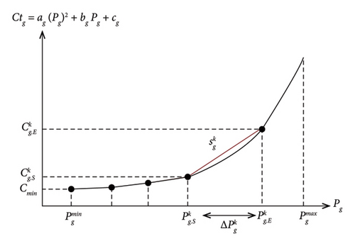
A piecewise linear interpolation method depicted in Figure 3 was applied to linearize the quadratic cost function of generators [42].

As shown in Figure 3, the distance between the lower and upper capacity limits of the generating unit (

and

) is divided into n linear segments with length

that is calculated in Equation (21). In kth interval [

, a variable

is defined that varies from zero to

according to Equation (22). The starting and ending points of kth interval on the horizontal axis (

and

) are calculated from Equations (23) and (24), respectively. For each generator and linear segment, the slope of offer curve is calculated to determine the resulting cost coefficient. Therefore, the starting point and the ending point of the kth interval related to the cost coefficients (

and

) are calculated from Equations (25) and (26), respectively. The slope of kth segment (

) is calculated in Equation (27). The aggregation of all the segments for power and the linearized cost function of generation g determined in Equations (28) and (29), respectively.

()

4. Problem Formulation

In this section, using the linearized model of the ACOPF equations explained in the previous section, a linearized model for solving the OTS problem is presented. The presented model determines how many transmission lines should be opened under certain power system loading conditions to impose the lowest operating cost on the system. Also, to consider the congestion of transmission lines in solving the problem, an index based on the congestion cost of transmission lines for line exit is used, the calculation method of which is described in this section. At the end of this section, the LOLP index is used by the MCS method to evaluate the reliability of the power system before and after switching.

4.1. Mathematical Model of Linearized OTS

To model the OTS problem, a binary variable z_ij indicating whether the transmission line is open or closed is applied in the linearized ACOPF equations. z_ij is equal to zero (z_ij = 0) if line (i.j) is isolated from the system (open) or z_ij = 1 if it is connected (closed). The objective function of the OTS problem is obtained from the linear combination of the objective function related to the linearization of AC power flow equations and the linearized objective function of the generation cost, which is equated with a coefficient β. This coefficient can be assumed based on the solution of the basic problem of AC power flow and the value of the objective function of solving ACOPF problem. The generation cost function in the ACOPF (OF₁ in Equation (31)) should be minimized and on the other hand the objective function related to the linearization of the cosine function in the AC power flow should be maximized (OF₂ in Equation (33)); therefore, in the final objective function (Equation (30)), the coefficient β with a negative sign should be used. The following equations are the linearized model of the OTS problem:

()

where

()

Equation (30) is the objective function of OTS problem. The Constraints (31)–(34) is the set of equations for linearizing the cost function of generators (Section 3.2). Constraints (35) and (36) are known as balancing constraints because they are determined by Kirchoff’s rules at each node and describe how power flows throughout the system. These constraints show that the amount of power flowing into a node equals the amount flowing out of the node. Equations (37)–(44) denote the active and reactive power flow on line (i.j) which is linearized according to Section 2.2. In these equations, M is called the “big M” value, which is sufficiently a big positive value to make the constraint nonbinding when z_ij is zero. The big M value can be determined by acknowledging that the transmission line must be returned to service at a later time stage and it is not desired to allow for the connecting buses to have a large angle separation; thus, M must be a large number greater than or equal to |b_ijθ^max − θ^min|. b_ij is the series susceptance of the transmission line (i.j). The min and max bus angle values are chosen ± 0.6 radians [43, 44]. Equation (45) is the set of equations regarding the linearization of the cosine function, which are obtained for each transmission line of the system based on Section 3.2. The active and reactive power of each generator is limited by Equations (47) and (48), respectively. Equation (49) shows the limitation of the cosine function. All bus voltages should be within the standard permissible range (50). Constraint (51) shows the voltage angle limitation in buses. Equations (52) and (53) impose the thermal limit of transmission lines, and Equation (54) limits the number of lines that are allowed to be switched. In this constraint, N_max is the maximum number of lines allowed to be switched and N_g is the number of generator buses.

OTS should not change the reliability of the system. Therefore, two Constraints (55) and (56) are considered for this purpose. First, since it is difficult to reconnect the power system after islanding and synchronizing of the system may lead to equipment failures, any OTS solution that leads to the system islanding will not be acceptable. Therefore, Constraint (55) prevents the system from being islanded in the OTS problem. ω is a set of transmission lines so that the power system would be islanded if all the lines in ω are opened. Constraint (55) ensures that in any solution, all lines in set ω are not opened. Now, if there are several sets of ω, then Ω is defined as a whole set containing all the ω. Second, the number of lines connected to each bus is restricted to two or more in order to ensure system reliability at a respectable level after TS. In other words, if one of the two interconnected lines is selected to be opened in the OTS problem, the reliability of the bus with just two lines connected significantly diminishes. To avoid this issue, Constraint (56) makes that at least two lines are connected to each bus within the solution OTS problem. K_i is the set of lines connected to bus i.

4.2. The Priority List Method in the OTS Problem

To reduce the solution time of OTS problem, priority lists of transmission lines that are candidates for switching were introduced using different criteria in previous studies. Some of these criteria are the power flow violation of transmission lines, the cost of line congestion, and the sensitivity of energy production cost to the lines’ power flow [45, 46]. In the following section, the congestion cost criterion is presented.

The congestion cost of transmission lines is defined as an increase in the production cost of generators due to the transmission constraints enforcement [47, 48]. To reduce the search space and calculation time of the OTS problem, a line ranking index called lineCCI (57) has been proposed in [49] based on dual variables of the OPF constraints.

()

where π_i and π_j are marginal prices of bus i and j, respectively, that are calculated based on the dual variables of the power balance Constraint (35) by the linearized ACOPF model presented in this paper. The idea in [48] suggested that the most negative CCI_ij is likely to show the most promising line removal for having the largest cost reduction. After calculating CCI_ij for each line, the obtained values are sorted according to the largest negative value. The obtained list will be the priority list of transmission line switching candidates. By opening the transmission line that has the most negative value, the greatest reduction in the generation cost of the power system will be obtained.

4.3. Probabilistic Reliability Calculation

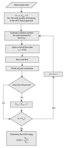
To evaluate reliability of the system in the OTS, the LOLP index has been calculated in two states: pre- and postswitching for different numbers of opening lines. The Monte Carlo Simulation (MCS) method is used to calculate the LOLP index of the system. In each iteration of MCS, random numbers are generated for all the transmission lines first and then lines with the random number greater than the outage rate are selected as contingency. By executing an optimal power flow in each iteration, it is determined whether loss of load occurs or not. The LOLP index is calculated based on the ratio of number of iterations that the load is not supplied to the total number of iterations [28]. The flowchart of the MCS-based method shown in Figure 4 is used to calculate the approximate value of the LOLP reliability index for a power system topology, which is determined by solving the OTS problem.

5. Simulation Results

5.1. Validation of the Proposed Linearized ACOPF

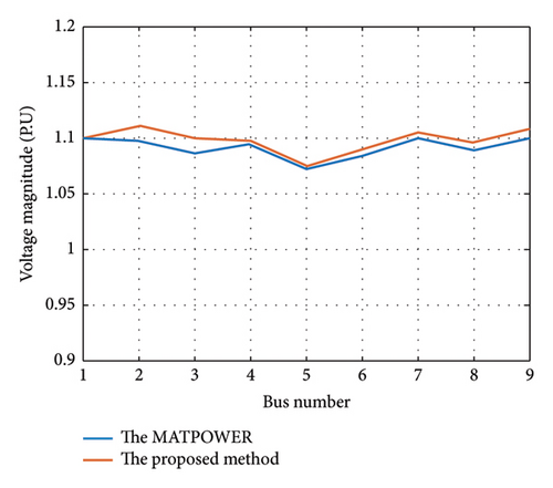
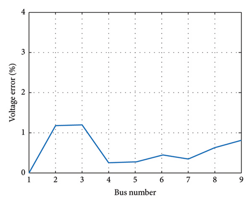
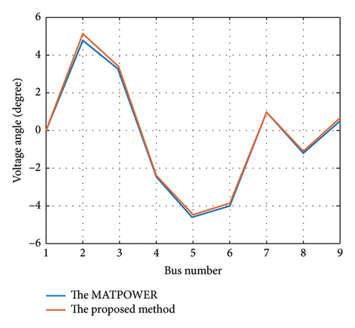
The proposed model was applied to two standard test systems: the 9-Bus test system and IEEE 118-bus using GAMS software. First, the accuracy of linearized ACOPF is evaluated on an IEEE 9-bus test system whose single-line diagram is shown in Figure 5 [50]. The obtained results of the linearized ACOPF are compared with ACOPF by MATPOWER [51]. Figures 6 and 7 illustrate the voltage magnitude and its percentage error between the proposed linearized ACOPF and the nonlinear ACOPF via MATPOWER. As can be seen from Figure 5, the error is less than 1.5% on each bus and its average is equal to 0.6%. Figure 8 presents a comparison among the voltage angles obtained by the proposed model and MATPOWER. The average error in this case is 0.14°. It is observed that the obtained results in voltage magnitude and angles have appropriate approximation with MATPOWER results. Table 1 presents the output power of the generators by the proposed method and MATPOWER.

Table 1. Active power of generators and objective function in two linear and nonlinear methods.

Items	The results obtained from MATPOWER	The results obtained from the proposed method
	89.8	89.2
	134.32	134.7
	94.19	94.38
Objective function ($/h)	5296.69	5296.01

5.2. Optimal Transmission Line Switching at IEEE 118-Bus

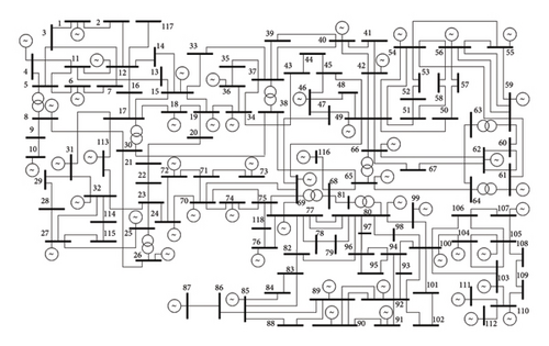
To show the effect of OTS on the reduction of congestion, and generation cost, three scenarios are defined and analyzed on the IEEE 118-bus system whose single-line diagram is shown in Figure 9. The test system comprises 118 buses, 186 transmission lines, 19 generating units, and 99 load buses [52–54]. The studied scenarios are three different load levels. Scenarios I–III are defined by multiplying the load level (base case) presented in [52] by the values of 1, 0.8, and 1.2, respectively. Consequently, the total load in three situations is 4242 MW, 3818 MW, and 5090 MW, respectively. In addition, there are 100-line pieces in the linearization of the cost function and the cosine function.

In Scenario I, a load profile which is presented in [52] is studied as the base case. Using the proposed linearized ACOPF, total generation and congestion cost is determined 138,362 ($/h) and 12,060 ($/h) before switching, respectively. The CCI_ij is calculated for all the transmission lines using Equation (57), and Table 2 shows the 20 lines with high removal priority that have the most negative CCI_ij values.

Table 2. The results of CCI_ij for the IEEE 118-bus system at Scenario I.

Rank number	Sending bus	Receiving bus	CCI_ij
1	25	26	−27.4643
2	5	8	−15.3817
3	43	44	−5.07155
4	56	58	−2.36323
5	32	113	−2.13629
6	11	12	−2.08441
7	85	89	−1.29523
8	60	62	−0.5699
9	61	64	−0.5488
10	77	78	−0.50817
11	55	56	−0.4451
12	19	34	−0.43512
13	109	110	−0.39314
14	19	20	−0.34604
15	108	109	−0.19251
16	34	36	−0.03374
17	70	71	−0.02424
18	114	115	−0.00394
19	35	36	0.00471
20	71	73	0.01785

From the priority list, the top 40 transmission lines were selected as candidates for the opening. The results of changing a maximum number of switching, N_max in Equation (54), on the total generation and congestion cost are presented in Table 3. It is found by trial and error that choosing the N_max more than 7 does not affect reducing the objective function. It is evident that when a maximum of seven transmission lines is disconnected, the values of congestion and total generating cost reach their minimal values and stay there. This means that even by choosing N_max greater than 7, the optimal number of switching will be equal to 7. The total generation cost will decrease by 828 ($/h), and the total congestion cost will decrease by 1275 ($/h) with the opening of 7 transmission lines.

Table 3. Total generation and congestion cost for the IEEE 118-bus system at Scenario I with OTS.

Maximum number of open lines allowed	The optimal number of lines to be opened	Generation cost ($/h)	Congestion cost ($/h)	Reduction in congestion cost compared with before switching ($/h)	Reduction in generation cost compared with before switching ($/h)
0	0	138,362	12,060	0	0
1	1	137,609	10,975	1085	753
2	2	137,579	10,867	1193	783
3	3	137,555	10,795	1265	807
4	4	137,547	10,852	1208	815
5	5	137,542	10,867	1193	820
6	6	137,536	10,805	1255	826
7	7	137,534	10,785	1275	828
8	7	137,534	10,785	1275	828
9	7	137,534	10,785	1275	828

In the second scenario, a new load level is assumed by multiplying the demand of main power system by 0.8. Given that in Scenario II, the system load level is low, so the congestion of transmission lines is little and switching will have less impact on decrease of total generating and congestion costs. In this load scenario, by opening the number of 5 transmission lines, the global optimal solution in the OTS problem is obtained and the total cost of generation and congestion will decrease by 561 ($/h) and 545 ($/h), respectively.

To further investigate the effect of transmission line switching, OTS problem was solved in Scenario III, which has a higher amount of load than the previous two scenarios. Based on the results obtained from solving the OTS problem for load Scenario III, the total generation and congestion cost will decrease by 3043 ($/h) and 15,530 ($/h), respectively, after OTS. The results indicate that in Scenario III, which has a load level 20% higher than the base case, establishing 8 transmission lines would result in a reduction of about 27% in the overall congestion cost of the system. Table 4 shows the optimal results of solving the OTS problem in three different Scenarios I–III. In this table, for each load scenario, the optimal number of lines to be opened, the lines to be opened, and the total generation and congestion cost in two states before and after TS are presented.

Table 4. Total generation and congestion cost of the IEEE 118-bus system in three different Scenarios I–III.

Scenarios	The optimal number of lines to be opened	Lines to be opened	Total generation cost ($/h)		Total congestion cost ($/h)
Scenarios	The optimal number of lines to be opened	Lines to be opened	Pre-OTS	Post-OTS	Pre-OTS	Post-OTS
I	7	(11–12), (25–26), (19–34), (43–44), (55–56), (61–64), (77–78)	138,362	137,534	12,060	10,785
II	5	(11–12), (25–26), (43–44), (61–64), (94–95)	101,973	101,412	6482	5937
III	8	(11–12), (25–26), (19–34), (47–49), (60–62), (75–77), (76–77), (88–89)	184,143	181,100	56,843	41,313

Based on the results presented in Table 4, the lines that should be opened are the ones with the highest negative value of CCI from the priority list which will have the greatest impact on reducing of generation and congestion costs. The lines with the positive values in the priority list were opened in order to look into this matter. After doing an ACOPF, it was found that the expenses associated with generation and congestion had not only decreased but significantly risen in comparison to the preswitching period.

Furthermore, in the low load scenario (Scenario II with 80% of the baseload), a few number of lines are opened because the system congestion is low, while in heavy load conditions, more are opened due to high congestion. The important advantage of the proposed method compared with the others is that it is completely a linear method which is not based on the various assumptions of DCOPF method at the same time. It can be confidently claimed that the solution obtained from the optimization problem is a global optimal solution.

Figures 10 and 11 show the reduction of the total generation and congestion cost according to the maximum number of lines that are allowed to be opened in Scenario III.

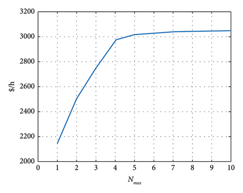
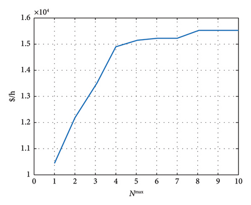
Figures 10 and 11 demonstrate that increasing the maximum number of allowable open lines (N_max) leads to cost reduction. If N_max exceeds a certain threshold (e.g., greater than 8 in the third scenario), the reduced costs associated with generation and congestion costs remain at a fixed value. Consequently, in the linearized OTS method, the optimal number of open lines becomes a unique and fixed value. This is one of the advantages of linear method of OTS, which is introduced in this article. This is in the case that in the nonlinear method, parameter N_max cannot be chosen with certainly in such a way as to reach the optimal solution because despite the fact that the problem is apparently optimized in a state of solving the problem with a certain parameter of N_max, if it increases again. This parameter may find better optimal solutions. Therefore, in the nonlinear method, there is no clear scenario to claim that the solution is optimal.

5.3. Effects of TS on LMPs

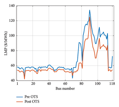
From the viewpoint of LMP, the simulation results were analyzed and the values of LMPs were compared in two states before and after switching. Because in load Scenarios I and II, congestion of lines happens less; therefore, the values of LMPs before and after switching do not differ significantly. Figure 12 shows the LMP changes for Scenario III before and after switching. Table 5 shows the minimum, maximum, and average values of LMP before and after switching the transmission lines for different load scenarios in the IEEE 118-bus system.

Table 5. Minimum, maximum, and average value of LMPs in different load scenarios.

Scenario	Min LMP ($/MWh)		Max LMP ($/MWh)		Avg. LMP ($/MWh)
Scenario	Pre-OTS	Post-OTS	Pre-OTS	Post-OTS	Pre-OTS	Post-OTS
I	41	40	53.5	52.6	45.7	45.2
II	36.8	36.7	43.8	43.5	39.9	39.7
III	42	42	134.3	124.9	71.2	62.9

As can be seen from Table 5, in the Scenarios I and II, the LMP values before and after switching do not change, while in Scenario III, which has a higher load level than other two scenarios, the average LMP value of the system is from 71.2 ($/MWh) to 61.9 ($/MWh) has decreased, which indicates the reduction of congestion and related costs after switching.

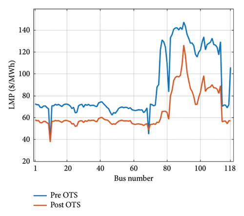
In the third scenario, the effect of the OTS problem in reducing the total generation and congestion cost are investigated by altering the maximum flow of the transmission lines that have the highest congestion cost. Based on the data obtained from the ACOPF issue prior to the switching, it has been noted that the transmission line connecting buses 9 and 10 exhibits the largest congestion cost, as well as a significant power flow. It is assumed that maximum power flow of this line is changed from 500 to 400 MVA and the OTS problem of OTS is solved in this scenario. The optimal solution depicted in Table 6 illustrates that by opening 6 transmission lines, the total generation and congestion cost decreased from 186,119 $/h to 182,286 $/h, which was reduced by 3833 $/h. Besides, the total congestion cost decreased from 81,329 $/h to 44,197 $/h, which has decreased by 37,132 $/h, which is about 45%. Table 7 shows the results of LMP in two states before and after switching. Based on the results of this table, the average value of LMP has decreased by 23 ($/MWh), which is about 26%. Applying OTS specially in periods of high load demand can significantly reduce the costs of generation and congestion. Figure 13 shows the changes of LMP for all the busses of the system, as well as for the busses that have a greater reduction in LMPs compared with before switching, respectively. As can be seen from these figures, in conditions of high system congestion, the switching of transmission lines will have a significant reduction in LMPs.

Table 6. Total generation and congestion cost in Scenario III by changing the power limit of lines 9-10.

The optimal number of lines to be opened	Lines to be opened	Total generation cost ($/h)		Total congestion cost ($/h)
The optimal number of lines to be opened	Lines to be opened	Pre-OTS	Post-OTS	Pre-OTS	Post-OTS
6	(25–26), (32–113), (47–49), (75–77), (76–77), (88–89)	186,119	182,286	81,329	44,197

Table 7. Minimum, maximum, and average LMP values in Scenario III by changing the power limit of line 9-10.

Min LMP ($/MWh)		Max LMP ($/MWh)		Avg. LMP ($/MWh)
Pre-OTS	Post-OTS	Pre-OTS	Post-OTS	Pre-OTS	Post-OTS
37	37	147	126	88	65

5.4. Effects of TS on System Reliability and Security

Changing the power system topology by OTS may affect the reliability. Equations (55) and (56) are considered as reliability requirements: the first one prevents the power system from islanding, while the second guarantees that at least two lines are connected to each bus so that the reliability of the system is not damaged due to the fault occurrence for one of these lines. In the following, the reliability of system before and after TS for the IEEE 118-bus system is analyzed.

5.4.1. LOLP Reliability Index

To evaluate the reliability of system in the OTS, the LOLP index was calculated in two states: pre- and postswitching for different numbers of opening lines. MCS method is used to calculate the LOLP index of the system [28]. All transmission lines are considered to have an outage rate of 0.01 outage/km/year in this research. By taking into account 100,000 samples, the LOLP index is converged to a value that is roughly constant. The LOLP values for pre and after switching in Situations I through III are shown in Table 8. The index is obtained as 3.45%, 3.33%, and 4.54% before TS for Scenarios I–III, respectively. The results of Scenario III (heavy load) depict that after opening 2 transmission lines, the LOLP index is equal to 4.81%, which has not changed significantly compared to pre-OTS (4.54%). However, if the number of switching increases more than 3 lines, the LOLP index increases and in the optimal solution of the OTS problem (opening 8 lines), this index increases to 6.75. It is reminded that according to Table 4 of the article, the optimal number of OTS in Scenarios I–III are 7, 5, and 8, respectively.

Table 8. The LOLP index before and after optimal transmission switching in Scenarios I–III.

	The number of lines to be opened	The LOLP index (%)
	The number of lines to be opened	Scenario I (base case)	Scenario II (80% of base case)	Scenario III (120% of base case)
Pre-OTS	0	3.45	3.33	4.54

Post-OTS	1	4.02	3.62	4.75
	2	4.25	3.89	4.81
	3	4.90	4.78	5.56
	4	5.70	5.41	6.03
	5	5.84	5.73	6.10
	6	5.96	—	6.48
	7	6.45	—	6.56
	8	—	—	6.75

5.4.2. Contingency Analysis

To further investigate the security of system after transmission line switching, an N-1 contingency analysis is studied in this section to determine whether the system after OTS can withstand the loss of one more element (line disconnecting) as a contingency. Before and after the switching of transmission lines, the N-1 contingency analysis was conducted by disconnecting each transmission line and counting the number of instances in which the system security constraints (line capacity, bus voltage, and not supplied load) are violated. Table 9 shows the results of N-1 contingency analysis for different numbers of TS in Scenarios I–III. After switching of transmission lines, the number of cases that violate security constraints slightly increased and the ratio of unsuccessful cases to the total number of contingencies has increased from 6.45% before TS to 10.11% afterTS in Scenario III. Thus, the N-1 contingency is affected slightly by TS.

Table 9. The results of N − 1 contingency analysis for different number of transmission switching in Scenarios I–III.

	The number of lines to be opened	The number of rejected cases in contingency analysis			The ratio of the rejected cases to the total cases (%)
	The number of lines to be opened	Scenario I	Scenario II	Scenario III	Scenario I	Scenario II	Scenario III
Pre-OTS	0	10	9	12	5.38	4.84	6.45

Post-OTS	1	11	10	14	5.94	5.40	7.56
	2	11	10	14	5.98	5.43	7.60
	3	13	11	16	7.10	6.01	8.74
	4	15	13	17	8.24	7.14	9.34
	5	15	13	17	8.29	7.18	9.39
	6	16	—	17	8.88	—	9.44
	7	16	—	18	8.94	—	10.05
	8	—	—	18	—	—	10.11

Despite the obtained results, which show that the LOLP and N-1 contingency analysis is affected by TS, it should be noted that the power network is a very complex system so that various factors, such as the power system topology, generators’ dispatch, available capacity of generators, ramp rate of generators, and system load, affect the reliability of the system. It is often thought that opening the transmission line reduces the reliability of the system. In general, the temporary opening of a transmission line does not necessarily reduce the reliability of the system. The essential issue is whether the system can still satisfy the given reliability criteria after switching the transmission lines, not if the reliability of the system reduces after transmission change. Furthermore, the goal of system operator is to operate the power system with the minimum cost subject to the system’s security constraints and to meet the system’s reliability requirements. If there are two generation dispatch schedules and both schedules meet both the reliability requirements and the load flow constraints, the system operator prefers to choose the solution that costs less [1, 55].

5.5. Comparison of the Proposed Method With the Nonlinear One

To have a precise evaluation, a comparison was made between the proposed linearized AC OPF and the nonlinearized one [56] with the same model (objective and constraints). GAMS software was used to implement the transmission line switching utilizing nonlinear optimum power flow issue that was reported in [56, 57]. The IEEE 118-bus test system was used to apply this model using the reference data found in [52]. Table 10 shows the results of the TS through nonlinear OPF for Scenarios I–III, which are baseload, 80% of baseload, and 120% of baseload, respectively.

Table 10. The results of the transmission switching through nonlinear OPF in three scenarios.

Scenario	The optimal number of lines to be opened	Lines to be opened	Total generation cost ($/h)		Total congestion cost ($/h)
Scenario	The optimal number of lines to be opened	Lines to be opened	Pre-OTS	Post-OTS	Pre-OTS	Post-OTS
I	8	(11–12), (19–20), (60–56), (60–62), (85–89), (61–64), (77–78), (109–110)	138,362	137,627	12,060	11,960
II	1	(25–26)	101,973	101,941	6482	6419
III	8	(11–12), (74–75), (17–113), (47–49), (60–62), (75–77), (76–77), (77–88)	184,143	181,936	56,843	43,772

Table 11 compares the reduction of total generation and congestion cost in nonlinear and linear (proposed method) TS. In the nonlinear OTS, a significant cost reduction is not achieved, and the global optimal solution is not guaranteed as well due to the nonlinear nature of the problem. In addition, in this method and Scenario II, which accounts for 80% of the base load, include the selection of just one transmission line for switching. As a result, the generation costs have decreased by 32 $/h and the congestion costs have decreased by 63 $/h. However, in the linearized OTS method proposed in this paper, five lines have been selected for switching in Scenario II, and the generation and congestion costs have been reduced by 561 $/h and 545 $/h, respectively.

Table 11. The results of the nonlinear-based OTS method vs. the proposed linearized OTS.

Scenarios	The optimal number of lines to be opened		Reduction in total generation cost ($/h)		Reduction in total congestion cost ($/h)
Scenarios	NL-OTS	Proposed method	NL-OTS	Proposed method	NL-OTS	Proposed method
I	8	7	735	828	100	1275
II	1	5	32	561	63	545
III	8	8	2207	3043	13,071	15,530

By comparing these two methods, the linearized OTS method has a large reduction in costs compared with the nonlinear one. On the other hand, one of the most important advantages of the linearized OTS is having a unique answer and reaching to the global optimal solution, while in the nonlinear method, different solutions may arise each time the program is executed due to the existence of locally optimal solutions.

The computational time of the linearized OTS problem proposed in this paper is about 1 minute or less. A computer Intel (R) Core (TM) i5-4200 CPU @ 2.3 GHz with 6 GB RAM is deployed for the computations. The linearization method of OTS problem presented in this paper has significantly reduced the calculation time of solving the problem compared with the nonlinear method, while the problem will lead to a globally optimal solution.

6. Conclusion

In this paper, we propose a fully linearized ACOPF model to address the issue of OTS. The study aims to minimize generation and congestion costs by altering the system topology through OTS as a corrective mechanism. Given the binary nature of switching variables, the ACOPF equations, and the typically nonlinear objective function, the TS problem is inherently highly nonlinear. To achieve a globally optimal solution while reflecting the real conditions of nonlinear power systems, we employ an AC TS model that is fully linearized using a combination of linearization techniques. Initially, the proposed linearized ACOPF model was tested on a 9-bus system, demonstrating high accuracy across various system parameters. By incorporating binary switching variables into the linearized ACOPF, we developed the linearized OTS model, which was subsequently applied to the IEEE 118-bus system under different load scenarios. The results indicate that opening lines with the most negative CCI significantly reduces generation and congestion costs, and conversely, the lines with the least negative impact should be prioritized for closure.

Moreover, the combination of TS and generation rescheduling leads to a decrease in LMPs and overall congestion costs in the system. A key concern for system operators, particularly during peak loads, is maintaining system reliability post-TS. To assess reliability, we calculated the LOLP index using the MCS method, evaluating the system’s reliability before and after the switching of lines. However, it is important to note that system reliability cannot be solely determined by network topology analysis. For example, TS may enable a more reliable generation dispatch solution. In addition, even if a line is opened during steady-state operation, a more intelligent and flexible system could reinstate these lines after a contingency occurs.

Looking ahead, we plan to explore the OTS problem further by considering the high penetration of renewable energy sources and the associated uncertainties.

Nomenclature

:: The active power generation in bus i
: The reactive power generation in bus j
: The amount of active load in bus i
: The amount of reactive load in bus i
P_ij: Active power flows in line (i.j)
Q_ij: Reactive power flows in line (i.j)
|V_i|: The magnitude of voltage in bus i
θ_ij: Voltage angle difference between bus i and j
g_ij: The series conductance in line (i.j)
b_ij: The series susceptance in line (i.j)
: The total shunt capacitive susceptance in the line (i.j)
N: The total number of buses in the system
N_g: The total number of generators
N_max: The maximum number of lines allowed to be switched
sb: Slack bus
: A decision variable capturing the approximate value of cos θ_ij
n_s: The number of linear pieces of the cosine function
l: The lower limit of the argument of cosine function
h: The upper limit of the argument of cosine function
a_K: A point on the axis θ where the line segment is tangent to the cosine function at this point
: Target voltage of bus i
, , and: The constant parameters of the i th cost function
z_ij: Binary variable indicating whether transmission line is removed from the system (open, z_ij = 0), or in the system (closed, z_ij = 1)
M: The “big M” value
: Maximum and minimum voltage angle in bus i
: Maximum and minimum magnitude of voltage in bus i
: Maximum and minimum active capacity of generator g
: Maximum and minimum reactive capacity of generator g
: Maximum capacity of line (i.j)
π_i: The marginal prices of bus i
CCI_ij: The line congestion cost index
N_LOL: The number of iterations with unserved load demand in the MCS-based approach
N_mo: The total number of iterations in the MCS-based approach
m: The iteration index of the simulation
FOR_k: The outage rate of the kth transmission line
γ_k: A random number for each transmission line (k)

Disclosure

A nonpeer-reviewed version of another manuscript entitled “A linearized AC optimal power flow model based on a piecewise linear approximation along with a Taylor series” has been presented as a preprint [58], available at Research Square preprint server (https://doi.org/10.21203/rs.3.rs-4019175/v1).

Conflicts of Interest

The authors declare no conflicts of interest.

Funding

The author received no specific funding for this work.

Open Research

Data Availability Statement

The data that support the findings of this study are available from the corresponding author upon reasonable request.

References

1 Hedman K. W., Oren S. S., and O’Neill R. P., A Review of Transmission Switching and Network Topology Optimization, IEEE General Meeting Power& Energy Society, 2011, San Diego, CA, 1–7.
Google Scholar
2 Fisher B., O’Neill P., and Ferris C., Optimal Transmission Switching, IEEE Transactions on Power Systems. (2008) 23, no. 3, 1346–1355.
10.1109/TPWRS.2008.922256
Web of Science® Google Scholar
3 Numan M., Abbas M. F., Yousif M., Ghoneim S. S. M., Mohammad A., and Noorwali A., The Role of Optimal Transmission Switching in Enhancing Grid Flexibility: A Review, IEEE Access. (2023) 11, 32437–32463.
10.1109/ACCESS.2023.3261459
Web of Science® Google Scholar
4 Anton H. and David P., Optimal Transmission Switching: Improving Solver Performance Using Heuristics, IEEE Transactions on Power Systems. (2023) 38, no. 4, 3317–3330.
Google Scholar
5 Jiang J., Wu H., Li W., Dong J., and Gu X., Economic Dispatch for Interconnected Power Network Considering Optimal Transmission Switching, 18th International Conference on AC and DC Power Transmission (ACDC 2022), Online Conference, 2022, China, 1307–1313.
Google Scholar
6 Pinzón S., Carrión D., and Inga E., Optimal Transmission Switching Considering N-1 Contingencies on Power Transmission Lines, IEEE Latin America Transactions. (2021) 19, no. 4, 534–541.
10.1109/TLA.2021.9448535
Web of Science® Google Scholar
7 Bugaje A. A. B., Cremer J. L., and Strbac G., Real-time Transmission Switching with Neural Networks, IET Generation, Transmission & Distribution. (2023) 17, no. 3, 696–705.
10.1049/gtd2.12698
Web of Science® Google Scholar
8 Behnia H. and Akhbari M., Integrated Generation and Transmission Maintenance Scheduling by Considering Transmission Switching, International Transactions on Electrical Energy Systems. (2019) 29, no. 4.
10.1002/etep.2792
Web of Science® Google Scholar
9 Numan M., Feng D., Abbas F., Rahman U., and Wattoo W. A., Impact Assessment of a Co-Optimized Dynamic Line Rating and Transmission Switching Topology on Network Expansion Planning, International Transactions on Electrical Energy Systems. (2020) 30, no. 8.
10.1002/2050-7038.12457
Web of Science® Google Scholar
10 Fattahi S., Lavaei J., and Atamtürk A., A Bound Strengthening Method for Optimal Transmission Switching in Power Systems, IEEE Transactions on Power Systems. (2019) 34, no. 1, 280–291.
10.1109/TPWRS.2018.2867999
Web of Science® Google Scholar
11 Xuan L., Yunfeng W., and Zuyi L., Multiple Solutions of Transmission Line Switching in Power Systems, IEEE Transactions on Power Systems. (2018) 33, no. 1, 1118–1120.
10.1109/TPWRS.2017.2770019
Google Scholar
12 Boshi Z., Zechun H., Qian Z., Hongcai Z., and Yonghua S., Optimal Transmission Switching to Eliminate Voltage Violations during Light-Load Periods Using Decomposition Approach, Journal of Modern Power Systems and Clean Energy. (2019) 7, no. 2, 297–308.
10.1007/s40565-018-0422-4
Google Scholar
13 Yang B., Yong F., H aiwang Z., Qing X., and Chongqing K., A Two-Level Approach to AC Optimal Transmission Switching with an Accelerating Technique, IEEE Transactions on Power Systems. (2017) 32, no. 2, 1616–1625.
Google Scholar
14 Khodaei A. and Shahidehpour M., Security-constrained Transmission Switching with Voltage Constraints, Electrical Power and Energy Systems. (2012) 35, 74–82.
10.1016/j.ijepes.2011.09.014
Web of Science® Google Scholar
15 Khodaei A. and Shahidehpour M., Transmission Switching in Security-Constrained Unit Commitment, IEEE Transactions on Power Systems. (2010) 25, no. 4, 1937–1945.
10.1109/TPWRS.2010.2046344
Web of Science® Google Scholar
16 Gong L., Wang C., Zhang C., and Fu Y., High-Performance Computing Based Fully Parallel Security-Constrained Unit Commitment with Dispatchable Transmission Network, IEEE Transactions on Power Systems. (2019) 34, no. 2, 931–941.
10.1109/TPWRS.2018.2876025
Web of Science® Google Scholar
17 Han T., Hill D. J., and Song Y., Optimal Transmission Switching with Uncertainties from Both Renewable Energy and N-K Contingencies, IEEE Transactions on Sustainable Energy. (2023) 14, no. 4, 1964–1978, https://doi.org/10.1109/TSTE.2023.3278072.
10.1109/TSTE.2023.3278072
Web of Science® Google Scholar
18 Lam L. H., Nam L. K., and Hieu N. H., Multi-Period Transmission Switching Strategy Analysis Considering Thermal Unit Commitment, Advances in Electrical and Computer Engineering. (2023) 23, no. 1, 51–60, https://doi.org/10.4316/AECE.2023.01006.
10.4316/AECE.2023.01006
Web of Science® Google Scholar
19 Li R., Ye P., Jiang D., Ma L., and Sun C., Optimal Transmission Switching for Power System Integrating Renewable Energy Based on Analytical Target Cascading, Frontiers in Energy Research, 11, https://doi.org/10.3389/fenrg.2023.1239232.
10.3389/fenrg.2023.1239232
Google Scholar
20 Thomas L., Leonard K., Iwo B., and Lutz H., Solving Combined Optimal Transmission Switching and Optimal Power Flow Sequentially as Convexificated Quadratically Constrained Quadratic Program, Electric Power Systems Research, 212, no. 2022, https://doi.org/10.1016/j.epsr.2022.108534.
10.1016/j.epsr.2022.108534
Google Scholar
21 Numan M., Feng D., Abbas F., Habib S., and Rasool A., Mobilizing Grid Flexibility through Optimal Transmission Switching for Power Systems with Large-scale Renewable Integration, International Transactions on Electrical Energy Systems. (2020) 30, no. 3.
10.1002/2050-7038.12211
Web of Science® Google Scholar
22 Granelli G., Montagna M., Zanellini F., Bresesti P., Vailati R., and Innorta M., Optimal Network Reconfiguration for Congestion Management by Deterministic and Genetic Algorithms, Electric Power Systems Research. (2006) 76, no. 6-7, 549–556.
10.1016/j.epsr.2005.09.014
Web of Science® Google Scholar
23 Rahimi A. F. and Sheffrin A. Y., Sequential Analysis of Optimal Transmission Switching with Contingency Assessment, IET Generation, Transmission & Distribution. (2018) 12, no. 6, 1390–1396.
10.1049/iet-gtd.2017.0435
Google Scholar
24 Kumar Gupta A., Kiran D., and Abhyankar A. R., Flexibility in Transmission Switching for Congestion Management, IEEE 2016 National Power Systems Conference (NPSC), December 2016, Bhubaneswar, India, 1–5.
Google Scholar
25 Rolim J. G. and Machado L. J. B., A Study of the Use of Corrective Switching in Transmission Systems, IEEE Transactions on Power Systems. (1999) 14, no. 1, 336–341.
10.1109/59.744552
Web of Science® Google Scholar
26 Khanabadi M. and Ghasemi H., Transmission Congestion Management through Optimal Transmission Switching, 2011, IEEE Power and Energy Society General Meeting.
10.1109/PES.2011.6039357
Google Scholar
27 Han J. and Papavasilioua A., Congestion Management through Topological Corrections: A Case Study of Central Western Europe, Energy Policy. (2015) 86, 470–482.
10.1016/j.enpol.2015.07.031
Web of Science® Google Scholar
28 Salkuti S., Congestion Management Using Optimal Transmission Switching, IEEE Systems Journal. (2018) 1–10.
Web of Science® Google Scholar
29 Sheik M., Aghaei J., Rajabdorri M., Shafie-khah M., and Lotfi M., Multi Objective Congestion Management and Transmission Switching Ensuring System Reliability, IEEE International Conference on Environment and Electrical Engineering and 2019 IEEE Industrial and Commercial Power Systems Europe (EEEIC/I&CPS Europe), 2019.
Google Scholar
30 Khanabadi M., Fu Y., and Liu C., Decentralized Transmission Line Switching for Congestion Management of Interconnected Power Systems, IEEE Transactions on Power Systems. (2018) 33, no. 6, 5902–5912.
10.1109/TPWRS.2018.2838046
Web of Science® Google Scholar
31 Paul K., Niranjan K., and Agrawal S., Optimal Rescheduling of Real Power to Mitigate Congestion with Incorporation of Wind Farm Using Gravitational Search Algorithm in Deregulated Environment, International Journal of Renewable Energy Resources. (2017) 7, no. 4, 1731–1740, https://doi.org/10.20508/ijrer.v7i4.6245.g7214.
10.20508/ijrer.v7i4.6245.g7214
Google Scholar
32 Paul K., Cuckoo Search Algorithm for Congestion Alleviation with Incorporation of Wind Farm, International Journal of Electrical and Computer Engineering. (2018) 8, no. 6, 4871–4879, https://doi.org/10.11591/ijece.v8i6.
10.11591/ijece.v8i6
Google Scholar
33 Paul K., Modified Grey Wolf Optimization Approach for Power System Transmission Line Congestion Management Based on the Influence of Solar Photovoltaic System, International Journal of Energy and Environmental Engineering. (January 2022) 13, 751–767, https://doi.org/10.1007/s40095-021-00457-2.
10.1007/s40095-021-00457-2
Web of Science® Google Scholar
34 Kocuk B., Dey S. S., and Sun X. A., New Formulation and Strong MISOCP Relaxations for AC Optimal Transmission Switching Problem, IEEE Transactions on Power Systems. (2017) 32, no. 6, 4161–4170.
10.1109/TPWRS.2017.2666718
Web of Science® Google Scholar
35 Fattahi S., Lavaei J., and Atamtürk A., Promises of Conic Relaxations in Optimal Transmission Switching of Power Systems, 2017 IEEE 56th Annual Conference on Decision and Control (CDC), 2017, Melbourne, VIC, Australia, 3238–3245.
Google Scholar
36 Lu M., Nagarajan H., Yamangil E., Bent R., Backhaus S., and Barnes A., Optimal Transmission Line Switching under Geomagnetic Disturbances, IEEE Transactions on Power Systems. (May 2018) 33, no. 3, 2539–2550.
10.1109/TPWRS.2017.2761178
Web of Science® Google Scholar
37 Sun Y., Tian Z., Wu W. et al., Iterative Relaxation Solution for AC Optimal Transmission Network Reconfiguration Considering Bus Splitting, IET Generation, Transmission & Distribution. (2021) 15, no. 22, 3204–3214.
10.1049/gtd2.12252
Web of Science® Google Scholar
38 Kumari M. S. and Maheswarapu S., Enhanced Genetic Algorithm Based Computation Technique for Multi-Objective Optimal Power Flow Solution, International Journal of Electrical Power. (2010) 32, no. 6, 736–742.
10.1016/j.ijepes.2010.01.010
Web of Science® Google Scholar
39 Liang R., Tsai S., Chen Y. et al., Optimal Power Flow by a Fuzzy Based Hybrid Particle Swarm Optimization Approach, Electric Power Systems Research. (2011) 81, no. 7, 1466–1474.
10.1016/j.epsr.2011.02.011
Web of Science® Google Scholar
40 Coffrin C. and Van Hentenryck P., A Linear-Programming Approximation of AC Power Flows, INFORMS Journal on Computing. (2014) 26, no. 4, 1–22.
10.1287/ijoc.2014.0594
Web of Science® Google Scholar
41 Wood A. J. and Wollenberg B. F., Power Generation, Operation and Control, 1996, Wiley Press, New York, NY.
Google Scholar
42 Castillo A., Lipka P., Watson J.-P., Oren S. S., and O’Neill R. P., A Successive Linear Programming Approach to Solving the Iv-Acopf, IEEE Transactions on Power Systems. (July 2016) 31, no. 4, 2752–2763.
10.1109/TPWRS.2015.2487042
Web of Science® Google Scholar
43 Hedman W., Ferris C., O’Neill R., Fisher E., and Oren S., Co-Optimization of Generation Unit Commitment and Transmission Switching with N-1 Reliability, IEEE Transactions on Power Systems. (May 2010) 25, no. 2, 1052–1063.
10.1109/TPWRS.2009.2037232
Web of Science® Google Scholar
44 Abdi-Khorsand M., Sahraei-Ardakani M., and Al-Abdullah M., Corrective Transmission Switching for N-1-1 Contingency Analysis, IEEE Transactions on Power Systems. (MARCH 2017) 32, no. 2, 1606–1615.
Web of Science® Google Scholar
45 Wu J., Green R., Neuhoff K., and Newbery D., On Selection of Transmission Line Candidates for Optimal Transmission Switching in Large Power Networks, 2013, IEEE.
Google Scholar
46 Pourahmadi F., Jooshaki M., and Hosseini H., A Dynamic Programming-Based Heuristic Approach for Optimal Transmission Switching Problem with N-1 Reliability Criterion, 2016 International Conference on Probabilistic Methods Applied to Power Systems (PMAPS) IEEE, 2016.
Google Scholar
47 Ruiz A., Fosterand M., Rudkevich A., and Caramanis C., Tractable Transmission Topology Control Using Sensitivity Analysis, IEEE Transactions on Power Systems. (2012) 27, no. 3, 1550–1559.
10.1109/TPWRS.2012.2184777
Web of Science® Google Scholar
48 Fuller J. D., Ramasra R., and Cha A., Fast Heuristics for Transmission-Line Switching, IEEE Transactions on Power Systems. (2012) 27, no. 3, 1377–1386.
10.1109/TPWRS.2012.2186155
Web of Science® Google Scholar
49 Soroush M. and Fuller J. D., Accuracies of Optimal Transmission Switching Heuristics Based on DCOPF and ACOPF, IEEE Transactions on Power Systems. (2014) 29, no. 2, 924–932.
10.1109/TPWRS.2013.2283542
Web of Science® Google Scholar
50 Nguyen T. B. and Pai M. A., Dynamic Security-Constrained Rescheduling of Power Systems Using Trajectory Sensitivities, IEEE Transactions on Power Systems. (2003) 18, no. 2, 848–854.
10.1109/TPWRS.2003.811002
Web of Science® Google Scholar
51 Zimmerman R. and Gan D., Matpower: A Matlab Power System Simulation Package.
Google Scholar
52 https://matpower.org/docs/ref/matpower6.0/case118.html.
Google Scholar
53 Zimmerman R. D., Murillo-Sa´nchez C. E., and Thomas R. J., MATPOWER: Steady-State Operations, Planning and Analysis Tools for Power Systems Research and Education, IEEE Transactions on Power Systems. (2011) 26, no. 1, 212–219.
10.1109/TPWRS.2010.2051168
Web of Science® Google Scholar
54 Power Systems Test Case Archive, 2011, https://www.ee.washington.edu/research/pstca/index.html.
Google Scholar
55 Hedman K. W., Oren S. S., and Richard P. O. N., Optimal Transmission Switching: Economic Efficiency and Market Implications, Journal of Regulatory Economics. (2011) 40, 111–140.
10.1007/s11149-011-9158-z
Web of Science® Google Scholar
56 Potluri T. and Hedman K. W., Impacts of Topology Control on the ACOPF, IEEE Power and Energy Society General Meeting, 2012, San Diego, CA, 1–7, https://doi.org/10.1109/PESGM.2012.6345676, 2-s2.0-84870588870.
10.1109/PESGM.2012.6345676
Google Scholar
57 Khanabadi M., Ghasemi H., and Doostizadeh M., Optimal Transmission Switching Considering Voltage Security and N-1 Contingency Analysis, IEEE Transactions on Power Systems. (2013) 28, no. 1, 542–550, https://doi.org/10.1109/TPWRS.2012.2207464, 2-s2.0-84872846703.
10.1109/TPWRS.2012.2207464
Web of Science® Google Scholar
58 Habibi M. and Zanganeh A., A Linearized AC Optimal Power Flow Model Based on a Piecewise Linear Approximation along with a Taylor Series, Research Square, https://doi.org/10.21203/rs.3.rs-4019175/v1.
10.21203/rs.3.rs-4019175/v1
Google Scholar

All articles

Optimal Transmission Switching for Congestion Management and Cost Reduction Using Linearized AC Optimal Power Flow

Abstract