Nonintrusive Load Disaggregation Based on Attention Neural Networks
Abstract
Nonintrusive load monitoring (NILM), also known as energy disaggregation, infers the energy consumption of individual appliances from household metered electricity data. Recently, NILM has garnered significant attention as it can assist households in reducing energy usage and improving their electricity behaviors. In this paper, we propose a two-subnetwork model consisting of a regression subnetwork and a seq2point-based classification subnetwork for NILM. In the regression subnetwork, stacked dilated convolutions are utilized to extract multiscale features. Subsequently, a self-attention mechanism is applied to the multiscale features to obtain their contextual representations. The proposed model, compared to existing load disaggregation models, has a larger receptive field and can capture crucial information within the data. The study utilizes the low-frequency UK-DALE dataset, released in 2015, containing timestamps, power of various appliances, and device state labels. House1 and House5 are employed as the training set, while House2 data is reserved for testing. The proposed model achieves lower errors for all appliances compared to other algorithms. Specifically, the proposed model shows a 13.85% improvement in mean absolute error (MAE), a 21.27% improvement in signal aggregate error (SAE), and a 26.15% improvement in F1 score over existing algorithms. Our proposed approach evidently exhibits superior disaggregation accuracy compared to existing methods.
1. Introduction
Facing the energy shortage problem, all countries actively carry out energy transformation, energy preservation and emission reduction. As one of the major energy consumers, households are significant to energy conservation and the emission reduction. To accomplish this, the nonintrusive load monitoring (NILM) was proposed by Hart [1] in 1992. Its aim is to extract the energy usage of each household appliance using main meter data. In [2, 3] the authors show that feeding the disaggregated information to residential users can reduce their energy consumption by about 15%. NILM can reduce customers’ power consumption by improving their behaviors [4], and help grid operators provide different and precise services [5]. During the past several years, the NILM study has attracted much attention with the smart grid development.
Now, there is a behind-the-meter (BTM) system [6] that involves integrated energy storage systems, such as batteries, allowing users to store excess electricity for future use. This approach, highlighted in emerging markets such as data centers, aims to address peak demand costs, enhance grid stability, and provide backup power during outages in regions with unreliable power grids. Residential households can have PV, BESS, and EV charging infrastructures in their site and they have more complex load profiles, so it could be more challenging for the NILM process, making the disaggregation problem even harder to solve [7]. Therefore, efficient and intelligent load monitoring technology is more needed to analyze residential electricity consumption data.
In recent years, scholars have used Appliance Level Energy Character extraction (ALEC) to extract consumers in more detail in data collection. Authors in [8] provide a comprehensive introduction to the application and prospects of ALEC, taking into account the background of achieving the deep decarbonization goals by 2050 and the United Nations Sustainable Development Goals by 2030. Authors in [9] designed an Event Matching Energy Decomposition Algorithm (EMEDA) for polymorphic household appliance NILM using smart meter data, making NILM research easier.
Currently, the attributes of residential loads in NILM can be classified into high-frequency and low-frequency characteristics. The high-frequency characteristics are mainly extracted from the transient current waveforms [10, 11], the V-I trajectory curves [12, 13], and the voltage or current harmonics [14–17]. However, the NILM approach based on high-frequency performance has better accuracy but requires high hardware costs for power monitoring devices.
The low-frequency characteristics primarily encompass the root mean square (RMS) values of current, active power, and reactive power. Other prior information of residential loads such as the operation state, operation duration are also used in the NILM algorithms to improve the accuracy. Since the Hidden Markov Models have advantages in time series modeling, some researchers have used the hidden Markov model and prior information to solve the NILM problem [18–21]. However, the prior information needs to be extracted manually, which is easily affected by human subjectivity.
Some traditional machine learning algorithms, such as in [22], the author introduces a clustering method, partially using the linkage-Ward algorithm, which automatically extracts the patterns of devices and their respective consumption values, improving the accuracy of low-frequency measurements. However, this method often fails to address large-scale datasets and carries the risk of being sensitive to outliers. In [23], the author proposes to determine the power status of devices through clustering and uses a variable rate downsampling analysis method that includes events and states, which has significant improvements when considering small training sets. In addition, there are also some hybrid methods, such as the use of a hybrid Adaptive Neural Fuzzy Inference System (ANFIS) to extract device features proposed in [24], which can achieve better results than other methods. However, the model is complex and not suitable for solving complex tasks on large-scale datasets.
Deep learning can automatically extract deep features and has been extensively researched and applied in the field of image recognition, automatic speech recognition, natural language understanding, and various other domains. Therefore, in-depth learning is also widely studied in NILM [25–27]. In 2015, Kelly pioneered the initial utilization of deep learning in NILM and introduced three distinct models: denoising autoencoders (DAEs), recurrent unit networks (RNNs), and rectangles [28]. In [29], the authors focus on recurrent neural networks because they can handle sequential data well and are suitable for energy decomposition. A Gated Recurrent Unit (GRU) model using sliding windows for real-time decomposition is proposed, which requires less memory and has higher training efficiency. This model is superior to the RNNs model. RNNs are generally considered better for time series problems, but in NILM problems, the Convolutional Neural Networks (CNNs) outperform RNNs. In [30], they introduced a seq2point load decomposition model that relies on CNNs. This model decomposes power consumption by outputting the midpoint within the target sequence, making it easier to decompose compared to the seq2seq method. However, the seq2point model has poor decomposition ability for polymorphic devices and is susceptible to interference from other devices.
In [31], the authors propose a model consisting of two subnetworks based on CNNs. Among them, the proposed regression subnetwork is given the task of estimating the power value of the target device required for the experiment, and the classification subnetwork is used to classify the on/off status of the appliances. The proposed two subnetwork model improves the performance of the seq2seq network by jointly training the regression and classification subnetworks. Authors in [32] use a generative adversarial network (GAN) model and designed an improved two subnetwork model as the generator, but it has the disadvantages of long training time and high training difficulty. In [31, 32] the network structure of the seq2seq model was optimized, but the seq2seq model has more parameters than the seq2point model does, resulting in difficulties in the engineering applications. Authors in [33] point out that the seq2point model is promising for NILM and shows that the seq2point model is transferable. Therefore, it is necessary to improve the performance of the seq2point model during decomposition. In [34], the authors propose a method in which they utilize a deep neural network that combines a regression subnetwork with a classification subnetwork to address the NILM problem. The optimization of the regression subnetwork involves improving the generalization capability of the overall architecture by incorporating an encoder-decoder with a tailored attention mechanism. Experimental comparisons have shown that this approach significantly improves the generalization capability of Shin et al. approach on SGN, leading to a notable improvement in performance on the model.
To sum up, the combination of regression subnetwork and classification subnetwork can fully leverage the advantages of both, and can simultaneously address the problems of energy consumption prediction and device classification, realizing a more precise and comprehensive NILM decomposition scheme. The seq2point model has certain drawbacks such as susceptibility to interference from other devices and poor disaggregation ability of polymorphic devices. However, due to its accuracy and efficiency, it has potential engineering application advantages. A double network model composed of regression and classification subnetworks can improve the performance of seq2point. The self-attention mechanism can help energy decomposition tasks by aggregating the importance of signals and better integrating contextual information. We used self-attention mechanism to enhance the model’s specific focus points, obtaining the optimal attention weights after training for testing.
On this basis, we propose a double network model consisting of a regression subnetwork and a classification subnetwork. It is a double network model based on seq2point, which can solve the problem of seq2point being easily disturbed. At the same time, we use stacked dilated convolution to increase the receptive field and obtain contextual information at different scales, sensing a wider range of information. This model can identify multistate power appliances. When certain devices have the same power consumption in the open state, the stacked dilated convolution used can extract multiscale features in the regression network, improving the model’s understanding of data. Our proposed double network model can solve the problem of device classification.
We outline our contributions as follows: (1) A seq2point regression subnetwork model based on stacked dilated convolution and self-attention mechanism was proposed. (2) The proposed seq2point regression subnetwork and classification subnetwork are combined to form a dual-subnetwork model. Under this model, seq2point can work better and is less susceptible to interference from other devices than a single regression network model. The dual-subnetwork model composed of regression and classification subnetwork can improve the decomposition performance of devices, especially for multistate devices. (3) The proposed model was compared with other seq2point models on the public dataset UK-DALE, verifying the effectiveness and superiority of the proposed method.
The paper is structured as follows. The NILM problem is described in Section 2. Then, Section 3 introduces dilated convolution, self-attention mechanism, two subnetworks, and the proposed model. The experimental procedure and disaggregated result are presented in Section 4 for analysis. Finally, Section 5 summarizes the paper.
2. NILM Problem
In this equation, yt denotes the gross power consumption at time t; is the contribution of the individual appliance i at time t; εt is composed of other nonmeasurement appliances and the measurement noise; m signifies the number of appliances. When the aggregate power y is provided, the power dissipation of each individual appliance can be disaggregated by the NILM model. Load decomposition is used to analyze the user’s total meter power consumption data and decompose it into a single electrical appliance, which can better help analyze the user’s power consumption behavior.
- •
Step 1: Data preprocessing, use the aggregate data and the target appliance i data as training data to train the NILM model. Including normalizing the training data and generating a training sample set using a sliding window.
- •
Step 2: Use the training sample set and an optimization algorithm to train the NILM model, and save the NILM model after training.
- •
Step 3: Use the aggregated data as input for the stored NILM model and generate the decomposed power consumption of the target device i as the output.

3. Proposed Method
3.1. Algorithms Utilized
3.1.1. Stacked Dilated Convolution
The operating mode of residential appliances, especially multistate appliances like washing machine (WM), exhibits a certain level of correlation with their pre/post operating states. Therefore, it is crucial to consider the multiscale contextual information of the relevance between the electrical operating states. The multiscale contextual information can be obtained with dilated convolution [35]. Wavenet [36] and fully convolutional network (FCN) [37] obtain multiscale features by stacking the dilated convolutions of different dilated rates. In this work, we utilize a parallel stacked dilated convolution structure to acquire context information at various scales.
Compared with basic convolution, dilated convolution expands the convolution’s receptive field by utilizing varying dilation rates, allowing it to encompass a broader range of information. Figure 2 illustrates the comparison of the fundamental convolution and dilated convolution with a convolution layer of 3 and a convolution kernel size of 3.


In Figure 2, the receptive field sizes for dilated convolution with dilation rates of 1, 2, and 3 are 3, 5, and 7, respectively. And the output layer contains the information of 12-time steps’ information of the input layer in the dilated convolution layer. However, the output layer only contains 7-time steps’ information of the input layer in the basic convolution layer.
Therefore, the output layer of the dilated convolution can obtain different scales of contextual information by increasing dilation rates.
3.1.2. Self-Attention Mechanism
The attention mechanism was first proposed in the computer field and then was widely applied in different fields [38–40]. The self-attention mechanism [41] can address the long-distance dependency issue in the CNNs by reassigning weights to the elements of the feature map.
The structure of the self-attention mechanism is shown in Figure 3. We optimized the utilized self-attention, a type of Scaled Dot-Product Attention, where the attention weights are computed by taking the dot product of the query and the key, followed by a scaling operation. Subsequently, the attention weights are normalized using the Softmax activation function to ensure their sum equals 1. Finally, the attention weights are applied to the values to generate the final attention output.
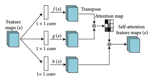
Assign a feature map , the input for the NILM task consists of L time steps and C channels. First, the input is converted into two feature spaces f(x) = Wfx and g(x) = Wgx for computing the attention map.
3.1.3. Two Subnetworks
The structure of the two subnetworks, consisting of the subnetwork of regression and the subnetwork of classification as proposed in [31], is visualized in Figure 4.
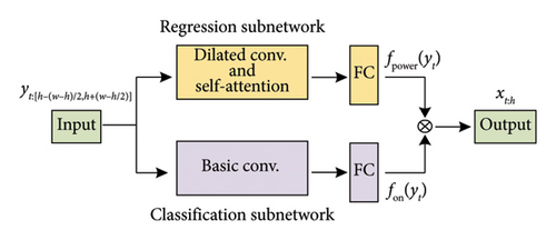
The subnetwork of regression and classification are designed to make predictions or provide estimations for the power consumption and the operational status of the target appliance (whether it is on/off), respectively. The aggregate power consumption with the window length w serves as the input, and the midpoint, denoted by k, of the target appliance’s window with a specific length w is the output predicted by the system.
In this context, ⊙ refers to element-wise multiplication.
3.2. Dual-Subnetwork Model Based on Stacked Dilated Convolutions and Self-Attention Mechanism
In this article, we use the two subnetworks structures and combine them with seq2point learning. We propose a new regression subnetwork that includes the dilated convolution and the self-attention mechanism.
The structure that we proposed is illustrated in Figure 5. We added a stacked dilated convolutional layer composed of three dilated convolutions to the fourth layer of the regression network. The dilated convolutions used in stacked dilated convolution layers have the same filter size and number of convolution filters, with increasing dilation rates of 1, 2, and 3. Subsequently, the stacked dilated convolution layer produces its output by aggregating the feature outputs of the three dilated convolutions into a single tensor based on the channel dimension.
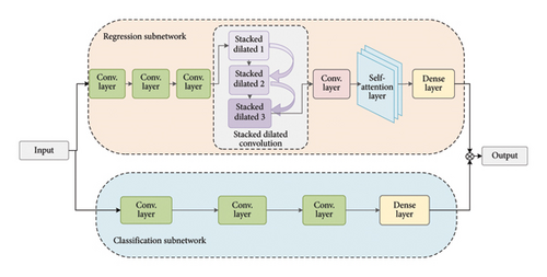
Before sending the multiscale contextual information into the self-attention layer, the convolutional layer with a filter size of one is used to reduce the dimension of multiscale contextual information. Otherwise, the quantity of parameters in the connected layer will undergo a substantial increase. The dimension-reducing convolutional layer has 32 filters, thus for the self-attention layer. After calculating the correlation of the global contextual information through the self-attention layer, the important features will get more attention. The midpoint of the target appliance sequence is the output from the regression subnetwork.
In classification subnetwork structure, the convolution filter sizes are adjusted to 10, 8, 6, 3, 3, 3, and 3, while keeping all other parameters unchanged.
The equations above demonstrate that the regression subnetwork is active only when the classification subnetwork identifies the target appliance’s state as “on”. This is because when the classification subnetwork classifies the state as “off”, the gradient of the regression subnetwork is zero. Therefore, the regression subnetwork can get better performance because it is not easily affected by interference from other appliances.
4. Experiment and Results
This section describes the overall model architecture used in this study, details the dataset employed, and outlines the performance metrics applied. Subsequently, experimental results are analyzed and discussed.
4.1. Experiment Settings
4.1.1. Model Parameters and Structure
Our research experiments were conducted using Python 3.6.7 and TensorFlow 2.3. We utilized the Adam optimizer with an initial learning rate of 0.0001 and a batch size of 16.
The structure and output modes of the regression subnetworks of the proposed twin network are illustrated in Figure 6.

In Figure 6, we provide an explanation of the primary regression subnetwork. Initially, the input undergoes three layers of convolutional processing before entering the dilated convolutional layer. In these three dilated convolutional layers, the number of filters and the kernel size remain constant, while the receptive field is progressively enlarged by increasing the dilation rate, thus capturing a broader context. Subsequently, the outputs of the dilated convolutions are combined to form a feature tensor. Following this, the feature tensor is passed through a self-attention layer to compute the relevance of global context information, enhancing useful features while suppressing irrelevant ones. Output of the regression subnetwork is multiplied by the output of the classification subnetwork to obtain the final result. It is worth noting that the regression unit is only activated when the classification subnetwork identifies the state of the target device as “on”. Hence, the proposed model possesses the advantage of being less susceptible to interference.
The parameter settings are shown in Table 1. In the convolutional layers and the fully connected layers, the ReLU activation function is used, which helps the network learn nonlinear relationships while mitigating the vanishing gradient problem. In the output layer of the regression network, a linear activation function (Linear) is used, which avoids applying any nonlinear transformation, making it more suitable for continuous value outputs. In the output layer of the classification network, the Sigmoid activation function is employed, which compresses real numbers into the (0, 1) interval and is commonly used in binary classification networks.
| Network type | Number of filters | Convolution kernel size | Stride | Dilation rate | Padding | Initialization | Activation function |
|---|---|---|---|---|---|---|---|
| Standard convolution | 30 | 10 | 1 | — | Same | he_normal | ReLU |
| Standard convolution | 30 | 8 | 1 | — | Same | he_normal | ReLU |
| Standard convolution | 40 | 6 | 1 | — | Same | he_normal | ReLU |
| Stacked dilated convolution 1 | 50 | 3 | 1 | 1 | Same | he_normal | ReLU |
| Stacked dilated convolution 2 | 50 | 3 | 1 | 2 | Same | he_normal | ReLU |
| Stacked dilated convolution 3 | 50 | 3 | 1 | 3 | Same | he_normal | ReLU |
| Conv_ave | 32 | 1 | 1 | — | Same | he_normal | ReLU |
| Dense | 1024 | — | — | — | — | he_normal | ReLU |
| Regression subnetwork | Length | — | — | — | — | he_normal | Linear |
| Output layer | Output | ||||||
| Classification subnetwork | Length | — | — | — | — | he_normal | Sigmoid |
| Output layer | Output | ||||||
The training period for the proposed model in this paper is set to 150 epochs, during which the model will undergo 150 complete iterations over the entire training dataset. Within each epoch, the training dataset is divided into multiple batches, specified as 16. The model sequentially reads data batch by batch, performs forward propagation, computes loss, conducts backward propagation, and updates parameters until all data in the training dataset have been used for training.
4.1.2. Dataset
The high-frequency data relies on the equipment with a higher sampling frequency, which is unsuitable for residential users. Hence, our primary focus is on the low-frequency data. The experiments are conducted on the dataset UK-DALE [42].
The UK-DALE low-frequency dataset, released in 2015, records the whole-house active power consumption data of five UK households at a frequency of 1/6 Hz from November 2012 to January 2015, along with active power consumption data for over a dozen types of appliances. The UK-DALE dataset is provided in a standard CSV format, which makes it easy to handle and analyze. It includes timestamps and the power consumption of various appliances. Additionally, the dataset provides appliance state labels, which record the on/off states of each appliance at each time point, such as when appliances like WM and refrigerators (FD) are turned on or off.
House1, House2, and House5 also record the total active power consumption of the households at 1 Hz and voltage and current data at 16 kHz. FD, kettles (KE), dishwashers (DW), and WM were selected as they are commonly studied in various research contexts. These appliances exhibit multiple power consumption patterns, ranging from binary-state appliances such as FD and KE to multistate appliances such as DW and WM. Therefore, these devices are often considered typical examples. The selected appliances comprehensively validate the disaggregation capability of the proposed model.
Following previous studies [30, 31], for training, we utilize the data from House1 and House5, reserving the data from House2 for testing. For data normalization, the mains data and the appliance data are divided by their respective standard deviations. Similar to the previous study [30], the appliance’s parameters and window lengths are detailed in Table 2.
| Appliance | Windows length | Mean power (W) | Standard deviation | Power threshold (W) |
|---|---|---|---|---|
| FD | 599 | 200 | 400 | 15 |
| KE | 599 | 700 | 1000 | 200 |
| DW | 599 | 700 | 1000 | 15 |
| WM | 599 | 400 | 700 | 15 |
The selection of appliance threshold is primarily determined based on the power consumption states of the appliances. For appliances with simple states, such as KE, the threshold is set to 200. Appliances with lower power consumption, such as FD, and those with multiple operational states, such as WM and DW, have their thresholds set to 15.
The input to the model consists of the real-time total active power sequence composed of the running power of all appliances in the household, rather than a simple combination of active power sequences for the four aforementioned appliances. The input data format of the proposed model is a time series, containing the power consumption of each appliance at every time point. In other words, each row corresponds to a time point, and each column corresponds to the power consumption value of an appliance. This format of input data effectively conveys the temporal correlations and interactions among appliances, enabling the model to learn better.
4.1.3. Evaluation Metrics
4.2. Results
4.2.1. Dual-Network Architecture Optimization
In this study, a dual-network model was employed to enhance the accuracy of load disaggregation, proving to be less susceptible to interference from other devices compared to the single regression network model. Figure 7 illustrates the comparison between the outputs of a single regression network and the dual-network model.
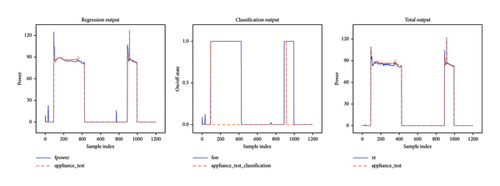
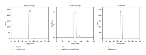
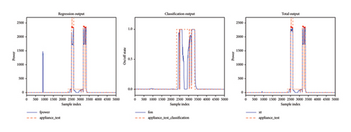
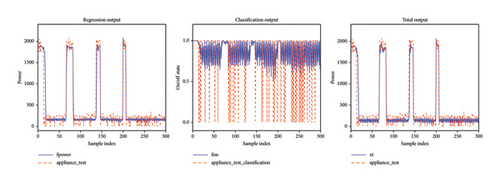
From Figure 7, it is evident that for all appliances, the total output obtained after processing through the classification subnetwork and regression subnetwork achieves better disaggregation accuracy and lower error compared to the single regression network. In Figure 7(a), the total output for the fridge is closer to the actual energy consumption profile and shows more stable fluctuations. During peak energy consumption, the dual-network model can more accurately predict and track these peaks. This demonstrates that the dual-network model is more stable and effective in capturing actual energy consumption fluctuations, providing more reliable energy consumption predictions. In Figure 7(b), the dual-network model precisely captures the energy consumption peaks of the KE, aligning very well with the actual energy peaks. This displays the high precision of the dual-network model in predicting short-term, high-peak energy events. In Figure 7(c), the total output better matches the actual energy consumption data, with fewer deviations, especially at the peaks of energy consumption. Figure 7(d) shows that under frequent switching conditions of the WM, the output of the dual-network model demonstrates higher accuracy and more accurately matches the actual electricity usage during operation. Therefore, the dual-network model proposed in this paper has a better disaggregation effect.
4.2.2. Running Time
Considering that our proposed model is a combination of different algorithms, there might be a risk of longer runtime. Hence, we conducted systematic performance testing in experiments.
To ensure fair comparison of algorithm performance, model parameter size, and training duration, we used the same optimizer and learning rate for the comparative algorithms used in this study, along with other relevant settings kept identical. While our proposed model improves performance, it also maintains a parameter count in the order of tens of thousands, providing a certain advantage compared to seq2point and RNN models. The comparison results are shown in Table 3.
| Model name | Training parameters | Time (s/epoch) | Decomposition time (s) |
|---|---|---|---|
| RNN | 1,264,977 | 797 | 0.0749 |
| GRU | 454,513 | 117 | 0.0458 |
| Seq2point | 11,713,049 | 90 | 0.0095 |
| Proposed model | 232,212 | 252 | 0.0450 |
The proposed model requires 252 s for training a single epoch, which is acceptable in offline training environments for practical engineering applications. The processing time for 1 hour of electricity data for all four models is less than 1 s, meeting the real-time requirements in engineering applications. This ensures that our model has acceptable operational efficiency in practical applications, achieving significant improvements in evaluation metrics while ensuring accurate results within a reasonable timeframe.
4.2.3. Experimental Verification
We chose three different NILM algorithms, which are RNN [28], GRU [29], and seq2point [30]. RNN models are adept at capturing dependencies in time series data, while GRU models effectively capture both short-term and long-term dependencies, resulting in better performance and reduced computational complexity. Seq2point is efficient in handling load disaggregation tasks. We used these three algorithms to compare with our proposed method.
To gauge or assess the switch status of appliances, we use the classification metrics F1 score. In this experiment, the true positive (TP) rate reflects the device’s correct identification when in the “on” state. The false positive (FP) rate indicates instances where the device is incorrectly classified as “on” when it is actually off. The false negative (FN) rate represents cases where the device is erroneously identified as “off” when it is actually on. Precision (P) denotes the proportion of TP among all identified “on” states, while recall (R) indicates the proportion of times the device being “on” is correctly identified as such.
Table 4 presents the performance comparison between proposed model and the prior work, with the best performance for each appliance highlighted in bold. The results show that proposed model achieved lower MAE and SAEσ across all appliances, outperforming other NILM algorithms. Compared to the RNN and GRU algorithms, the proposed model’s performance is significantly superior, approximately twice as advantageous in the overall evaluation metrics. Specifically, compared to the seq2point model, the proposed model improves the average MAE, SAEσ, and F1 score by 13.85%, 21.27%, and 26.15%, respectively. Therefore, the algorithm proposed in this paper provides an effective and practical solution to the NILM problem, making it suitable for large-scale real-world engineering applications.
| Model | Metric | FD | KT | DW | WM | Average |
|---|---|---|---|---|---|---|
| RNN | MAE | 27.89 | 22.24 | 42.14 | 20.17 | 28.11 |
| SAE | 17.40 | 16.55 | 41.81 | 17.78 | 23.39 | |
| F1 | 0.70 | 0.49 | 0.40 | 0.13 | 0.43 | |
| GRU | MAE | 24.36 | 16.93 | 34.88 | 19.18 | 23.84 |
| SAE | 14.87 | 13.39 | 33.47 | 17.95 | 19.92 | |
| F1 | 0.80 | 0.49 | 0.57 | 0.23 | 0.52 | |
| Seq2point | MAE | 20.06 | 9.35 | 27.15 | 12.75 | 17.33 |
| SAE | 11.77 | 5.34 | 22.84 | 9.35 | 12.32 | |
| F1 | 0.84 | 0.85 | 0.62 | 0.30 | 0.65 | |
| Proposed model | MAE | 19.23 | 6.64 | 23.15 | 10.68 | 14.93 |
| SAE | 10.85 | 4.48 | 16.04 | 7.42 | 9.70 | |
| F1 | 0.85 | 0.92 | 0.75 | 0.76 | 0.82 | |
- Note: The bold values present the performance comparison between proposed model and the prior work, with the best performance for each appliance highlighted in bold.
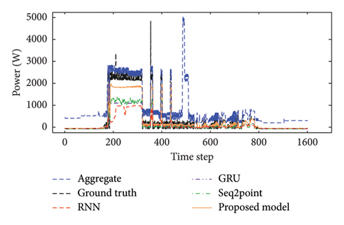
Figure 8 presents a comparison among the four methods: RNN, GRU, seq2point, and the proposed model. This comparison is conducted across appliances with different electrical characteristics. Figures 8(a) and 8(b) represent typical single-state appliances, while Figures 8(c) and 8(d) represent typical multistate appliances. It is evident that the proposed model consistently achieves the most optimal and precise load disaggregation results across all appliances.
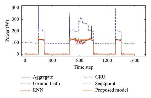
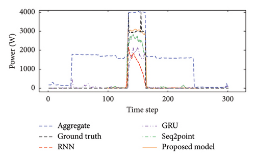
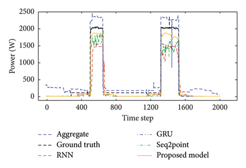
In Figure 8(a), it is observed that while all four models are relatively effective in detecting and disaggregating the operational power of the fridge, there are noticeable differences in their disaggregation performances. The comparison models show varying degrees of fluctuation in their disaggregation values. The proposed model exhibits the best disaggregation performance; however, it still falls short of accurately capturing the peak power generated during the fridge’s startup. Figure 8(b) shows that when multiple devices are running simultaneously, GRU and seq2point are more susceptible to interference, leading to erroneous “on” states. In contrast, RNN and the proposed model demonstrate better anti-interference capabilities. Additionally, compared to RNN, the proposed model’s disaggregation results are closer to the actual operating values of the appliances, indicating superior disaggregation capability.
For multistate appliances such as DW and WM, Figure 8(c) indicates that RNN and GRU have relatively smooth curves, demonstrating good stability and reduced susceptibility to short-term noise. The gated mechanism in GRU more effectively captures the long-term dependencies in sequence data. However, the prediction accuracy of RNN and GRU is not high. Both seq2point and the proposed model are closer to the true values of the appliances. Nonetheless, seq2point’s disaggregation results show instability, being highly sensitive to noise and interference in the data, which limits its load disaggregation capabilities. In contrast, the proposed model exhibits less fluctuation and is closer to the appliance’s actual operating state, outperforming the other three load disaggregation methods. Figure 8(d) visually highlights the advantages of the proposed model. Compared to RNN, GRU, and seq2point, the proposed model has a higher capability of approaching the true values, demonstrating superior recognition ability and anti-interference performance. Moreover, the probability of misjudging the switch states is significantly lower than that of the other three methods.
The on/off states of multistate appliances are visualized in Figure 8, and the on/off state performance is shown in Table 5. It is clear that the proposed model has higher precision and F1 score than the seq2point model.
| Model | Metric | Washing machine | Dishwasher |
|---|---|---|---|
| Seq2point | Precision | 0.18 | 0.45 |
| F1 score | 0.30 | 0.62 | |
| Proposed model | Precision | 0.88 | 0.64 |
| F1 score | 0.76 | 0.75 | |
- Note: The bold values present the performance comparison between proposed model and the prior work, with the best performance for each appliance highlighted in bold.
Figure 9(a) illustrates the on/off states of the DW. It can be observed that both models accurately identify the states of appliances, particularly multistate appliances like DW. However, the seq2point model is more susceptible to interference from other devices, leading to multiple misjudgments before and after switching. The proposed model exhibits fewer misjudgments compared to the seq2point model and is noticeably less affected by other devices’ interference. Figure 9(b) presents the on/off states of the WM. It shows that when the WM is not in operation, the seq2point model frequently misjudges the state as “on.” This is because the seq2point model struggles to learn the complex characteristics of multistate appliances like WM, and it is more prone to interference from other devices, resulting in more frequent misjudgments. Our proposed model, on the other hand, can learn the intricate features of these multistate appliances. This is primarily attributed to the incorporation of stacked dilated convolution and self-attention mechanisms in our model, which enable the extraction of higher-level features from raw data. The self-attention mechanism helps the model capture important contextual information globally, while the stacked dilated convolution effectively expands the model’s receptive field. Consequently, our model achieves more accurate load disaggregation results.

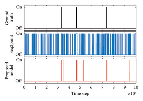
Figure 10 shows feature maps of multiple scales for the DW, with a total of 599 (window length) time steps. Specifically, each feature map has 50 channels (vertical axis) and 599 time steps (horizontal axis).
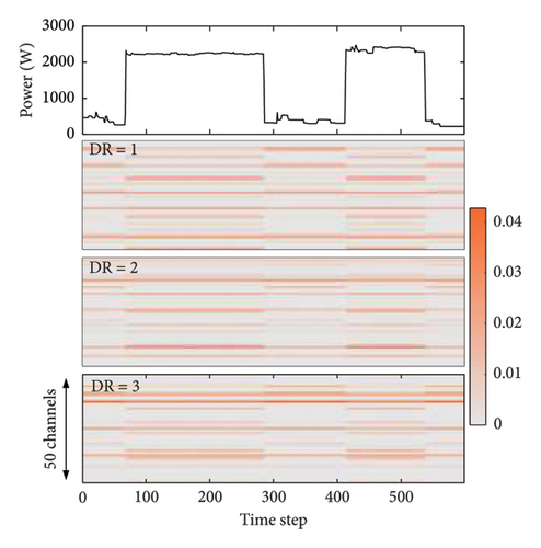
It is seen that when the dilation rate of the dilated convolution varies, the obtained feature maps also have significant differences. Although the three feature maps are different, they can all respond to the upward and downward transitions of the DW, and each channel has a different degree of attention to the features of the DW. Multiscale contextual information can be acquired by linking feature maps with various dilation rates.
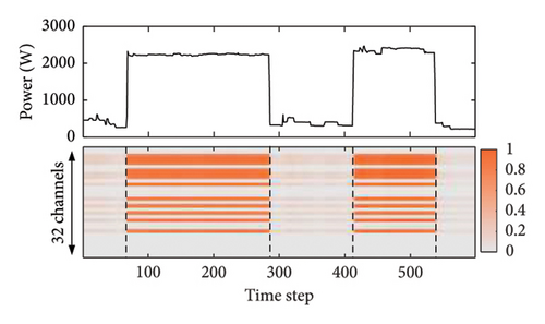
Figure 11 depicts the feature map generated by the attention layer for the DW. It is evident that the feature map after the self-attention layer differs significantly from the contextual feature map shown in Figure 10. Unlike Figure 10, the values of the feature map in the self-attention layer are closer to each other under the same operating state of the DW. Therefore, it demonstrates that the self-attention mechanism has the ability to redistribute attention across relevant features.
5. Conclusion
In this paper, we first proposed a seq2point regression subnetwork model based on stacked dilated convolution and self-attention mechanism, and then combined the regression subnetwork with the classification subnetwork to form a two-subnetwork model. Experimental results demonstrate a significant enhancement in the performance of the proposed model for the NILM task, showing robust generalization capabilities as observed during training and testing across various appliance families.
However, for appliances with multiple states such as dishwashers and WM, the recognition accuracy of the model still falls below 80%. While the proposed model accurately captures the operation of various appliances, it struggles to precisely capture peak values during refrigerator startup. Although it performs better in disaggregating multistate appliances compared to previous models and avoids misjudging switch states, there remains a discrepancy from the Ground Truth. Overcoming these challenges will be a key focus of our future work. We plan to enhance the recognition accuracy and generalization ability for multistate appliances by optimizing additional methods in conjunction with the proposed model. Additionally, we aim to explore the transfer learning capability of our model. We plan to collaborate with companies that have extensive data on household appliance usage by their customers (ensuring user information confidentiality), in order to broaden the scope of our proposed model.
Currently, there exists a technology known as BTM systems, involving integrated energy storage systems, where residential households may have photovoltaic (PV), battery energy storage systems (BESS), and electric vehicle (EV) charging infrastructure on their premises. Therefore, the NILM process could be more challenging, making disaggregation issues harder to resolve. In the next phase, we intend to consider households with energy storage systems, studying related load characteristics and more.
Disclosure
This manuscript has been presented as a preprint [43].
Conflicts of Interest
The authors declare no conflicts of interest.
Funding
This work was supported by the National Natural Science Foundation of China (51977127), the Science and Technology Commission of Shanghai Municipality (19020500800), and the “Shuguang Program” (20SG52) funded by the Shanghai Education Development Foundation and Shanghai Municipal Education Commission.
Acknowledgments
The authors would like to thank the funding agencies and organizations that supported this research, as well as colleagues who provided valuable discussions and technical support.
Open Research
Data Availability Statement
The datasets used and analyzed during the current study are publicly available. Specifically, the UK-DALE dataset used in this study is accessible at [https://jack-kelly.com/data/].


