Parametric Analysis and Optimization of a Dual-Fuel-Fired Boiler for Power Generation Using the Taguchi Design Approach
Abstract
Increased energy supply reliability, environmental sustainability, more competitive businesses, and improved standard of living are all made possible by more efficient energy conversion processes. In view of this, the present study aims at analysis and optimization of the operational parameters of a dual-fuel-fired boiler using Taguchi design method to enhance boiler thermal efficiency and throughput for sustainable power generation. The L27 orthogonal array (OA) was employed with 27 experimental runs to assess the influence of the four identified design parameters: economizer outlet water temperature (EOWT), total airflow (TAF), gas air heater outlet temperature (GAHOT), and feed water temperature (FWT) on the boiler main steam flow (BMSF). Box–Behnken factorial design from Minitab 18 was used to analyze the effects of the design factors and runs on the response parameter. Results of the study reveal that the quadratic regression model developed with the Taguchi design predicted the BMSF at 95.5% confidence level. The optimal signal-to-noise (S/N) ratio of 56.57 and maximum BMSE of 674 T/h were achieved at the optimal design parameters of 257°C of EOWT, 64% of TAF, 237°C of GAHOT and FWT of 210°C at the boiler feed drum. The adequacy and degree of fitness of the quadratic models developed were determined using the coefficient of determination (R2), adjusted and predicted R2, and adequate precision. The coefficient of determination R2 values for the BMSF model and S/N ratio model are 0.9995 and 0.9990, respectively. The R2 values show that the developed models have a good fit and ability to predict BMSF and S/N ratio accurately. In addition, adjusted R2 (BMSF model: 0.9990; S/N ratio model: 0.9981) and predicted R2 (BMSF model: 0.9956; S/N ratio: 0.9955) values are in reasonable agreement as their difference is less than 0.2. Conclusively, this study shows that the most influential factor on BMSF is the EOWT with a percentage contributing ratio of 38%; this is followed by FWT with 36%. From the prediction analysis and with the optimized factors, the efficiency of the existing steam turbine power plant of 33% could be increased to 55%.
1. Introduction
The need for electricity has been steadily increasing in recent decades, necessitating the development of more efficient and environmentally friendly power-producing methods [1]. As a result, renewable energy sources are being examined as potential contenders for reducing carbon footprints and fulfilling global environmental goals such as the Paris Agreement and net-zero by 2050 [2, 3]. Renewable energy technologies, on the other hand, remain far from being deemed sustainable and reliable energy sources to meet global energy demands [4]. Furthermore, several developing and impoverished countries’ energy systems are significantly reliant on fossil fuel-based energy systems [5]. As a result, it is critical to develop techniques for reducing fossil fuel consumption (FC). As a key source of sustainable electricity, it is critical to concentrate on how to improve the performance and reliability of conventional thermal power plants, particularly steam power plants, in order to make the most efficient and effective use of finite fossil fuel resources [6].
A shift to extremely efficient and environmentally safe fossil fuel-based electricity-generating technology is necessary for the power industry to operate sustainably. Because of their high efficiency and ability to produce enormous amounts of electric energy, steam turbine power plants are used extensively throughout the world. The versatility of this kind of power unit to run on many fuels, its extended lifespan, and its broad range of power production are further factors contributing to its widespread use [7]. To accurately monitor a steam power plant’s operation, all of its major components should be examined for efficiency and effectiveness. Enhancing the efficiency of the steam power plant is therefore a crucial objective. Not only will the primary resource be preserved, but it will also mitigate harmful atmospheric emissions such as nitrogen oxides and carbon dioxide. Due to the implications of improved thermodynamic cycle performance for net incremental power output and investment cost savings, these improvements have also gained importance in the real global sustainability context for the efficient production of steam thermal power plants [8].
The soaring demand for energy necessitates optimizing thermal power plant operation and enhancing the performance of power plant equipment [9]. Because of this, studies of thermal power generation systems are of scientific interest and also essential for the efficient utilization of limited available energy resources. Several studies on component-based energy and exergy evaluation of steam thermal power plants have been performed and reported [10–13, 14, 15]. From the outcome of the previous research, boilers were identified as the main contributors to exergy destruction owing to their associated high irreversibility. That is, the boiler has high exergy improvement potential compared to other components of the steam power plant.
The backbone of a steam power plant is the boiler. It is unquestionably one of the most crucial components of industrial energy systems, as they convert fuel energy into heat needed for technological operations like electricity generation [16]. Boiler in thermal power plant plays an important role in generation of power. An effective control of the temperature and the pressure of boiler is necessary to enable safe power generation. For regulating the power generation, control of main steam from the boiler unit plays a major role [17, 18]. Subcritical boilers, supercritical boilers, and heat recovery steam generator (HRSG) are types of boilers commonly used to produce high-capacity steam. Many minor components make up an industrial steam boiler. If one of these components fails, the steam boiler will also fail, posing a significant issue for engineers in the electric power industry. According to studies, the steam boiler as one of the most important components in a steam power plant its performance assessment is essential [19]. The evaluation of such a component from a thermodynamic and reliability standpoint is critical for sustainable power plant [14, 20].
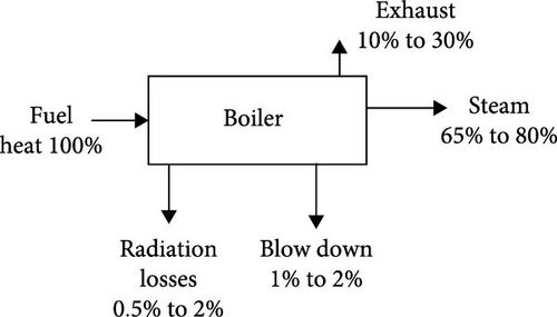
Because steam has a two-fold higher heat transfer coefficient than water, it is the primary input for several industries, whether they use it directly or indirectly. As a result, it may be effectively used in power generation plants to generate energy [21, 22]. Energy is consumed, conserved, and dissipated in steam boilers when engaged in producing steam for different end uses by combustion of fuel [23, 24]. In view of the importance of the steam boiler system in a steam power plant, experts are particularly interested in evaluating its performance and optimization. Evaluation of steam generation systems is essential in industries for effective energy usage [15]. Identifying the locations where energy waste is most likely to happen is essential to optimize the performance of a boiler plant. Because not all of the heat generated by burning fuel can be transferred to steam or water in the boiler, a considerable amount of energy is lost through flue gases. Research has shown that as the temperature of the flue gas leaving a boiler typically ranges from 150 to 250°C, about 10%–30% of the heat energy is lost through it [25, 26]. Figure 1 depicts a boiler’s typical heat balance. Since the majority of the boiler’s heat losses appear as heat in the flue gas, recovering this heat has the potential to save a significant amount of energy. This suggests that by reducing its losses, a boiler can save a significant amount of energy [28].
The increase in energy production cost is associated with inadequate production and distribution of heat energy in the boiler. To address this issue effectively, it is essential to evaluate the boiler system and identify areas for improvement. Because boiler efficiency plays a major role in both generating more energy and reducing production costs, it is imperative to analyze it. According to Talib et al. [29], boiler assessment analysis and accurate modeling are crucial for maximizing power plant performance for sustainable operation.
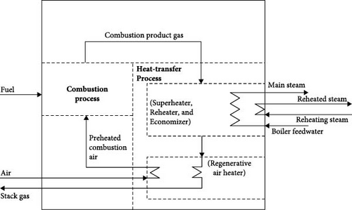
Effective steam energy production, for example, can result in lower operating costs, more productivity, and less energy consumption in a steam power plant [30]. It is necessary to pay attention to a number of operating conditions in order to achieve optimal steam energy output. Ensuring proper regulation of a boiler’s operational parameters is crucial, given the significant risks of explosion associated with high working pressures and temperatures [31, 32]. Several process parameters are monitored and regulated purposely to enhance the smooth operation and performance of the boiler. Parameters that governed the performance of a boiler are grouped into those that decide boiler heat input and heat output. Essentially, the parameters that decide boiler heat input are fuel to be fired, the calorific value of fuel, total airflow (TAF), feedwater quantity, feed water temperature (FWT), economizer outlet water temperature (EOWT), gas air heater outlet temperature (GAHOT), steam pressure and temperature, the temperature of the attemperator, etc. [33] While those that decide boiler heat output are; main steam flow, main steam temperature, main steam pressure, etc. [34]. This indicates that the boiler is a multi-input, multi-output, and interrelated complex control component (Figure 2). These operating parameters greatly influence key performance indicators such as efficiency and FC. Moreover, these key factors allow the boiler unit to produce high-quality steam, which is necessary to drive the steam turbine in a steam power plant for sustainable power generation [29, 35]. In seeking to achieve this, process parameters must be examined due to their close relation to boiler efficiency and FC, and their importance to the entire steam generation activity [36, 37].
Steam production in boilers is highly irreversible, driving the rising concern for the correct operation of industrial boilers. Researchers have investigated different approaches to enhance steam generation. and to improve the energy performance of boilers using direct and indirect approaches or based on thermodynamic models or statistical tools in correlating input parameters to output parameters. Cheridi et al. [38] investigated the overall behavior of a steam boiler using RELAP5/MOD3.2 system code at three different operating loads. Results of the study revealed that RELAP5 system code results match significantly with the experimental data of the steam boiler. In their study, Zhu et al. [39] proposed the combination of the long short-term memory (LSTM)-based dynamic model and the model predictive control architecture to inhibit the steam temperature fluctuations of a 1000-MW double-reheat coal-fired boiler. The suggested controller performs exceptionally well in regulating steam temperature, and the authors claim that the LSTM model may be used to capture the time delay, multivariable coupling, and nonlinear dynamics of the steam temperatures. By adjusting the operating parameters, Li et al. [40] assessed and optimized the pressure drop of the main steam pipe and the reheat steam pipe of a 1000 MW secondary reheat unit. They also explored the operational costs. By selecting a bend pipe and optimizing the pipe parameters, the optimal pipe specifications were achieved. Akerekan and Oyim [34] evaluated the boiler efficiency of a 220 MW steam power plant using the direct method. The study employed the input–output method based on ASME PTC 4.1 standard to determine the boiler efficiency. Results of the study revealed that the instantaneous data on boiler thermal efficiency can determine the condition of boiler operation, heat generation, and heat loss. In order to determine the quantity of fuel utilized by the boiler, Okwabi et al. [35] developed predictive models of feedwater temperature. The study’s findings showed that, at a 95% confidence level, the Autoregressive Moving Average model, ARMA (1,1), was able to forecast the feedwater temperature with an accuracy of ±3.967. The study found that the amount of fuel utilized by the steam boiler and the temperature of the feedwater have a negative linear relationship.
Cheridi et al. [38] presented the modeling and simulation of a water-tube steam boiler with natural circulation. Using the RELAP5/MOD3.2 system code, the study examined the general behavior of a steam boiler at three distinct operating loads. The generated model was shown to be appropriate for transient simulation, and the authors report that it was applied to the reconstruction of three steady-state tests to evaluate the safety aspects of the steam boiler during operation. The results of a pulverized coal-fired steam boiler examined under various operating conditions were presented by Madejsk and Zymełka [41]. To simulate how the boiler would operate with partial boiler loads, a thermodynamic model was developed for the study. Moreover, the indirect method and the computation of individual boiler losses were used to determine the energy efficiency of the boiler. A mathematical model to calculate the amount of saturated steam produced in maritime water tube boilers and smoke tube boilers was presented by Tunski et al. [42]. The amount and temperature of exhaust gas, the surrounding air, the engine power load, and the boiler tube position were all taken into account in the mathematical model that was developed. The model’s universality, according to the authors, allows it to be used for numerical experiments as well as calculations for boilers that are currently in use. These experiments can be used to ascertain the amount of steam produced by all boiler types utilized in waste heat recovery systems in power marine systems. Taler et al. [43] presented a method to determine thermo-flow parameters for steam boilers. This method allows researchers to perform calculations of the boiler furnace chamber and heat flow rates absorbed by superheater stages. These parameters are significant for monitoring the performance of a steam power plant unit.
Studies on thermodynamic assessment and optimization of boilers’ performance parameters have been carried out. Egeonu et al. [44] assessed thermodynamic optimization of steam boiler parameters using a genetic algorithm. The result of the study revealed that applying the genetic algorithm in the thermodynamic optimization of the selected boiler, the percentage increase in the thermal efficiency was 4.76% and 3.89% in comparison with the existing values for the studied boiler at the Egbin thermal power plant for 2008 and 2009, respectively. Thermodynamic performance assessment and optimization from first and second laws have been carried out by several authors (Koochakinia et al. [20]; Jamali et al. [22]; Ohijeagbon et al. [23]; Molina et al. [26]; Nkoi et al. [32]). The uniform reports of the researchers show that the highest energy loss and exergy destruction occurred in the combustion chamber of the boiler.
Applications of statistical techniques such as Taguchi method and analysis of variance (ANOVA) for parametric assessment and optimization of boilers sparsely exist in literature. Using the Grey-Taguchi method, Talib et al. [29] assessed the performance of a coal-fired water tube boiler at a Pakistani cement company. In the study, the performance parameters—such as steam temperature, steam pressure, and specific steam flow rate—were optimized against FC and load using the Grey-Taguchi method. The study’s findings showed that the best-performing parameters satisfied the optimal requirements when they were observed at a load of 66% and an overall grey relational grade (OGRG) of 0.891. Morakinyo and Bamigboye [45] used the Taguchi design technique to optimize the operating parameters of a biomass fire-in-tube boiler in order to improve the boiler’s thermal efficiency and throughput. Chandrasekharan et al. [18] performed statistical modeling on the subcritical boiler systems, including the superheater, drum, and economizer. Analysis techniques, such as R2 analysis and ANOVA, were used to evaluate the effectiveness of the developed models. An analysis was conducted on the temperature’s reliance on several controlled variables. Orthogonal array (OA) L16 was used by Sathish et al. [46] to investigate steam generation using four process parameters and four levels. The chosen process parameters consisted of the temperature of feed water (°C), pressure of feedwater (bar), cold water supply (liters), and boiler drum pressure (bar). As the main target of the study was steam generation (in liters), hence, steam generation was selected as the process response. As most of the response values were within the desired range, the study’s findings showed that the experimental value of the steam generation was compared with the predicted value. Moreover, the maximum steam generation was achieved as 84.31 L which was recorded in the 15th run of the experiment.
To the best of the authors’ understanding, application of the Taguchi-based statistical technique combined with ANOVA for the optimal performance of boilers in thermal power plants is scanty in literature. More importantly, such analysis has not been carried out on the selected steam power plant in Nigeria. In this study, four key design factors (input parameters) namely, EOWT, TAF, GAHOT, and FWT are investigated with the aim to determine the optimal combination of the design variables that maximize the boiler main steam flow (BMSF) for sustainable power generation. Moreover, a quadratic regression model for predicting BMSF is to be developed. The operational parameters investigated in this study are scarcely considered in boiler performance assessment and optimization. Hence, this contributes to existing knowledge in the analysis and optimization of boilers in thermal power plants. The operational parameters considered in this study allow the boiler unit to produce high-quality steam, which is necessary to drive the steam turbine in a steam turbine power plant for power generation.
2. Materials and Methods
In this study, data were collected from a typical dual-fired steam power plant with 1320 MW capacity for over a period of 18 months. Then, the analysis was carried out using a statistical software package, MINITAB 18 and Excel software.
2.1. System Description
The heart of the power generation plant in Nigeria is the Egbin steam power plant, which is the focus of this study. Egbin is notably the largest generation power plant in West Africa with an installed capacity of 1320 MW. It was strategically located in a low land area in Ijede, Ikorodu, bounded by the Lagos lagoon, to aid heat exchange and energy dissipation. This power plant supplies about 15% of the total electricity consumption of the general populace, which makes it very key in the overall power mix [47]. Unfortunately, it has been operating far below the installed capacity due to several maintenance challenges, which are peculiar to a plant of this age and magnitude [48].
According to Egbin Design Manuals [49], the boiler, turbine, and generator (well-known as the B–T–G) system is the critical equipment necessary for the generation of energy in Egbin steam generation plants. All additional types of apparatus in the plant are termed auxiliaries, and they are required for the excellent running of the boiler compartment in the station. However, this study is focused on the boiler performance assessment and optimization.
2.2. Steam Generation Flow in Egbin Thermal Power Plant
The Egbin thermal power plant is a gas-fired plant with six 220 MW independent boiler turbine units. It can also run on high pour fuel oil, commonly called HPFO. The steam boiler was designed to deliver steam at temperature ranges from 541 to 600°C and pressure of 12,500 kPa to the turbine. The boiler is employed to reheat steam discharged from the high-pressure (HP) turbine after a generating cycle, using the combustion of heavy fuel oil or natural gas as a source of energy. Table 1 shows the detailed design parameters of the boiler at the Egbin power plant. The boiler is of the Radiant type, natural circulation with single reheat and dual fuel firing. It was manufactured in the year 1985 by Babcock-Hitachi Company.
| Boiler parameter | Design value |
|---|---|
| Superheater outlet steam flow | 700T/h (MCR) |
| Superheater outlet steam pressure | 12,500 KPa |
| Superheater outlet steam temperature | 541°C |
| Reheater outlet steam temperature | 541°C |
| Feedwater temperature (gas firing) | 204°C |
| Fuel flow rate | 43-45T/H (MCR) |
At the Egbin power plant, during ambient cold starting, feed water from the demined storage tank is fed via the boiler filling pumps to the boiler drum where a separator/cyclone separates the water from the steam (Figure 3) [51]. The steam flows to the primary superheater where the first stage of superheat is absorbed by convection. The steam then flows to the secondary superheater. Between these two superheaters is a spray attemperator that controls the heat of the steam entering the secondary superheater at higher loads from 110 MW. Steam temperature here is 541°C and 12.5 MPa. From here, steam goes through the main steam pipe to impinge on the HP turbine blades at 538°C and a pressure of 12.5 MPa.
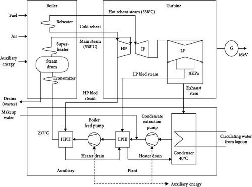
The cold reheat from the HP turbine enters back to the boiler and comes out a hot reheat at 541°C maximum continuous rating, which then impinges on the intermediate pressure (IP) turbine blades. From here, the steam via a cross-over pipe goes to impinge on the low-pressure (LP) turbine blades. The exhaust from the LP turbine at a pressure of 8 kPa goes to the condenser, where it is condensed into the Hot-well. The temperature of the condensate being 40°C. The condensate, at loads than 110 MW is pumped by the condensate extraction pump (CEP) to the deaerator via the LP Heaters (1–3). The LP heaters raise the temperature of the condensate to 134°C. But at higher loads (110 MW and above), the condensate booster pump (CBP) serves to boost the pressure of the condensate from the CEP. When necessary, the condensate is channeled via the condensate polishing plant (CPP) to free it of impurities. In the de-aerator, the feed water is doused with hydrazine to free the water from oxygen and temperature raised to 163°C after which boiler feed pumps (BFPs) pumps the feed water through the HP heaters (5 and 6) back to the boiler drum via the economizer for the cycle to continue. The temperature of the feed water entering the economizer is 237°C at a pressure of 13.7 MPa.
2.3. Mathematical Modeling of the BMSF Using Taguchi Method
Taguchi’s L9 robust design technique is a dynamic statistical method employed to analyze experimental or theoretical data over some time. The method has a great ability to develop a predictive model for the optimal performance of an engineering system (the BMSF as considered in this study). The design of the experiment has a specific configuration of OAs, which involves the L4(23), L8(27), L9(34) … …..L64(421). These arrays significantly enhance the experimental analysis, reduce stress, idle time, lower the cost of operation, and also help to identify significant parameters involved during the services. Taguchi is used for high-quality system design, which uses the signal-to-noise (S/N) ratio to evaluate the factors performance and the error occurrence deviation of the desired response value. However, the S/N ratio is an analysis that depends on response investigation, and the various applications include the smaller, the better (SB) (minimize the response), the normal the better (NB) (target the response and you want to base the S/N ratio on means and standard deviations), and the higher, the better (HB) (maximize the response).
2.3.1. Selection of OA
This study used the Taguchi experimental design technique to analyze and optimize the performance of the BMSF at Egbin steam power plant, Nigeria. The design factors and response parameters considered in this study for optimization of the boiler performance and reliability are the EOWT (°C), TAF (%), GAHOT (°C), and FWT (°C). The output (or response) parameter is BMSF (T/h).
The utilized input data of these key relevant factors used to analyze the performance of the BMSF as obtained from the selected power plant are presented in Table 2.
| Operating parameters | Symbols | Level 1 | Level 2 | Level 3 |
|---|---|---|---|---|
| Economizer outlet water temperature (°C) | EOWT | 241 | 242 | 257 |
| Total airflow (%) | TAF | 40 | 53 | 64 |
| Gas air heater outlet air temperature (°C) | GAHOT | 221 | 237 | 248 |
| Feedwater temperature (°C) | FWT | 210 | 224 | 245 |
To conduct a successful Taguchi analysis, it is crucial to carefully choose a suitable OA. The selection of the OA is based on the total degree of freedom, which represents the sum of individual factors’ degrees of freedom. The degree of freedom for each factor is calculated as the difference between the number of levels of the factor and 1 [52].
The selected system has three components and four levels, giving it a DOF of 8. Conventionally, the OA concerning the Taguchi method should be larger than the total DOF value. Hence, L27 (34) was chosen as the Taguchi OA for this study. Taguchi L27 OA was used because it helps to obtain high optimal values to analyze the effects of the design factors on the response, and it also gives high optimization of the factors on the response. To obtain optimal operational conditions, the maximum BMSF in power plant is desired. Therefore, the higher, the better (HB) quality characteristics of BMSF are selected in the calculations. This simply means that the output (BMSF) must be larger or higher as possible.
Taguchi’s experimental design of OA L27 (34) was used to generate 27 experimental runs of independent operation parameters, which were numerically coded (1, 2, 3, and 4) to generate the matrix Table of nine OA L27 (34) shown in Table 3, while their empirical values are shown in Table 4. The experiments in this study are designed using a Taguchi L27 orthogonal standard array for the given input parameters. A statistical tool package, Minitab 18.0 was used to design the experiment to analyze and optimize the BMSF for the selected steam thermal power plant.
| S/N | EOWT | TAF | GAHOT | FWT |
|---|---|---|---|---|
| 1 | 1 | 1 | 1 | 1 |
| 2 | 1 | 2 | 2 | 2 |
| 3 | 1 | 3 | 3 | 3 |
| 4 | 2 | 1 | 2 | 3 |
| 5 | 2 | 2 | 3 | 1 |
| 6 | 2 | 3 | 1 | 2 |
| 7 | 3 | 1 | 3 | 2 |
| 8 | 3 | 2 | 1 | 3 |
| 9 | 3 | 3 | 2 | 1 |
| 10 | 2 | 1 | 1 | 3 |
| 11 | 2 | 2 | 2 | 1 |
| 12 | 2 | 3 | 3 | 2 |
| 13 | 3 | 1 | 2 | 1 |
| 14 | 3 | 2 | 1 | 3 |
| 15 | 3 | 3 | 3 | 2 |
| 16 | 1 | 1 | 1 | 3 |
| 17 | 1 | 2 | 3 | 2 |
| 18 | 1 | 3 | 2 | 1 |
| 19 | 2 | 1 | 3 | 1 |
| 20 | 2 | 2 | 2 | 3 |
| 21 | 2 | 3 | 1 | 2 |
| 22 | 3 | 1 | 2 | 3 |
| 23 | 3 | 2 | 3 | 1 |
| 24 | 3 | 3 | 1 | 2 |
| 25 | 1 | 1 | 2 | 1 |
| 26 | 1 | 2 | 1 | 3 |
| 27 | 1 | 3 | 3 | 2 |
| Level | EOWT | TAF | GAHOT | FWT |
|---|---|---|---|---|
| 1 | 532.7 | 584.3 | 585.0 | 534.0 |
| 2 | 618.7 | 568.3 | 620.0 | 619.0 |
| 3 | 672.7 | 671.3 | 619.0 | 671.0 |
| Delta | 140.0 | 103.0 | 35.0 | 137.0 |
| Rank | 1 | 3 | 4 | 2 |
2.3.2. Multiple Regression Model for Design of Experiment
2.4. ANOVA
2.5. Validation Procedure for the Experimental Model
3. Results and Discussion
3.1. Result of the L27 OA of the Taguchi Experimental Design
Results of the regression analysis of the design factors with the L27 OA of the Taguchi experimental design is presented in this section.
The S/N analysis was performed to optimize the BMSF in this study. Tables 4 and 5 show the response table for steam generation and response table for S/Ns, respectively. In this study, all the input design parameter values were transformed into mean and S/N ratio form for easy identification of the output, such as BMSF. From these Tables 4 and 5, EOWT has high influence on BMSF and it is followed by FWT, TAF, and GAHOT. Parameters influencing are concluded by rank value and delta value. Moreover, the level with the highest S/N is considered the optimum performance level. Hence, from Tables 4 and 5, third levels of EOWT, TAF, second level of GAHOT and third level of FWT are the optimum conditions for optimal performance of BMSF. Hence, the optimal combination of levels for the conditions of the highest response and highest S/N ratio are determined as (E3T3G2F3).
| Level | EOWT | TAF | GAHOT | FWT |
|---|---|---|---|---|
| 1 | 54.36 | 55.12 | 55.13 | 54.37 |
| 2 | 55.77 | 55.02 | 55.78 | 55.77 |
| 3 | 56.56 | 56.54 | 55.77 | 56.53 |
| Delta | 2.20 | 1.52 | 0.66 | 2.16 |
| Rank | 1 | 3 | 4 | 2 |
3.2. ANOVA of Response-Surface Method (RSM)-Based Model for BMSF and S/N Ratio Prediction
The actual and predicted values for BMSF and S/N ratio according to RSM are presented in Table 6. The second-order (quadratic) models obtained for BMSF and S/N ratio prediction are given in Equations (11) and (12), respectively. The negative terms in the equations depict antagonistic effects on BMSF and S/N ratio, while the positive terms imply synergic effect. The adequacy and degree of fitness of the quadratic models were determined using coefficient of determination (R2), adjusted and predicted R2, coefficient of variance % (CV%) and adequate precision. As shown in Table 7, R2 values for BMSF model and S/N ratio model are 0.9995 and 0.9990, respectively. The R2 values show that the developed models have good fit and ability to predict BMSF and S/N ratio accurately. In addition, adjusted R2 (BMSF model: 0.9990; S/N ratio model: 0.9981) and predicted R2 (BMSF model: 0.9956; S/N ratio: 0.9955) values are in reasonable agreement as their difference is less than 0.2. Regression model is appropriate and adequate if the disparity between adjusted R2 and predicted R2 is less than 0.2 [59]. Another fit statistic to test the precision of the developed model is CV. Low CV obtained (BMSF model: 0.3401; S/N ratio model: 0.0783) implies good data reliability, a high degree of precision and little variation between the predicted and actual values. Also, adequate precision measures the S/N ratio. A ratio greater than 4 is desirable. Adequate precision of 177.3065 for BMSF model and 140.2140 for S/N ratio model indicate an adequate signal. The developed models can be used to navigate the design space and adequate for precision.
| Run | EOWT (°C) | TAF (%) | GAHOT (°C) | FWT (°C) | Actual BMSF (T/h) | Pred BMSF (T/h) | Actual S/N ratio | Pred. S/N ratio |
|---|---|---|---|---|---|---|---|---|
| 1 | 241 | 64 | 248 | 245 | 670 | 669.08 | 56.52 | 56.53 |
| 2 | 242 | 40 | 237 | 245 | 670 | 670.92 | 56.52 | 56.49 |
| 3 | 241 | 40 | 221 | 210 | 412 | 411.61 | 52.29 | 52.26 |
| 4 | 242 | 53 | 248 | 210 | 516 | 513.43 | 54.25 | 54.25 |
| 5 | 257 | 64 | 237 | 210 | 674 | 673.47 | 56.57 | 56.58 |
| 6 | 257 | 53 | 221 | 245 | 673 | 674.17 | 56.56 | 56.56 |
| 7 | 257 | 40 | 248 | 224 | 671 | 671.77 | 56.53 | 56.53 |
| 8 | 242 | 64 | 221 | 224 | 670 | 669.29 | 56.52 | 56.52 |
| 9 | 241.773 | 42.969 | 237.034 | 228.291 | 567.795 | 567.18 | 54.784 | 54.93 |
| 10 | 241.945 | 49.224 | 227.767 | 225.958 | 609.065 | 608.69 | 55.444 | 55.43 |
| 11 | 242.884 | 42.541 | 234.293 | 227.447 | 654.065 | 653.85 | 56.126 | 56.09 |
| 12 | 256.364 | 41.787 | 225.385 | 224.982 | 571.774 | 570.92 | 54.726 | 54.72 |
| 13 | 241.015 | 57.351 | 242.743 | 221.517 | 503.42 | 510.00 | 54.224 | 54.21 |
| 14 | 254.535 | 40.304 | 227.509 | 212.955 | 632.908 | 633.55 | 55.514 | 55.52 |
| 15 | 243.679 | 48.937 | 226.454 | 212.165 | 653.301 | 653.15 | 55.955 | 55.98 |
| 16 | 256.975 | 52.372 | 227.279 | 228.675 | 626.627 | 626.65 | 55.817 | 55.80 |
| 17 | 241.28 | 50.536 | 234.048 | 222.075 | 525.716 | 524.07 | 54.336 | 54.31 |
| 18 | 256.203 | 43.325 | 224.546 | 237.005 | 657.377 | 656.51 | 56.034 | 56.05 |
| 19 | 241.697 | 55.357 | 244.923 | 236.026 | 651.678 | 650.84 | 56.285 | 56.28 |
| 20 | 256.544 | 46.51 | 222.974 | 217.412 | 526.564 | 526.79 | 54.136 | 54.13 |
| 21 | 241.959 | 50.832 | 224.236 | 234.071 | 667.743 | 668.71 | 56.305 | 56.31 |
| 22 | 256.811 | 49.285 | 235.474 | 222.315 | 646.009 | 646.06 | 56.049 | 56.05 |
| 23 | 241.406 | 54.413 | 231.524 | 225.928 | 579.775 | 578.40 | 55.125 | 55.12 |
| 24 | 256.792 | 56.688 | 229.497 | 214.023 | 603.357 | 603.68 | 55.501 | 55.50 |
| 25 | 256.756 | 42.547 | 228.665 | 231.188 | 604.79 | 603.62 | 55.308 | 55.31 |
| 26 | 242.984 | 47.624 | 221.119 | 210.531 | 596.294 | 596.57 | 55.045 | 55.07 |
| 27 | 244.638 | 40.228 | 230.982 | 210.098 | 655.57 | 656.01 | 55.931 | 55.91 |
| Source | Sum of squares | df | BMSF | F-value | p-Value | — |
|---|---|---|---|---|---|---|
| Mean square | ||||||
| Model | 1.238E + 05 | 14 | 8840.62 | 2013.69 | <0.0001 | Significant |
| A-EOWT | 31,783.28 | 1 | 31,783.28 | 7239.50 | <0.0001 | Significant |
| B-TAF | 21,176.62 | 1 | 21,176.62 | 4823.55 | <0.0001 | Significant |
| C-GAHOT | 7961.40 | 1 | 7961.40 | 1813.42 | <0.0001 | Significant |
| D-FWT | 51,671.89 | 1 | 51,671.89 | 11,769.67 | <0.0001 | Significant |
| AB | 955.88 | 1 | 955.88 | 217.73 | <0.0001 | Significant |
| AC | 14,920.01 | 1 | 14,920.01 | 3398.44 | <0.0001 | Significant |
| AD | 3.06 | 1 | 3.06 | 0.6961 | 0.4172 | Insignificant |
| BC | 37.14 | 1 | 37.14 | 8.46 | 0.0108 | Significant |
| BD | 2.52 | 1 | 2.52 | 0.5732 | 0.4607 | Insignificant |
| CD | 0.0267 | 1 | 0.0267 | 0.0061 | 0.9389 | Insignificant |
| A2 | 69,386.61 | 1 | 69,386.61 | 15,804.68 | <0.0001 | Significant |
| B2 | 1.11 | 1 | 1.11 | 0.2538 | 0.6218 | Insignificant |
| C2 | 0.7118 | 1 | 0.7118 | 0.1621 | 0.6929 | Insignificant |
| D2 | 0.9762 | 1 | 0.9762 | 0.2224 | 0.6440 | Insignificant |
| Residual | 65.85 | 15 | 4.39 | — | — | — |
| Cor. total | 1.238E + 05 | 29 | — | — | — | — |
| C.V. % | 0.3401 | — | — | — | — | — |
| R2 | 0.9995 | — | — | — | — | — |
| Adjusted R2 | 0.9990 | — | — | — | — | — |
| Predicted R2 | 0.9956 | — | — | — | — | — |
| Adeq precision | 177.3065 | — | — | — | — | — |
| S/N ratio | ||||||
| Model | 28.66 | 14 | 2.05 | 1080.96 | <0.0001 | Significant |
| A-EOWT | 6.60 | 1 | 6.60 | 3487.26 | <0.0001 | Significant |
| B-TAF | 5.53 | 1 | 5.53 | 2921.49 | <0.0001 | Significant |
| C-GAHOT | 2.29 | 1 | 2.29 | 1211.14 | <0.0001 | Significant |
| D-FWT | 11.80 | 1 | 11.80 | 6232.75 | <0.0001 | Significant |
| AB | 0.2456 | 1 | 0.2456 | 129.67 | <0.0001 | Significant |
| AC | 2.90 | 1 | 2.90 | 1530.92 | <0.0001 | Significant |
| AD | 0.0000 | 1 | 0.0000 | 0.0107 | 0.9191 | Insignificant |
| BC | 0.0222 | 1 | 0.0222 | 11.69 | 0.0038 | Significant |
| BD | 0.0005 | 1 | 0.0005 | 0.2863 | 0.6004 | Insignificant |
| CD | 5.894E−06 | 1 | 5.894E−06 | 0.0031 | 0.9563 | Insignificant |
| A2 | 13.76 | 1 | 13.76 | 7263.82 | <0.0001 | Significant |
| B2 | 0.0015 | 1 | 0.0015 | 0.7660 | 0.3953 | Insignificant |
| C2 | 9.105E−06 | 1 | 9.105E−06 | 0.0048 | 0.9456 | Insignificant |
| D2 | 0.0016 | 1 | 0.0016 | 0.8407 | 0.3737 | Insignificant |
| Residual | 0.0284 | 15 | 0.0019 | — | — | — |
| Cor total | 28.69 | 29 | — | — | — | — |
| C.V. % | 0.0783 | — | — | — | — | — |
| R2 | 0.9990 | — | — | — | — | — |
| Adjusted R2 | 0.9981 | — | — | — | — | — |
| Predicted R2 | 0.9955 | — | — | — | — | — |
| Adequate precision | 140.2140 | — | — | — | — | — |
- Note: p < 0.05: significant; p > 0.05: insignificant.
- Abbreviation: df, degree of freedom.
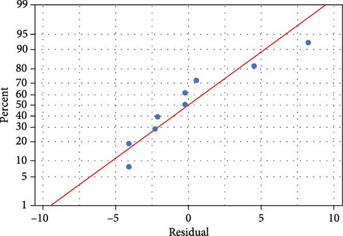
Figure 4 shows the normal probability plot for the BMSF. To analyze the normality of outcomes from experiments, normal probability plot is used. This plot shows the relationship between predicted response values and actual response values for the experimental layout designed for the study. When ANOVA is performed, it is mandatory to draw the normal probability plots for residual spectrum, which is situated near the mean line. From Figure 4, it is apparently seen that the residual values are near the mean line, that is, errors are not closely packed, but distributed normally. By means of regression analysis, the correlation between BMSF and the design factors in evaluating the performance of the boiler in the selected steam power plant can be obtained. The developed Taguchi model using regression Equation (4) for this study is presented in Equation (11). The predicted results obtained by Equation (11) are shown in Table 6 and the model coefficients is presented in Table 8. The coefficient of the factors is in multicollinearity by the VIF value of two (2) and above. This multicollinearity shows the effectiveness of the regression model in Equation (11) on the prediction accuracy of the response. Statistical analysis of the design parameters considered in this study shows that the mean and standard deviation values of EOWT, TAF, GAHOT, and FWT are 246.7°C and 7.76; 52.3% and 10.40; 235.3°C and 11.76 and 226.3°C and 15.26, respectively. The highest frequency levels of all the design parameters are noted as 1.0 for EOWT, 1.7 for TAF, 1.49 for GAHOT, and 1.15 for FWT.
| Term | Coef | SE coef | T-value | p-Value | VIF. |
|---|---|---|---|---|---|
| Constant | 538.07 | 7.37 | 72.97 | 0.009 | — |
| SNRA1 | 134.95 | 3.87 | 34.83 | 0.018 | 2.75 |
| EOWT | |||||
| 241 | −1.21 | 5.63 | −0.22 | 0.865 | 2.68 |
| 242 | −4.09 | 4.22 | −0.97 | 0.51 | 1.51 |
| TAF | |||||
| 40 | 2.69 | 4.73 | 0.57 | 0.671 | 1.89 |
| 53 | −7.26 | 4.83 | −1.5 | 0.374 | 1.97 |
| GAHOT | |||||
| 221 | 6.6 | 4.14 | 1.59 | 0.357 | 1.45 |
| 237 | 0.18 | 3.97 | 0.05 | 0.97 | 1.33 |
| FWT | |||||
| 210 | −0.12 | 5.8 | −0.02 | 0.986 | 2.59 |
| 224 | −3.53 | 4.4 | −0.8 | 0.57 | 1.49 |
3.3. Contour Plots for Interaction of the Design Factors on the Response
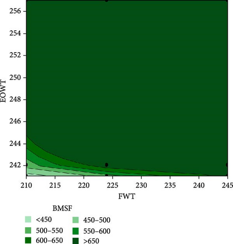
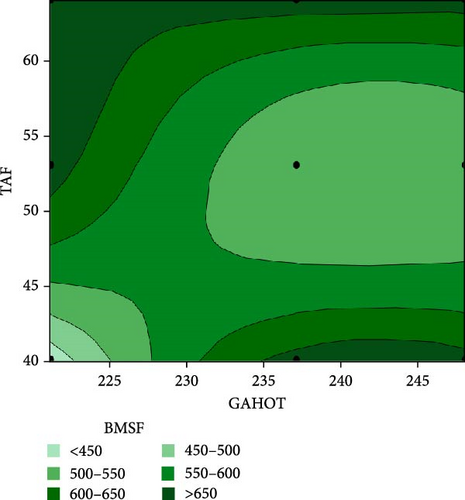
Contour plots are used to graphically represent the relationship among three variables in two specific dimensions at a time. Such plots are regularly used to establish desirable response variables and the input factors [60]. Minitab software normally plots the values for the input factors on the x and y axes, while contour lines and colored bands represent the values for the response variable. In this study, contour plots were constructed using statistical analysis software to evaluate the impact of the relationship between the selected design factors on BMSF. Figures 5 and 6 present the contour plots for BMSF with the interaction of four parameters’ involvement.
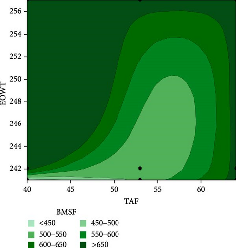
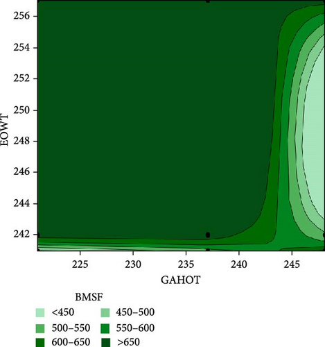
Contour plots for EOWT vs TAF and EOWT vs GAHOT are respectively presented in Figure 5a,b. Figure 6a shows that the interaction between the EOWT and TAF is quadratic, and as the EOWT increased from 242 to 256°C with the increase of the TAF from 50% to 64% air inlet flow, the BMSF increased from 450 to 650T/h. In Figure 5b, increase in EOWT and GAHOT brings about increase in BMSF. However, the value of BMSF decreases as GAHOT increased in value from 240°C. Study of such operating parameters interaction is essential in effective operation of boiler for sustainable power generation. In a situation when there is a drop in feedwater to the boiler due to unavailability of water from water source and insufficient inlet gas for igniting the furnace in the boiler unit, under this condition, the boiler unit may not generate superheated steam to power the turbine that would generate electricity (as temperature variation is very significant in the generation of quality steam in the steam boiler for power generation via steam turbines [61, 62]. When low-quality steam is being produced in boiler, such problem can easily be traced through the EOWT and GAHOT.
The interaction between EOWT and FWT is presented in Figure 6a. From the plot, it is seen that increase in EOWT and FWT favors the BMSF as this response variable increased. Figure 6b shows the plot of interaction between TAF and GAHOT. This plot reveals that increase in TAF and GAHOT does not favor BMSF as this decreased in value. Findings from this study shows that the TAF needs to be regulated between 45% and 50% of the air inlet to the furnace. The GAHOT constantly maintains temperature between 245 and 250°C to produce superheated steam in the boiler unit of about 541 to 690 L/h, which will flow to the HP turbine for power generation. It can be inferred from these plots that if the boiler system is not adequately monitored, the boiler system would deliver unsaturated steam to the turbine unit, this in turn will cause an increase in the failure rate of the turbine blade due to thermal corrosion [63, 64, 65].
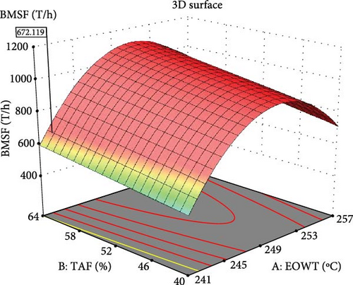
The interaction effect of operating conditions on BMSF using 3D surface plot is presented in Figure 7. From this plot, as both TAF and EOWT increased, BMSF also increased. This interaction favors the production of BMSF. From Figure 8, it can be seen that increase in the values of these two factors will increase the BMSF.
3.4. Numerical Optimization of Operating Conditions for BMSF and S/N Ratio
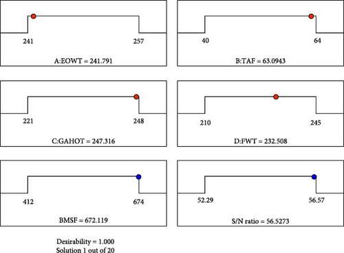
S/N ratio is a statistical measure used to measure performance in Taguchi technique [66]. S/N ratio helps in data analysis and prediction of optimum results. S/N ratio determines the influence of design parameters such as EOWT, TAF, FWT, and GAHOT on BMSF. In this study, MINITAB 18.0 software was used for the parameter settings with the highest S/N ratio, which always produces the optimum quality with lower variance. The highest value of BMSF is desirable for this study [67]. Hence, ‘Larger is the better’ type category of the performance characteristic for BMSF was selected to analyze the S/N ratio with results presented in Table 9. Table 9 presents 20 series of solutions for optimization of operating conditions (EOWT, TAF, GAHOT, and FWT). All the solutions provided by the Design Expert are feasible due to their desirability values of 1. For better optimum region for BMSF and S/N ratio, the desirability value of an optimum solution should be close to unity. The optimum solution 1 was selected by software as the optimum conditions as shown in Table 9. At optimal conditions of EOWT (241.791°C), TAF (63.094%), GAHOT (247.316°C), and FWT (232.508°C), optimal BMSF of 672.119 T/h and S/N ratio of 56.527 were obtained with desirability of 1 as shown in ramp plot (Figure 9).
| Optimum solution | EOWT | TAF | GAHOT | FWT | BMSF | S/N ratio | Desirability | |
|---|---|---|---|---|---|---|---|---|
| 1 | 241.791 | 63.094 | 247.316 | 232.508 | 672.119 | 56.527 | 1.000 | Selected |
| 2 | 256.756 | 42.547 | 228.665 | 231.188 | 603.621 | 55.308 | 1.000 | — |
| 3 | 256.364 | 41.787 | 225.385 | 224.982 | 570.919 | 54.718 | 1.000 | — |
| 4 | 256.792 | 56.688 | 229.497 | 214.023 | 603.685 | 55.495 | 1.000 | — |
| 5 | 241.959 | 50.832 | 224.236 | 234.071 | 668.707 | 56.309 | 1.000 | — |
| 6 | 242.884 | 42.541 | 234.293 | 227.447 | 653.853 | 56.086 | 1.000 | — |
| 7 | 255.323 | 45.951 | 224.303 | 222.383 | 652.555 | 55.935 | 1.000 | — |
| 8 | 242.984 | 47.624 | 221.119 | 210.531 | 596.570 | 55.072 | 1.000 | — |
| 9 | 256.203 | 43.325 | 224.546 | 237.005 | 656.508 | 56.048 | 1.000 | — |
| 10 | 256.811 | 49.285 | 235.474 | 222.315 | 646.058 | 56.055 | 1.000 | — |
| 11 | 244.638 | 40.228 | 230.982 | 210.098 | 656.006 | 55.914 | 1.000 | — |
| 12 | 241.900 | 41.350 | 221.675 | 211.969 | 500.728 | 53.575 | 1.000 | — |
| 13 | 241.015 | 57.351 | 242.743 | 221.517 | 509.995 | 54.212 | 1.000 | — |
| 14 | 256.975 | 52.372 | 227.279 | 228.675 | 626.646 | 55.802 | 1.000 | — |
| 15 | 254.535 | 40.304 | 227.509 | 212.955 | 633.548 | 55.520 | 1.000 | — |
| 16 | 242.000 | 53.000 | 248.000 | 210.000 | 513.431 | 54.254 | 1.000 | — |
| 17 | 242.000 | 40.000 | 237.000 | 245.000 | 670.917 | 56.493 | 1.000 | — |
| 18 | 256.960 | 51.184 | 221.552 | 242.351 | 654.554 | 56.223 | 1.000 | — |
| 19 | 241.280 | 50.536 | 234.048 | 222.075 | 524.068 | 54.312 | 1.000 | — |
| 20 | 243.679 | 48.937 | 226.454 | 212.165 | 653.149 | 55.978 | 1.000 | — |
The results of optimum BMSF and S/N ratio presented in Table 6 (generated by using MINITAB 18.0 software) are well comparable to those shown in Table 9 (generated by Design Expert software). This shows that the design factors have reasonable interactions to improve the BMSF and S/N ratio based on the quadratic regression models developed.
The optimum conditions corresponding to process levels are shown as the peak point as shown in Figures 8 and 10. Also, it can be seen that the levels of the design factors have reasonable interactions to improve the BMSF. From the graphical representation in Figures 8 and 10 the optimal factor combinations are 242°C of EOWT, 63% of TAF, 247°C of GAHOT, and FWT of 233°C, which give the maximum values of S/N ratio of 56.5 and 672 T/h of the BMSF. From this study, the combination ratio of the run factors of E3T3G 2F1 gives the optimized control conditions of the design factors for high performance of the BMSF for sustainable power generation of the selected steam turbine power plant.
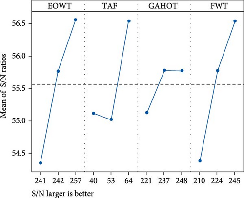
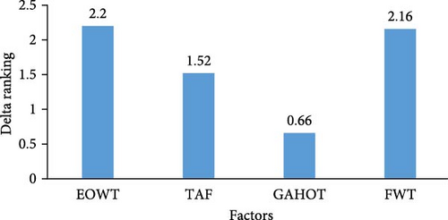
The delta S/N ratio and the percentage contribution ratio were employed to establish the best or the most influential design factor in assessing optimal performance of the BMSF. The most influential design factors were ranked in Tables 4 and 5. Figure 11 presents the ranking of the design factors. From Figure 11, EOWT contributed 38% with delta value of 2.2, which is ranked as the most influential factor on BMSF, followed by FWT with a contribution ratio of 36% and delta value of 2.16. Also, the TAF contributed 23% with a delta value of 1.52. Finally, the least influential factor is GAHOT with a contribution ratio of 3% and delta value of 0.66.
3.5. Interaction of Design Factors on the Mean BMSF and SNRA
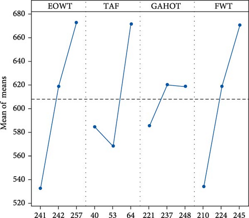
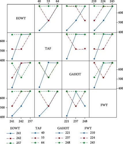
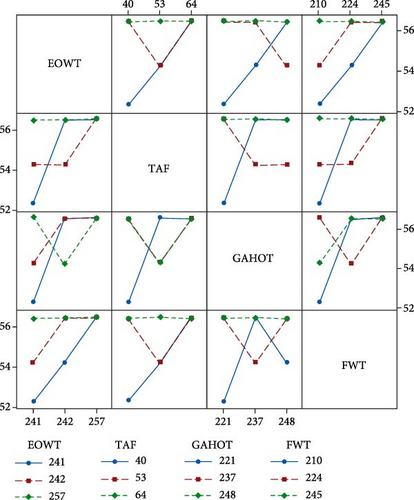
The mean response parameter and the mean S/N ratio based on the interaction of the design parameters are presented in Figures 12 and 13, respectively. The interaction plot demonstrates the relationship between a design factor and a continuous response which is BMSF. Parallel plots represent less interaction between the parameters, while intersecting plots indicate that interactions exist between the parameters. Studies have shown that the strength of the interaction plot is proportional to nonparallelism of the lines [68]. Moreover, it has been shown that in the interaction plots, the deviation from the horizontal line indicates the greater influence of the design parameter on the response factor [69]. From the interaction plots, there is minimum interaction between GAHOT and the response factor. Considering the S/N plot, it is obvious that the interactions between EOWT, TAF, and FWT are more significant. This is probably because the significance of these three design factors are more alike. Notwithstanding, the plots indicate that the levels of the three factors have reasonable interactions to improve the BMSF.
4. Conclusion
- •
The Taguchi design method has proven very reliable by the developed model in predicting the performance of the BMSF with 95.5% confidence level.
- •
The selected steam boiler will perform maximally if the optimal design factors are employed at 257°C of EOWT, 64% of TAF, 237°C of GAHOT, and FWT of 210°C at the boiler feed drum. These optimal design factors give the maximum S/N ratio of 56.57 and a maximum BMSF at 674 T/h.
- •
The most influential factor on the BMSF is the EOWT with a percentage contributing ratio of 38%, followed by FWT with 36%, and the TAF and GAHOT have a contributing ratio of 23% and 3%, respectively.
This study has future application to thermal power plants in the sense that, irrespective of the type and size of boiler, there are several factors, which are required to identify, analyze and control their impacts on boiler’s efficient operation and performance. Hence, this study is relevant to power plant engineers by providing information that will help to minimize heat losses in boiler such as radiation heat loss, conduction heat loss, convective heat loss, due to several factors in the process of generating steam. Moreover, a study of this nature will help to reduce the main cause that affect the performance of a boiler such as the generation of dry flue gas, the presence of excess air, the accumulation of carbon dioxide, and other emissions due to unburnt fuel by appropriate selection of the right combination of design factors.
Moreover, if these optimal design factors are considered in the selected steam power plant operation, the efficiency of the power plant will be enhanced significantly for sustainable power generation via the steam generated from the boiler unit.
Conflicts of Interest
The authors declare no conflicts of interest.
Funding
This research was funded by Taif University, Saudi Arabia, Project No. TU-DSPP-2024-91.
Acknowledgments
The author Bahaa Saleh extends his appreciation to Taif University, Taif, Saudi Arabia, for supporting this work through Project Number TU-DSPP-2024-91.
Open Research
Data Availability Statement
The authors declare that available data are included in the manuscript.


