Harnessing Principal Component Analysis and Artificial Neural Networks for Accurate Solar Radiation Prediction
Abstract
Accurate solar radiation prediction is essential for optimizing renewable energy systems and supporting grid stability. This study investigates the use of principal component analysis (PCA) for dimensionality reduction in solar radiation prediction models, followed by an evaluation of the models’ performance across varying feature sets. A series of case studies were conducted, comparing models using raw meteorological inputs with those employing reduced principal components (PCs) as inputs. Results demonstrate that while retaining fewer PCs reduces computational complexity, it can significantly affect model performance. The model with all meteorological inputs achieved the best results with an R2 of 0.99198, MSE of 562.612, and MAPE of 0.1899%. By contrast, the single-PC model exhibited an R2 of 0.11699 and MAPE of 64.5897%, highlighting the trade-off between dimensionality reduction and prediction accuracy. The study also emphasizes the computational efficiency gained through PCA, particularly in high-dimensional datasets. Future directions include integrating hybrid feature extraction techniques, leveraging advanced deep learning architectures, and exploring temporal and spatial dynamics to further refine prediction accuracy. The findings provide a roadmap for developing scalable and interpretable solar radiation prediction models, advancing their integration into real-time renewable energy systems.
1. Introduction
Accurate solar yield prediction is crucial for optimizing the performance of solar energy systems and improving the efficiency of renewable energy generation. As the demand for solar power continues to rise, precise prediction models are essential to minimize the uncertainty in energy production, which can be influenced by environmental factors, such as solar radiation, temperature, and cloud cover. Traditional methods of solar yield prediction, including statistical approaches and simple regression models, often fail to capture the complex, nonlinear relationships between these variables, leading to suboptimal accuracy in forecasting [1].
To address these challenges, machine learning (ML) techniques have become increasingly popular due to their ability to model complex and nonlinear relationships. Among these techniques, artificial neural networks (ANNs) have demonstrated strong predictive capabilities in various domains, including renewable energy prediction [2]. However, one of the primary challenges in applying ANN to solar yield prediction lies in the high dimensionality of the input data, which can lead to overfitting, increased computational cost, and poor generalization performance [3]. Principal component analysis (PCA) has proven to be an effective dimensionality reduction technique, enabling the transformation of a large set of correlated features into a smaller set of uncorrelated components, while retaining most of the data’s variance [4]. When combined with ANN, PCA can potentially improve model efficiency and reduce overfitting by identifying and retaining only the most significant features, while discarding irrelevant or redundant data [5].
Despite the individual success of PCA and ANN in different predictive modeling tasks, their integration in solar yield prediction remains an area with limited exploration. Some recent studies have explored the use of PCA for feature extraction in combination with ANN for solar radiation predictions [6] and energy load forecasting [7]. However, the combination of PCA and ANN for solar yield prediction has not been extensively studied, particularly with respect to the impact of dimensionality reduction on model accuracy and computational performance. This paper aims to investigate the effectiveness of using PCA for feature extraction and ANN for prediction, with the objective of improving solar yield prediction by reducing dimensionality while maintaining high prediction accuracy.
The remainder of this paper is organized as follows: Section 2 reviews related work on solar yield prediction and the use of PCA and ANN in energy forecasting. Section 3 presents the methodology, including the dataset, preprocessing steps, and model development. Section 4 discusses the results of the proposed models. Finally, Section 5 provides conclusions and suggests directions for future research.
2. Literature Review
The task of solar yield prediction has been extensively studied in recent years due to the growing importance of solar energy in the global renewable energy mix. Traditional prediction methods, such as statistical regression models, time-series analysis, and physical modeling, have been used to forecast solar power generation based on factors like solar irradiance, temperature, and humidity [3]. However, these methods often struggle to handle the complex, nonlinear relationships between input variables, which can result in lower prediction accuracy.
With the advent of ML techniques, ANNs have emerged as one of the most popular tools for solar yield prediction due to their ability to capture complex nonlinear patterns in data [8]. ANN models, particularly multilayer perceptrons (MLPs), have shown significant improvements in forecasting solar radiation and energy yield compared to traditional methods [9]. These models utilize multiple hidden layers and activation functions to approximate nonlinear mappings, making them well-suited for tasks where the relationship between input variables and output is highly intricate and difficult to model using linear techniques [10].
Despite their success, ANN models often face challenges related to the high dimensionality of input data. Solar energy datasets typically include a large number of features, such as various weather parameters (e.g., temperature, humidity, direct normal irradiance [DNI], diffuse horizontal irradiance [DHI], etc.) and time-related variables (e.g., time of day, season, and geographical location). The inclusion of many features can lead to overfitting, where the model captures noise in the data instead of the underlying patterns [11]. This issue often results in poor generalization performance and increased computational costs.
To address the dimensionality problem, PCA has been widely adopted as a dimensionality reduction technique. PCA transforms the original correlated feature space into a new set of orthogonal features, called principal components (PCs), that capture the most significant variance in the data [4]. By retaining only the PCs that account for the majority of the variance, PCA reduces the number of input variables for ML models without sacrificing much predictive power. This reduction can improve model efficiency, reduce the risk of overfitting, and simplify the training process [12].
Several studies have investigated the use of PCA in combination with ANN for various applications, including energy forecasting. In the context of solar energy, PCA-based feature extraction has been used to select the most relevant features and improve the performance of ANN models for predicting solar irradiance [13]. For example, in a study by Howley et al. [12], PCA was applied to reduce the dimensionality of weather data, and the transformed features were fed into an ANN for solar radiation forecasting. The results demonstrated that PCA-enhanced ANN models significantly outperformed traditional ANN models that used the original high-dimensional input data.
In addition, other dimensionality reduction techniques such as independent component analysis (ICA) and singular value decomposition (SVD) have also been explored for feature extraction in solar yield prediction. These methods, like PCA, aim to identify the most informative components of the data, though they differ in the mathematical approach and assumptions [14]. While ICA is more suited for situations where the data has non-Gaussian distributions, PCA remains the most commonly used method due to its simplicity and effectiveness in capturing the main variance in the data.
Although much progress has been made, challenges still remain in optimizing the integration of PCA with ANN models for solar yield prediction. Most studies focus on comparing the performance of PCA-based models against conventional ANN models or other ML techniques. However, there is a lack of consensus on how PCA impacts the model’s generalization performance and whether the improvements in accuracy justify the reduction in input dimensionality [15]. Additionally, the choice of ANN architecture, including the number of hidden layers, neurons, and activation functions, is often not standardized across studies, which can lead to inconsistent results.
Moreover, the combination of PCA and ANN for solar yield prediction has not been widely explored with respect to its application in real-time forecasting or integration into operational energy management systems. There is a need for further research to optimize the use of PCA for feature extraction in dynamic environments and to assess the scalability of these models when applied to large, real-time datasets [16].
This paper aims to contribute to the body of literature by exploring the effectiveness of PCA for feature extraction and ANN for solar yield prediction, specifically focusing on the impact of dimensionality reduction on prediction accuracy and computational efficiency. By comparing the performance of ANN models trained on original and PCA-reduced datasets, this study seeks to provide new insights into the role of dimensionality reduction in improving solar yield forecasting.
3. Methodology
3.1. Data Description
The dataset utilized in this study spans a period of 3 years (2014–2016), providing high-resolution, 1-min interval measurements of key solar radiation parameters: global horizontal irradiance (GHI), DNI, and DHI. These measurements were recorded at a location in Folsom, situated within the Sacramento metropolitan area in Northern California, with geographic coordinates ~38°40′43”N and 121°09′35”W. In addition to solar irradiance data, the dataset includes complementary information from numerical weather prediction (NWP) models and meteorological variables, such as temperature, humidity, and wind speed. These overlapping datasets provide a robust framework for capturing the intricate interactions between solar radiation and weather conditions. The combination of detailed solar and meteorological data allows for a thorough investigation of solar radiation patterns across different timescales, encompassing daily and seasonal variations. To ensure data quality and suitability for modeling, several preprocessing steps were applied. The original dataset comprised 1,048,575 records collected at a 1-min interval over the 3-year period. Missing values were handled using linear interpolation to maintain data continuity. To align with the temporal resolution typically used in solar radiation forecasting, the data were aggregated on an hourly basis. Additionally, nighttime records where GHI = 0 were excluded, as they do not contribute to solar radiation prediction. After these preprocessing steps, the dataset was reduced to 9462 records, which were then divided into training (80%) and testing (20%) sets for model development and evaluation. This structured approach ensures that the dataset remains representative while optimizing model performance.
This comprehensive dataset serves as an ideal foundation for modeling and predicting solar yield, offering insights into both short-term and long-term trends. The high temporal resolution of the data further enhances its utility, enabling the analysis of rapid fluctuations in solar radiation and their correlation with weather phenomena, thereby improving the accuracy and reliability of solar yield prediction models.
3.2. Data Preprocessing
3.2.1. PCA
The study begins with comprehensive data cleaning and preprocessing to ensure the accuracy and reliability of the dataset. This process includes imputing missing values and removing outliers, establishing a robust foundation for subsequent analysis. Once the data are prepared, PCA is employed as a dimensionality reduction technique. PCA is an unsupervised learning method that simplifies high-dimensional data into a lower dimensional representation, enhancing its interpretability while retaining essential information for analysis and visualization [17, 18]. By varying the number of PCs, the study explores the influence of dimensionality on ANN performance, aiming to identify the optimal trade-off between computational efficiency and predictive accuracy.
- •
It reduces the number of potentially correlated variables to a smaller, independent subset [19, 20].
- •
It decreases computational complexity and processing time.
- •
It eliminates irrelevant and noisy features from the dataset.
- •
It enhances overall data quality.
- •
It improves the accuracy and efficiency of algorithms.
- •
It facilitates data visualization in a reduced feature space.
- •
It boosts the performance of classification and regression tasks [21, 22].
This study begins with thorough data cleaning and preprocessing, including imputing missing values and removing outliers to ensure accuracy and reliability. This initial step establishes a solid foundation for precise analysis in subsequent stages. Following this, PCA is applied to streamline feature extraction. PCA, an unsupervised learning technique, effectively reduces high-dimensional data to a simpler form that is easier to manipulate, analyze, and visualize [17, 18].
Using different subsets of PCs, multiple ANN models are trained to assess how varying levels of dimensionality affect key performance metrics. The analysis also investigates the trade-off between preserving explained variance and reducing computational complexity. Results demonstrate the optimal number of PCs required for the best ANN performance, providing insights into the effectiveness of PCA in solar yield prediction. This approach highlights the versatility of PCA as a preprocessing technique, emphasizing its role in improving ANN efficiency and accuracy while enabling the systematic evaluation of feature dimensionality. Examples of PCA components and the selected features are detailed in Tables 1 and 2. Providing an overview of the transformation results.
| Timestamp | T (°C) | H (%) | Pr (h·Pa) | W-speed (m/s) | W-direction (degree) | Max_WP | P (mm) | DNI (W/m) | DHI (W/m) | GHI (W/m) |
|---|---|---|---|---|---|---|---|---|---|---|
| 1/2/2014 | 2.93 | 74.97 | 1009.83 | 1.66 | 171.86 | 2.24 | 0 | 88.45 | 7.26 | 12.94 |
| 1/3/2014 | 6.33 | 63.11 | 1010 | 0.66 | 114.69 | 1.14 | 0 | 631.31 | 39.01 | 146.65 |
| 1/4/2014 | 11.17 | 47.74 | 1010.13 | 0.62 | 248.09 | 0.98 | 0 | 709.66 | 68.39 | 287.12 |
| 1/5/2014 | 13.44 | 41.77 | 1010.42 | 0.83 | 278.28 | 1.28 | 0 | 782.01 | 66.27 | 390.23 |
| 1/6/2014 | 16.31 | 34.28 | 1009.67 | 0.85 | 241.01 | 1.39 | 0 | 863.02 | 60.27 | 469.5 |
| Timestamp | PC1 | PC2 | PC3 | PC4 | PC5 | PC6 | PC7 | PC8 | PC9 | GHI (W/m) |
|---|---|---|---|---|---|---|---|---|---|---|
| 1/2/2014 | −1.53 | 1.81 | −0.74 | −0.12 | 0.34 | −0.12 | −0.06 | 0.43 | −0.23 | 12.94 |
| 1/3/2014 | −1.58 | 0.01 | −1.29 | 0.81 | 0.64 | 1.07 | −0.98 | 0.57 | 0.03 | 146.65 |
| 1/4/2014 | −0.16 | −0.41 | −1.67 | 1.35 | 1.24 | −0.27 | −0.63 | 0.68 | 0.02 | 287.12 |
| 1/5/2014 | 0.51 | −0.26 | −1.7 | 1.28 | 1.48 | −0.4 | −0.51 | 0.61 | 0.02 | 390.23 |
| 1/6/2014 | 0.71 | −0.56 | −1.51 | 1.08 | 1.45 | 0.25 | −0.46 | 0.54 | 0.07 | 469.5 |
3.2.2. Efficiency Assessment
- •
RMSE evaluates the magnitude of prediction errors, penalizing larger deviations more heavily.
- •
MAE measures the average absolute difference between predicted and observed values, offering a straightforward interpretation.
- •
MAPE quantifies error as a percentage of the observed values, facilitating comparisons across datasets.
- •
MBE assesses the systematic bias of the predictions, indicating whether a model consistently over- or under-predicts.
- •
R2 measures the proportion of variance in the observed data explained by the model, with values closer to 1 indicating stronger predictive performance.
These metrics collectively enable a robust evaluation of the predictive capabilities and reliability of each model tested in the study.
3.3. Neural Network (NN) Development
The architecture of a NN consists of multiple interconnected layers of neurons, as depicted in Figure 1. During the training process, the biases and weights of the neurons are iteratively adjusted using optimization techniques to minimize prediction error, as described in [24]. The relationship between inputs and outputs within the NN can be expressed mathematically using Equation (10) [25]:
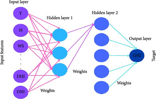
After conducting multiple pilot tests, the study determined that the most effective NN architecture for predicting GHI comprises an input layer, four hidden layers with 64, 512, 256, and 64 neurons, respectively, and an output layer with a single neuron dedicated to GHI prediction. To further enhance predictive performance, this optimized NN model is integrated with PCA for feature extraction and dimensionality reduction. This integration leverages the strengths of both PCA and NN to analyze the dataset efficiently and accurately. The results of this integrated approach, demonstrating its efficacy and impact on solar yield prediction, are detailed in the upcoming section.
3.4. Prediction Process
The proposed framework for solar energy prediction is structured into four key stages. The first stage involves data collection, where relevant solar energy data are gathered to create a comprehensive dataset for analysis. This dataset serves as the foundation for the predictive modeling process.
In the second stage, data preprocessing is performed to ensure the dataset is clean and suitable for modeling. This includes handling missing values, removing outliers, normalizing the data, and aggregating it on an hourly basis to align with the modeling requirements. These steps ensure that the input data are consistent and ready for use in subsequent stages.
The third stage is model training, where preprocessed data are used to train NN algorithms. During this phase, the models learn to recognize patterns and relationships within the dataset, enabling them to develop accurate predictive capabilities.
Finally, the fourth stage involves model testing and evaluation. In this phase, the trained models are assessed for accuracy and reliability using a separate testing dataset. This evaluation ensures that the models perform effectively on unseen data and can provide trustworthy predictions.
The entire process, from data collection to model evaluation, is systematically depicted in Figure 2, offering a clear overview of the methodology and its sequential steps.

4. Results and Discussion
The variance explained by each PC, as shown in Table 3, highlights their relative importance in representing the dataset’s variability. PC1, with an explained variance of 39.75%, is the most significant contributor, followed by PC2 (19.85%) and PC3 (12.69%). This suggests that the first three PCs capture the majority (~72%) of the dataset’s variance, making them highly informative for the predictive task. The diminishing variance from PC4 to PC9 indicates that these components contribute progressively less information and may be less critical for model training. This observation motivates the incremental reduction in input dimensions for the case studies, as illustrated in Table 4, where we defined all the cases explored in our investigation.
| Principal component | Explained variance |
|---|---|
| PC1 | 0.397516 |
| PC2 | 0.198547 |
| PC3 | 0.12692 |
| PC4 | 0.092933 |
| PC5 | 0.075476 |
| PC6 | 0.051769 |
| PC7 | 0.038788 |
| PC8 | 0.015533 |
| PC9 | 0.002519 |
| Case | Inputs | Output |
|---|---|---|
| a | Temperature, humidity, pression, windsp, winddir, max_windsp, precipitation, DNI, DHI | GHI |
| b | PC1, PC2, PC3, PC4, PC5, PC6, PC7, PC8, PC9 | GHI |
| c | PC1, PC2, PC3, PC4, PC5, PC6, PC7, PC8 | GHI |
| d | PC1, PC2, PC3, PC4, PC5, PC6, PC7 | GHI |
| e | PC1, PC2, PC3, PC4, PC5, PC6 | GHI |
| f | PC1, PC2, PC3, PC4, PC5 | GHI |
| g | PC1, PC2, PC3, PC4 | GHI |
| h | PC1, PC2, PC3 | GHI |
| i | PC1, PC2 | GHI |
| J | PC1 | GHI |
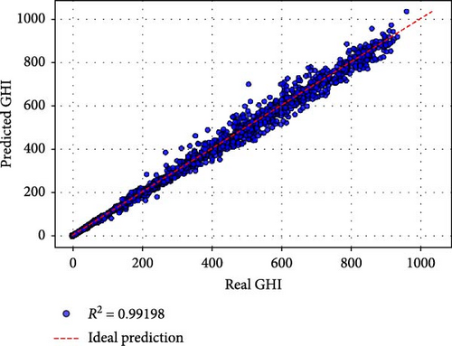
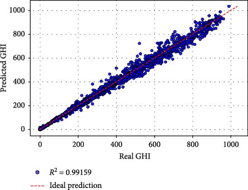
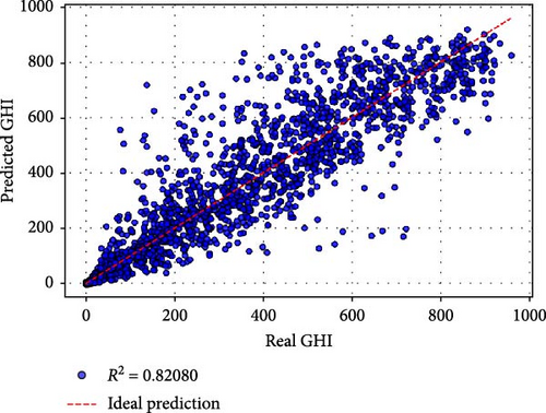
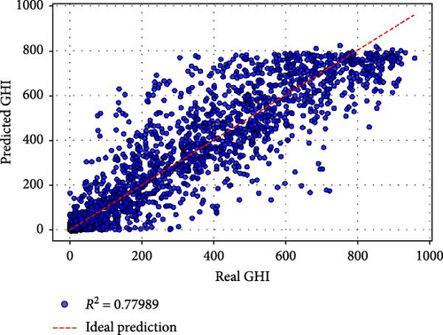
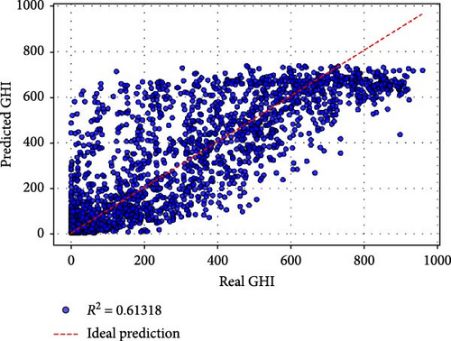
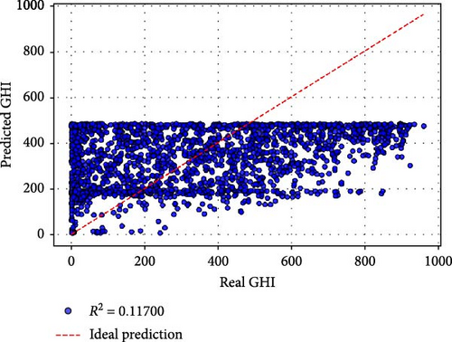
based on Table 5, Case a (all original were features used) achieved the best performance, with an MSE of 562.612, an RMSE of 23.719, and an R2 of 0.99198. The MAPE of 0.1899% and MBE of 2.078 demonstrate exceptional predictive accuracy and minimal bias. Training required 179.41 s over 94 epochs, reflecting a balance between computational efficiency and model complexity. The inclusion of all original features appears to provide the model with comprehensive information, resulting in superior performance. Case b utilized all nine PCs as inputs and yielded slightly lower performance compared to Case a. While the R2 of 0.99159 indicates excellent predictive capability, the MAPE increased to 0.4293%, and the training time rose to 231.79 s over 147 epochs. This suggests that while PCs effectively compress the information, the transformation may introduce a minor loss in interpretability and predictive precision. Cases c–e: Retaining six or more PCs (e.g., Case c with PCs 1–8 and Case e with PCs 1–6) maintained high R2 values above 0.97. However, the performance began to decline significantly in terms of MSE, RMSE, and MAPE, particularly in Case e (MSE: 1670.77, RMSE: 40.875, R2: 0.97619). Training times and epochs increased, indicating greater computational demands to fit reduced input spaces. Cases f–j: Retaining fewer than six PCs led to a pronounced drop in performance. For instance, Case f (PCs 1–5) had an R2 of 0.82080, and Case g (PCs 1–4) further deteriorated to 0.77989. The worst performance was observed in Case j (using only PC1), with an R2 of 0.11699, an MSE of 61955.913, and a dramatically higher MAPE of 64.59%. These results confirm that while PC1 captures the largest variance, additional PCs are critical for preserving sufficient information for accurate GHI predictions.
| Case | MSE | RMSE | R-squared | MAPE | MBE | Training time (s) | Number of epochs |
|---|---|---|---|---|---|---|---|
| a | 562.612 | 23.719 | 0.99198 | 0.1899 | 2.078 | 179.405893 | 94 |
| b | 590.215 | 24.294 | 0.99159 | 0.4293 | 0.682 | 231.788185 | 147 |
| c | 564.068 | 23.750 | 0.99196 | 0.3142 | −0.192 | 315.811647 | 247 |
| d | 682.345 | 26.122 | 0.99027 | 0.3167 | 3.993 | 338.209242 | 305 |
| e | 1670.770 | 40.875 | 0.97619 | 0.5754 | 4.741 | 495.685228 | 472 |
| f | 12,573.351 | 112.131 | 0.82080 | 0.5980 | −10.778 | 166.585155 | 80 |
| g | 15,443.813 | 124.273 | 0.77989 | 2.5443 | −6.071 | 237.033534 | 162 |
| h | 18,546.316 | 136.185 | 0.73568 | 7.1959 | −3.747 | 167.359929 | 102 |
| i | 27,141.639 | 164.747 | 0.61317 | 13.5462 | −12.078 | 126.686251 | 48 |
| j | 61,955.913 | 248.909 | 0.11699 | 64.5897 | 10.155 | 153.629068 | 76 |
- Note: Bold values were used the best metrics values among all the cases.
Interestingly, training time and the number of epochs required to converge varied across cases. Cases with fewer PCs (e.g., Case i with PCs 1–2) had shorter training times (126.69 s) but suffered from poor performance, suggesting that the computational savings come at the expense of predictive accuracy. Conversely, Cases b–d required longer training times, with Case d taking the most time (338.21 s). This underscores a trade-off between computational efficiency and model complexity.
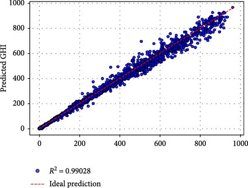
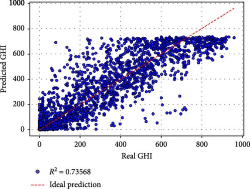
Figure 3 provides a visual comparison of the predicted and actual GHI values for different cases. Cases a and b exhibit tight clustering around the ideal prediction line, confirming their high accuracy. As PCs are reduced, the scatter widens, with Cases f–j showing significant deviations, particularly in the tails. This reflects the reduced capability of these models to capture the variance and dynamics of GHI with fewer input features.


The results demonstrate the utility of PCA as a dimensionality reduction technique. While using fewer PCs accelerates training, it also reduces predictive accuracy. For solar energy applications, where precision is paramount, retaining at least six PCs (Case e) appears to provide a reasonable balance between dimensionality reduction and accuracy. However, for critical scenarios, using all original features (Case a) remains the most effective approach.
The comparative evaluation underscores that the choice of input features significantly affects model performance. Cases with comprehensive inputs (original features or a large number of PCs) consistently outperform those with reduced dimensions. This is particularly evident in the stark contrast between Cases a and j. Furthermore, the computational trade-offs highlight the need to carefully balance model complexity against available resources.
These findings underscore the importance of input feature extraction and dimensionality reduction in solar radiation prediction models. Using PCA for dimensionality reduction can effectively compress data while maintaining high performance, particularly when retaining a sufficient number of PCs. However, retaining all original features yields the most accurate predictions. Future studies could explore hybrid approaches, combining PCA with feature selection techniques to further enhance model efficiency and precision.
5. Conclusion
This study investigated the impact of feature extraction and dimensionality reduction using PCA on solar GHI prediction models. The analysis demonstrated that while PCA effectively reduces the dimensionality of the dataset, the performance of the prediction models strongly depends on the number of PCs retained. Retaining all original features provided the highest accuracy, with Case a achieving the best performance metrics, including an R2 of 0.99198 and an MAPE of 0.1899%. However, reducing the number of PCs significantly degraded model performance, particularly when fewer than six PCs were used, as observed in Case j (R2 = 0.11699 and MAPE = 64.59%).
From a computational perspective, models with fewer PCs required less training time but at the cost of accuracy, highlighting a trade-off between computational efficiency and predictive performance. This trade-off is critical for solar energy forecasting applications, where precise predictions are essential for optimizing energy systems and planning.
Future research offers numerous opportunities to enhance solar radiation prediction models and their applications. Combining PCA with other feature selection methods, such as mutual information or recursive feature elimination, could improve model efficiency by focusing on the most relevant components while minimizing redundancy. Advanced NN architectures, such as convolutional neural networks (CNNs) or transformers, may better capture complex patterns in solar radiation data, especially with reduced feature sets. Incorporating temporal features like time of day and seasonality or spatial features like geographic location could further refine models, particularly for large-scale solar forecasting. Developing interpretable models to provide insights into the contributions of features or PCs would aid decision-makers in understanding the drivers of solar variability. Integrating these models into real-time forecasting systems and evaluating their performance under dynamic conditions would enhance their practicality. Additionally, extending this research to assess the impact of solar radiation predictions on photovoltaic system performance, battery storage optimization, and grid integration could significantly benefit renewable energy deployment. These directions collectively promise to improve the accuracy, efficiency, and applicability of solar radiation prediction models in renewable energy systems.
Conflicts of Interest
The authors declare no conflicts of interest.
Author Contributions
Conceptualization: Oussama Khouili and Mohamed Hanine. Methodology: Oussama Khouili and Mohamed Louzazni. Software, resources, data curation, writing–original draft preparation: Oussama Khouili. Validation, writing–review and editing, supervision: Mohamed Hanine and Mohamed Louzazni. Formal analysis, investigation, visualization, project administration: Oussama Khouili, Mohamed Louzazni, and Mohamed Hanine. All authors have read and agreed to the published version of the manuscript.
Funding
This research received no external funding.
Acknowledgments
AI has not been used in the preparation of the manuscript.
Open Research
Data Availability Statement
The data are available publicly in Carreira Pedro, H., Larson, D., and Coimbra, C. (2019). A comprehensive dataset for the accelerated development and benchmarking of solar forecasting methods (Version V1) (dataset). Zenodo. https://doi.org/10.5281/zenodo.2826939.


