Global climate change has intensified the search for renewable energy sources. Solar power is a cost-effective option for electricity generation. Accurate energy forecasting is crucial for efficient planning. While various techniques have been introduced for energy forecasting, transformer-based models are effective for capturing long-range dependencies in data. This study proposes N hours-ahead solar irradiance forecasting framework based on variational mode decomposition (VMD) for handling meteorological data and a modified temporal fusion transformer (TFT) for forecasting solar irradiance. The proposed model decomposes raw solar irradiance sequences into intrinsic mode functions (IMFs) using VMD and optimizes the TFT using a variable screening network and a gated recurrent unit (GRU)-based encoder–decoder. Our study specifically targets the 1-h as well as different forecasting horizons for solar irradiance. The resulting deep learning model offers insights, including the prioritization of solar irradiance subsequences and an analysis of various forecasting window sizes. An empirical study shows that our proposed method has achieved high performance compared to other time series models, such as artificial neural network (ANN), long short-term memory (LSTM), CNN–LSTM, CNN–LSTM with temporal attention (CNN–LSTM-t), transformer, and the original TFT model.

1. Introduction

The recent increase in power consumption due to population growth and the economy has also led to rising demand for energy resources [1]. This demand can be efficiently met if energy resources are managed efficiently. The depletion of fossil fuels, the impact of climate change, and the need for energy independence have emerged as pressing global issues. To address these concerns, there has been a large increase in demand for renewable energy sources such as solar and wind power [2]. As a major renewable energy resource, solar power is projected to become a primary power source in the future due to its abundance and minimal carbon emissions. Solar energy intensity differs across the globe, from the equator to polar regions [3]. Fortunately, the technology required for converting solar energy to electricity is widely available. Moreover, investment costs are projected to decrease by 59% by 2025 [4]. In addition, it is expected that cumulative electric power generation will increase to 36.5 kWh by 2040 [5].

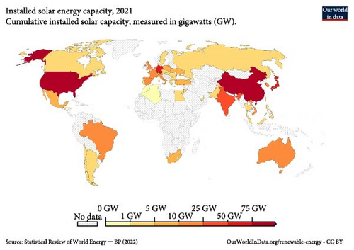
In 2018 [6], there was an 8% increase in the overall capacity of renewable power sources such as hydropower (increasing from 1112 to 1132 GW), solar (increasing from 405 to 505 GW), and geothermal power (increasing from 12.8 to 13.3 GW). Solar energy is an abundant source of energy that can be harnessed using solar photovoltaic (PV) panels to generate electricity from sunlight [7]. Currently, households and industries utilize solar PV technology to produce electricity [8], as it offers the advantage of quick energy production when there is sufficient sunlight. Additionally, installing solar PV systems is a cost-effective and convenient source [9, 10]. Nevertheless, the issue of producing electricity from solar PV panels persists, as various factors, such as partial or complete shading from clouds resulting in reduced power generation [11], deterioration of capacitors or batteries [12], potential induced degradation [13], and uncontrollable environmental factors [14], may hinder the process. The amount of electricity produced from solar panels is directly proportional to the global horizontal irradiance (GHI), which varies by time of day and location. The power output of solar panels is affected by meteorological conditions, resulting in intermittent production. Therefore, to integrate solar energy grids into existing infrastructures for grid stability and energy efficiency, it is crucial to have precise forecasts of GHI to account for the intermittent nature of solar power. Short-term forecasts are typically used to predict irradiation from 1h up to a week ahead, while long-term forecasts are utilized for predicting seasonal impacts on irradiation. Long-term forecasting is critical for financial planning and revenue generation, while short-term forecasting is crucial for managing utilities [15]. Figure 1 ¹ shows the amount of energy consumed in the year 2022 from solar. Lighter colors represent less energy consumed, whereas dark colors correspond to higher energy consumption.

Details are in the caption following the image — **Figure 1**
Open in figure viewer PowerPoint

The amount of solar energy consumed in 2022.

Energy forecasting refers to predicting the proportion of energy produced either from renewable energy sources (hydro, wind, and solar) or nonrenewable energy sources (natural gas, oil, and coal), referred to as fossil fuel sources. Forecasting energy-related tasks is of vast importance, as secure and cost-effective transmission is a major need today. Forecasting has played an important role in the power and energy industry as well as in business decision-making [16]. The world is facing significant challenges associated with forecasting, i.e., the intermittent and turbulent nature of these sources [17]. Intermittent solar energy and the amount of energy irradiance differ in different locations, e.g., hot regions experience longer daylight hours than cold regions.

These challenges have prompted a growing demand for renewable energy sources in large-scale energy systems and power grids as a cleaner and more sustainable alternative to traditional fossil fuels. Accurate forecasting can play a vital role in optimizing the utilization of renewable energy sources [18], as the integration of these sources with grid electricity has the potential to meet energy requirements more efficiently. Consequently, investments in renewable energy technologies have significantly surged, with many countries setting ambitious targets for deploying renewable energy to reduce greenhouse gas emissions and ensure energy security.

Numerous studies have been dedicated to developing advanced solar PV panels that can boost the production of electrical energy and enhance flexibility [19]. In addition to fixed models, portable solar PV panels have gained prominence and are being utilized in a variety of devices, including embedded Internet of Things (IoT) devices [20], electrical appliances, and monitoring sensors. The integration of computer programing technology has emerged as a critical aspect of solar PV operations, enabling efficient management and control of solar PV systems for optimal performance [21]. Forecasting, a subset of computer programing technology, involves predicting significant events and analyzing future trends. For instance, forecasting can be utilized to predict the deterioration of solar PV panels or solar irradiance [13], for predicting solar insulation using different deep learning techniques [22], and for forecasting regional energy consumption [23]. There is the ability to accurately forecast that solar irradiance has a positive impact on a solar PV system, leading to economic benefits. The objective of this study is to enhance the accuracy and dependability of solar irradiance predictions, even in instances of missing data. The occurrence of parameter malfunction resulting in missing solar irradiance readings is common and can be attributed to various factors, such as turbulent weather, device failure, signal interference, and uncontrollable circumstances. In this work, we investigate the performance of transformer-based architecture, namely temporal fusion transformer (TFT), and compare it with the various baseline methods. Furthermore, we present an enhanced TFT framework to improve the accuracy of mid-term hourly load time series forecasting. The main contributions of this paper are as follows:

•
We introduced an innovative and modified version of the TFT model that captures long-range dependencies for energy forecasting.
•
By combining variational mode decomposition (VMD) with TFT, our proposed model has achieved enhanced prediction accuracy by utilizing useful signals.
•
Our TFT model incorporates a variable screen network and a multihorizon fusion multihead attention module to provide insights into input–output relationships while retaining essential information. We replaced the long short-term memory (LSTM) encoder–decoder with a gated recurrent unit (GRU), enabling efficient learning of long-term temporal dependencies.

This paper is structured as follows: Section 2 presents related work. Section 3 describes the problem formulation and methodology adopted to forecast the hour-ahead solar irradiance. Section 4 describes the experimental settings, whereas Sections 5 and 6 discuss the baseline models and results and discussions, respectively. Finally, Section 7 provides the conclusion with future directions.

2. Related Work

In this section, we present the existing work in the literature related to energy forecasting.

Ma and Ma [24] proposed a renewable power generation and electric load prediction approach using a stacked GRU-recurrent neural network (RNN) based on AdaGrad and adjustable momentum. First, a correlation coefficient was applied to the input data for multiple sensitive monitoring parameter selection. Then, the selected parameters were input into the stacked GRU-RNN for accurate renewable energy generation or electricity load forecasting. In [25], a Bayesian deep learning-based probabilistic wind power forecasting model is proposed, using a fully convolutional neural network with Monte Carlo Dropout to construct precise prediction intervals (PIs). Using the Global Energy Forecasting Competition 2014 wind dataset, the model outperforms existing methods by providing accurate and narrower PIs, ensuring stable performance [26].. This is in contrast to conventional deep neural networks, which are deterministic and do not incorporate such uncertainties [27]. In [28], neural networks with a deterministic nature, as well as Bayesian neural networks (BNNs), were suggested for solar irradiation forecasting. In [29], Bayesian model averaging was utilized to predict the ensemble forecasting of solar power generation. Raza, Mithulananthan, and Summerfield [30] explored BNNs for load forecasting and found that due to the probability distribution of model parameters, BNNs take longer to converge compared to other probabilistic deep learning methods, resulting in larger dimensions.

A new machine learning-based method with the stationary wavelet transform (SWT) and transformers was presented for household power consumption forecasting [31]. The experimental findings suggested that the proposed approach outperformed the existing approaches. One disadvantage was that the system could fail under unknown circumstances. A transformer-based energy forecasting model was developed using Pearson correlation coefficient analysis to boost the prediction accuracy [32]. In [33], a comprehensive review of wind speed and wind power forecasting techniques using deep neural networks is conducted. It shows the potential of deep learning in improving forecasting accuracy. In [34], a detailed overview of the current state of wind speed and power forecasting, highlighting key methodologies and identifying areas to improve forecasting techniques to support the integration of renewable energy into power systems.

Wang et al. [17] presented a method for forecasting solar power output that relies on a deep feed-forward neural network. This approach utilizes data from multiple sources, including solar power and weather forecast data. Kim and Cho [35] predicted solar radiation intensity based on several kinds of weather and solar radiation parameters. An electricity forecasting model was developed using a hybrid CNN–LSTM architecture [36]. The CNN component was responsible for feature extraction, while the LSTM layer handled the temporal characteristics of the time series data. Additionally, a predictive model for energy consumption was proposed that utilized LSTM and the sine cosine optimization algorithm [37]. Kim and Cho [35] suggested a hybrid approach that merged a CNN and a bidirectional multilayer LSTM to create a sequential learning prediction model for energy usage. Additionally, another study introduced a similar hybrid model that combines a CNN and GRUs to improve the reliability of energy usage prediction. Both models utilized a coherent structure to achieve their respective goals. A similar model was presented by Real, Dorado, and Duran [38], in which a CNN–LSTM hybrid model was used for residential energy consumption forecasting. A hybrid architecture of CNN and artificial neural network (ANN) was proposed to exploit the advantages of both structures [39]. The proposed model was evaluated on RTE power demand data and a weather forecast dataset. In [40], short-term solar irradiance data were forecasted using 13 datasets from various sources worldwide, with a maximum forecast horizon of 15. The hidden Markov model was extended to an infinite space dimension. The experimental results demonstrated that the proposed model produced more stable forecasting results for higher horizons compared to those obtained from the Markov-chain mixture distribution model. Khan et al. [41] introduce AB-Net, a deep learning framework combining autoencoders and BiLSTM to forecast short-term renewable energy generation, achieving state-of-the-art results on benchmark datasets [40].

Numerous models have been extensively developed for time series forecasting owing to their great significance. Classical tools such as that in [42] serve as the foundation for many time series forecasting techniques. ARIMA [43] addresses forecasting challenges by converting a nonstationary process into a stationary one by differencing. In addition, a CNN-based model using sky images and past irradiance data can be developed to predict short-term solar energy fluctuations under different weather conditions [44]. DeepAR [45] is a forecasting technique that models the probability distribution of future series using a combination of auto-regressive techniques and RNNs. To capture both short- and long-term temporal trends, LSTNet [46] uses CNNs with recurrent-skip connections. Temporal attention is used by attention-based RNNs [47] to analyze long-range dependencies and make predictions. Moreover, a number of studies based on temporal convolution networks (TCNs) [48] use causal convolution to model temporal causation. The primary emphasis of these advanced prediction models is on modeling temporal relationships using techniques such as recurrent connections, temporal attention, or causal convolution.

In recent times, there has been a surge of interest in transformers [49], which leverage a self-attention mechanism to analyze sequential data, including those in natural language processing [50], audio processing [51], and computer vision [52]. Nonetheless, utilizing self-attention for forecasting long-term time series data poses a computational challenge due to the quadratic growth in both memory and time concerning the sequence length. The encoder–decoder framework, as implemented in the transformer model [52], employs an attention mechanism that allows the model to selectively consider relevant information, addressing the shortcomings of the sequence-to-sequence (Seq2Seq) model. This approach also enables parallel training, resulting in reduced training time. Fan et al. [53] presented a TFT that employs both a transformer structure and quantile regression (QR) to learn temporal properties and generate probability predictions. For global solar radiation prediction, Mughal, Sood, and Jarial [54] presented a time series model. The author developed three models, one was used for daily forecasting and the other two were used for hourly forecasting (including and excluding nighttime hours). Demir et al. [55] presented a variant of a transformer-based model for electrical load forecasting by improving the NLP transformer model. The results demanded the likelihood of developing a pretrained transformer model. Zhang et al. [56] introduced a transformer network that delivers highly precise solar power generation forecasts, surpassing the performance achieved with linear regression, CNN, and LSTM methods. A brief overview of related work is given in Table 1.

Table 1. Detailed literature review for solar irradiance forecasting.

Study	Objectives	Dataset	Evaluation measures
Dhillon et al. [57]	Solar energy forecasting in agricultural lands for efficient task scheduling of sensors	NSRDB solar power dataset	R2: 98.052 RMSE: 56.61
Nabavi et al. [26]	Energy forecasting using different machine learning models, in which NARX obtained good results	Energy consumption datasets of Iran	MSE: 0.149 RMSE: 0.495 MAPE: 1.87
Torres et al. [58]	Energy demand forecasting using deep learning techniques	RTE power demand data and weather forecast dataset	MAE: 808.316 MAPE: 1.4934 MBE: 21.7444 MBPE: 0.0231
Khan et al. [59]	Photovoltaic power generation prediction using a CNN–LSTM, a hybrid architecture	PV Rabat plant	MAE: 4.97 MAPE: 19.85 RMSE: 6.65
Kong et al. [60]	Energy forecasting using a CNN and GRU-based framework, AEP dataset, and IHEPC dataset	RTE power demand data and weather forecast dataset	MSE: 0.09 RMSE: 0.31 MAE: 0.24
Aasim, S. N. Singh, and Mohapatra [61] and Khan et al. [41]	Short-term renewable energy generation forecasting for efficient incorporation, merchandise management of energy deposits, and energy control systems	NREL wind dataset, solar power dataset	Solar dataset (MSE: 0.0106, RMSE: 0.1028); Wind dataset (MSE: 0.0004, RMSE: 0.0189)
Gaamouche et al. [62]	Electricity use and renewable energy plant production forecasting	PV datasets for two locations, Cocoa and Golden	Cocoa dataset (MAE: 0.035, MSE: 0.0023); Golden dataset (MAE: 0.034, MSE: 0.0027)
Xia et al. [63]	Electricity load prediction using a GRU-RNN	Hourly wind energy generation dataset	Wind dataset (RMSE: 0.0526, MAE: 0.0393); Load dataset (RMSE: 507.2, MAE: 351.5)
Kaur, Islam, and Mahmud [64]	RE forecasting using the integration of BiLSTM neural networks with compressed weight parameters using VAE, i.e., a VAE-Bayesian BiLSTM model	Solar generation time series data (2010–213)	RMSE: 0.0985 MAE: 0.0985 Pinball: 0.0386
Wu et al. [65]	Long-term energy usage forecasting using the transformer-based model	Six datasets: ETT	MSE: 0.06 MAE: 0.189
Wu et al. [49]	Global solar radiation prediction using a nonlinear autoregressive neural network model	NSRDB dataset	MAE: 0.93 RMSE: 1.28 MSE: 1.65
Devlin et al. [50]	Transformer long-term load forecasting	US utility company	2.571% MAPE accuracy increase
Dinculescu, Engel, and Roberts [51]	Energy usage forecasting using stationary wavelet transform (SWT) and transformers	UK-DALE: a domestic dataset of five distinct houses	RMSE: 0.0090 MAE: 00061 MAPE: 8.4765
Phan, Wu, and Phan [66] and Gao et al. [67]	Photovoltaic generation forecasting using a transformer-based model	PV power output from North Taiwan, with 1-h intervals and a range of 2 years	7.73% and 24.18% reduction in both NRMSE and NMAPE

Abbreviations: GRU, gated recurrent unit; LSTM, long short-term memory; MAE, mean absolute error; MSE, mean squared error; PV, photovoltaic; RNN, recurrent neural network.

In this paper, we present the modified version of TFT that is based on transformed architecture. Moreover, our proposed version of TFT incorporates VMD that captures the long-range dependencies in the data. We show the effectiveness of our proposed model by evaluating it on the solar irradiance dataset [42].

VMD offers superior decomposition capabilities compared to alternative methods like empirical mode decomposition (EMD) by overcoming issues such as mode mixing and providing better frequency separation, making it more robust for nonstationary signal analysis. Meanwhile, TFT excels in handling sequential data, offering better interpretability of time-varying features compared to classical methods like wavelet or Fourier transforms. TFT’s attention mechanisms also enable it to focus on critical temporal patterns, enhancing model performance in time-series tasks. These characteristics, along with their flexibility in various applications, justify their selection over other methodologies.

3. Methodology

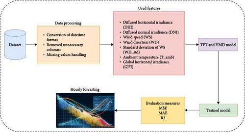
In this study, VMD and a TFT are adopted to forecast the N-hour-ahead solar irradiance. TFT [68] was proposed for time series forecasting, and in this work, some of its original components are modified to enhance the robustness of forecasts on longer time horizons. The forecasting workflow is illustrated in Figure 2. The workflow starts with raw data, and historical sequences and related features are extracted. The features of the dataset used are the same as those used by Haider et al. [42]. Data preprocessing is performed to ensure consistent data quality by removing unnamed columns, converting the “datetime” column to a proper datetime format, and handling missing values by averaging and filling in the missing entries. Then, the forecasting windows from which the model uses the past sequence and future horizon are created as well. The best hyperparameters obtained from the grid search were then used for training and testing using the different evaluation metrics. The modeling part comprises of statistical component VMD and a modified TFT. The model performance is analyzed using different performance metrics.

3.1. VMD

VMD is an advanced signal decomposition technique that is adaptive and nonrecursive. It can efficiently decompose nonstationary signals into a series of subpatterns with robust decomposition performance, allowing it to sufficiently address data noise. One of the major advantages of VMD is its fast and straightforward optimization process. The VMD method is utilized to extract multiple band-limited intrinsic modes concurrently from a complex signal. These intrinsic modes, known as intrinsic mode functions (IMFs), are AM-FM signals that represent the band-limited components of the original time series signal f(t). The following equation expresses the IMFs:

(1)

where u_k(t), A_t(t), and φ_K(t) refer to the IMF, instantaneous amplitude, and phase, respectively.

The analytical signal of each mode u_k(t) is computed by VMD using the Hilbert transform, which is then utilized to produce a one-sided frequency spectrum. The frequency spectrum of u_k(t) is then mixed with an exponent corresponding to the center frequency, shifting the spectrum to the baseband. The bandwidth of the demodulated signal is determined using the H1 Gaussian smoothness, which is the squared L2-norm of the gradient. The primary objective of VMD is to decompose the raw signal f(t) into multiple submodels (u_k(t), k = 1, 2, …, K) that each has a center frequency ω_k. The decomposition is subject to a constraint condition that the sum of all the modes must be equal to the raw signal. In VMD, the objective function minimizes the sum of each submodel’s frequency bandwidth that utilizes a constrained variational problem such that

(2)

where u_k and ω_k are the decomposed modes and the corresponding center frequencies, respectively, where k ranges from 1 to K. The symbol ∗ denotes the convolutional operator, t represents time, t = −j/2, and δ represents the Dirac distribution.

By using t, the confined problem is equivalent to the unconstrained problem. On the other hand, alpha ensures that the submodel can be reconstructed accurately, even in the presence of Gaussian noise. The unconstrained problem can be expressed as follows:

(3)

The alternating direction method of multipliers is used to solve u_k and ω_k through Equations (4) and (5).

(4)

(5)

Equation (5) is used to update the center frequencies, ω_k, while Equation (6) is used to update λ simultaneously. By utilizing the alternate direction method of multipliers as a foundation, the iteration stops once the termination condition, as given by Equation (7) and represented by ɛ, is achieved.

(6)

(7)

The real part of

, obtained through Fourier transform, is used to convert the final output of VMD, which is represented by

. The definition of r_res can be expressed as follows:

(8)

The raw wind speed (WS) data are represented by f(t), with Ns denoting the sample number and K representing the number of decomposed submodels. The decomposed modes are represented by u_kt. To determine the number of patterns, r_res should not exhibit a noticeable decreasing trend [69].

3.2. TFT

Transformer-based models with an encoder and a decoder have grown in popularity in time series forecasting [32]. The time series past data are fed into the encoder, and the decoder uses autoregressive forecasting to predict future values, leveraging an attention mechanism to focus on the most valuable historical information for prediction. Nevertheless, past approaches frequently ignore various input types or presuppose that all external inputs will be known in the future. TFT, on the other hand, model created especially for multihorizon time series forecasting [66]. TFT addresses these issues by matching structures to certain data properties, providing better than that of black-box models such as neural networks or complicated ensembles that conceal the relative relevance of features and their interactions. Furthermore, TFT represents a novel approach that surpasses other state-of-the-art forecasting models.

To assure good prediction performance with various forecasting issues, the TFT model architecture, which is shown in Figure 3, uses established components to build feature representations for each input type (i.e., static, known future, and observed inputs). There are separate inputs of the time-related input features X_{s,t−Ti:t−1} and X_s,t:t+To−1 with no shared parameters. Long-term time series temporal information is effectively handled by multilayer GRU encoders and decoders after the inputs X_{s,t−Ti:t−1} and X_s,t:t+To−1 are transformed. The proposed model replaces the usual LSTM layers in the TFT model’s encoder and decoder with GRU layers. One significant advantage of GRU is the unification of the forget and input gates into a single update gate, which allows it to more efficiently capture short-term dependencies and properly simulate sequences with rapid changes. The encoder and decoder outputs from the final layer are combined into a multi-timestep fusion module that distributes weights according to importance. By minimizing the revised quantile loss function, predicted quantile values are obtained. Note that modules with the same color in Figure 3 have the same parameters. TFT is made up of five main parts, which are broken down into gating mechanisms, variable screening networks, GRU encoder-decoder, multihorizon fusion, and PIs.

The TFT captures both short-term and long-term patterns, handles mixed data types, and offers interpretability through attention mechanisms. VMD decomposes signals into IMFs with minimal mode mixing and is robust to noise, making it ideal for nonstationary and complex time series data. Both models enhance time series forecasting by effectively processing intricate patterns.

3.2.1. Gating Mechanism

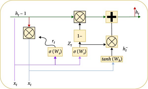
The gradient disappearance problem in RNNs is solved by the GRU’s use of temporal information processing, which retains pertinent information and discards irrelevant information. This system comprises a reset gate and an update gate. Although the update gate stores memory from the previous time step, the reset gate merges fresh input data with previous memory. An illustration is shown in Figure 4.

The GRU structure is described as follows:

(9)

(10)

(11)

The gated residual network (GRN) is integrated as a block of TFTs to provide the appropriate nonlinear structure to the model. The GRN input consists of two vectors, the primary information vector p and the context information vector c. The GRN computation is defined in Equation (9), and the ELU activation function is defined in Equation (11), where η₁ and η₂ are the outputs of two intermediate layers.

The gated linear units (GLU) play a vital role in achieving gate control functionality. The form of the GLU when the input is y is shown in Equation (12), where σ(.) are the sigmoid activation functions, and W( ) and b( ) are the weights and biases, respectively. As illustrated in Figure 5, the GRN uses the GLU to control the model structure and discard unnecessary layers. With the GLU, the GRN can regulate the model structure and avoid unnecessary layers.

(12)

3.2.2. Variable Screening Network

This module is used to select relevant input at each time step. The module’s structure is depicted in Figure 6.

represents the input vector of k features at time t, and cs is the context vector obtained by the gated residual processing of the static covariates.

(13)

(14)

(15)

(16)

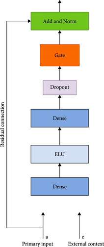
The input feature multihead attention module in Figure 6 weighs the input variables with weight vector h_t. The importance of each input feature is represented by h_t through the sigmoid activation function σ(.) and the intermediate variable. The ELU activation function is used instead of RELU to alleviate gradient disappearance. The module includes dropout, layer normalization, and softmax layers. The larger the weight h_t is, the more important the corresponding input variable is to the output.

3.2.3. Multi-Timestep Fusion

The multi-timestep fusion module is designed to capture long-term correlations in hourly load forecasting. It produces a vector with the expected size by allocating weights to all of the encoder and decoder outputs from prior time steps. This enables the model to concentrate on more crucial data. Figure 7 depicts the multihead fusion module structure.

To record long-term correlations between time steps, TFT makes use of self-attention. The values V are scaled by the modified transformer-based multihead attention mechanism according to the connections between questions Q and keys K. A multihead attention structure is used by the TFT to learn long-term time series correlations. Equation (17) is a definition of the self-attention mechanism, where Q, K, and V stand for the query, key, and value, respectively. With the relationships between queries QɛR^Nχd and keys KɛR^Nχd as a basis, attention mechanisms scale values as follows:

(17)

The linear transformation on the matrices Q, K, and V used in the self-attention mechanism is obtained by multiplying the input matrix X by the corresponding linear transformation matrices w_q, w_k, and w_v. The output matrix of the self-attention mechanism is then determined using these matrices. The typical multihead attention technique, repeated self-attention, can be used to create several sets of Q, K, and V matrices. For attention values, the scaled dot product is calculated as follows:

(18)

The proposed multihead attention distributes the matrix V among each head to address this, allowing the overall significance of a feature to be assessed, and h_m multihead attention is needed, where h_m is the number of heads and W^h differs for each head. Multihead attention uses several heads for various representation subspaces to increase the learning capacity of the attention mechanism.

(19)

(20)

where

and

refer to head-specific weights. As each head employs unique values, attention weights alone cannot accurately represent the significance of a specific feature.

(21)

(22)

(23)

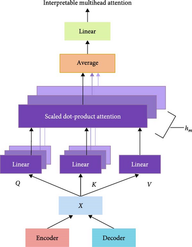
The equation above depicts the multihead attention mechanism, where A(.) represents a normalized function, and n is the dimension of the K vector. The weight matrices of Q and K for the hth head are denoted by and , respectively, while W_V represents the weight matrix of V shared across all heads to enforce time series causality.

3.3. Loss Function

The TFT predicts point predictions and quantile intervals simultaneously, where three percentiles, 10th, 50th, and 90th, are predicted at each step using the temporal fusion decoder’s linear transformation. The quantile loss is jointly minimized during training. The outputs of all quantiles are subsequently summed using the formula:

(24)

(25)

The weight parameters (W) of the TFT are optimized by jointly minimizing the quantile loss over the set of output quantiles (Q) and the training data domain (U), which consists of M samples.

4. Experimentation

In this section, we will explain the dataset and the process through which we conducted our experiments.

4.1. Dataset

The efficiency of solar PV energy systems is affected by numerous factors, including the location and weather conditions of the installation site. These factors can be broadly categorized into two groups: spatial factors and temporal factors. Spatial factors refer to the physical characteristics of a solar PV plant, such as its size, panel arrangement, and orientation, while temporal factors relate to variations in weather and climate conditions, including seasonal changes, weather events, and time of day.

Both spatial and temporal factors play an important role in determining the amount of solar energy that a PV system can generate. For instance, a larger solar PV plant with more panels will generally generate more energy than a smaller system, while the orientation of the panels and the arrangement of the plant can also impact its efficiency. Additionally, variations in weather and climate conditions can significantly affect the efficiency of PV systems, with factors such as cloud cover, temperature, WS, and humidity all playing a role.

In this study, we used a solar energy irradiance dataset [42], which is numerical data and it contains various parameters related to PV generation, such as GHI, diffused horizontal irradiance (DHI), and diffused normal irradiance (DNI), as well as WS. This dataset was collected over 5 years, from 2015 to 2019, at an EMAP tier 1 meteorological station located 500 m above sea level at 33.64 ° N and 72.98 ° E. The dataset consists of hourly records, and ~41,000 records are available for analysis. By examining the data and analyzing the various spatial and temporal factors that impact PV efficiency, the researchers sought to better understand how to optimize solar energy generation in this region. A detailed description of dataset variables is given in Table 2. We have used the same criteria of feature extraction adopted by Haider et al. [42], in which DHI, DNI, WS, wind direction (WD), and its standard deviation (WD_std) and ambient temperature (T_amb) were selected because of high correlation with GHI.

Table 2. Summary of statistics.

Statistics	GHI	DNI	DHI	T_amb	RH	WS	WS_gust	WD	WD_std	BP
Mean	197.5	177.6	88.42	21.9	59.02	1.77	4.18	175.1	13.0	944.7
Std	278.	301.8	127.9	8.48	20.82	1.38	2.47	108.2	10.0	9.573
Min	0.000	0.000	0.00	1.0	10.0	0.0	0.0	0.0	0.0	881.0
Max	1040.0	2777.0	843.	45.3	100.0	13.20	31.0	360.0	82.2	1002.0

Note: Minimum (Min), Mean, maximum (Max), and standard deviation (Std) values of all the daily parameters measured: global horizontal irradiance (GHI) in Wm⁻², diffused normal irradiance (DNI) in Wm⁻², diffused horizontal irradiance (DHI) in Wm⁻², ambient temperature (T_amb) in °C, relative humidity (RH) in %, wind speed (WS) in ms⁻¹, maximum WS within a specific time interval (WS_gust), wind direction (WD) in °N (to east), WD standard deviation (WD_std) and barometric pressure (BP).

4.2. Data Split and Preprocessing

Before feeding the data into each of the test models, we performed a data check to identify any missing values and the quantity of missing data. Additionally, during exploratory data analysis, a significant number of GHI values equal to zero were discovered. These zero values correspond to nighttime solar GHI values and were expected to be zero. However, this large number of zero values impacted the accuracy of the models, as there are 19,403 GHI values, while there are ~41,000 total records. To address this issue, all values between 7 p.m. and 5 a.m., the typical nighttime hours, were removed from the dataset, resulting in a reduction in the number of zero values to 4236. Then, the remaining missing values are treated as replacing with the average values. After selecting data for a specific time interval, the total number of records available for analysis was 25,785. This process ensured transparency in the dataset being used for modeling, thus improving the reliability of the results obtained from the models. The dataset was split into three subsets: a training set consisting of 70% of the data and a validation and test set consisting of 15% of the data each.

4.3. Training Details

For time series forecasting, a window is defined that consists of two values, the number of time steps taken to forecast the future value and the future values that are to be forecasted. Our experiments involved the use of four forecasting windows, each with a specific size. The sizes of these windows were (7,1), (14,3), (28,7), and (56,14), where the first number represents the number of past sequences and the second number represents the number of future sequences that the model needs to predict.

Since the data sequences are hourly based, the model uses a historical data sequence of a specific number of hours and forecasts future values for certain hours. For instance, in the first window size tuple (7,1), the model uses a past sequence of 7 h to predict the next hour’s sequence. Similarly, the model uses past sequences of 14, 28, and 56 h and predicts 3, 7, and 14 h into the future, respectively. We excluded zero-value transactions from the data between 7 p.m. and 5 a.m.; thus, 14 h of data sequences remain. Therefore, a day comprises 14 h. Hence, forecasting using window sizes (7,1) and (7,3) means predicting solar irradiance based on a half-day sequence, while forecasting using window sizes (28,7) and (56,14) involves taking 2- and 4-day past sequences to forecast the next half- and full-day solar irradiance, respectively. The best results were recorded based on the second-mentioned window. Different experiments were conducted with different training hyper-parameters, but the architecture of the TFT model used had the same settings, such as the number of layers, as in its original implementation. We experimented with different batch sizes, i.e., 16, 24, 32, 64, and learning rates between 0.0001 and 0.1. The quantile loss with seven quantiles was used as a loss function. We trained each model for 100 epochs using the Adam optimizer. The best validation model was used for testing purposes.

The models were implemented with a Ubuntu system using Python 3.8 with PyTorch. To split the data, the Time Series Dataset module was utilized. Early stopping was employed to prevent overfitting. The training for the TFT model was performed using a 1080 Ti (R) Core (TM) i7 GPU with 128 GB RAM.

5. Baseline Models

In this section, we present the baseline methods for our proposed model. We experimented with different settings, such as the number of layers and hidden units. Final configurations are given in the related subsections.

5.1. LSTM

LSTM is an improved RNN that is widely used for time series forecasting and solar irradiance [37]. This study used three layers of LSTM, with 64, 32, and 16 hidden units, and one dense layer, with 1, 3, 7, and 14 neurons for window sizes of (7,1), (14,3), (28,7), and (56,14), respectively.

5.2. ANN

ANNs consist of input, hidden, and output layers, with the hidden layer learning about data patterns through neurons. The hidden layer then forwards the result to the output layer. ANNs have self-learning capabilities and rely on data experience to learn and predict results. In this experiment, two ANN hidden layers, with 256 and 128 hidden units, and one dense layer for output, with 1, 3, 7, and 14 neurons for windows sizes of (7,1), (14,3), (28,7), and (56,14), respectively, were used.

5.3. Original TFT

Transformer-based models, comprising encoder and decoder parts connected via an attention mechanism, are well-known in time series forecasting. The encoder uses historical data as input, while the decoder predicts future values by focusing on valuable historical information. The decoder uses masked self-attention to prevent future value acquisition during training. However, previous methods do not consider different input types or assume that all exogenous inputs are known in the future. The original TFT [69] addresses these issues by aligning architectures with unique data characteristics via appropriate inductive biases.

5.4. GRU

GRU is also an RNN, and it can also be used as a solar irradiance model [63]. This study used three layers of GRU, with 64, 32, and 16 hidden units, and one dense layer, with 1, 3, 7, and 14 neurons for window sizes of (7,1), (14,3), (28,7), and (56,14), respectively.

5.5. CNN–LSTM

CNN–LSTM is a hybrid architecture consisting of LSTM layers stacked after CNN layers. Some recent studies have used such architecture for time series forecasting as well [37]. This study used two layers of CNN, with 32, and 16 hidden units, two LSTM layers with 16 hidden units each, and one dense layer, with 1, 3, 7, and 14 neurons for window sizes of (7,1), (14,3), (28,7), and (56,14), respectively.

5.6. CNN–LSTM With Temporal Attention (CNN–LSTM-t)

This study uses a CNN–LSTM model augmented with a temporal attention mechanism. The CNN layers are employed for local feature extraction from the input data, while the LSTM layer captures long-range dependencies and temporal patterns. The attention mechanism dynamically weighs the importance of different time steps in the LSTM output sequence, allowing the model to focus on relevant information. The CNN–LSTM-t used in this study consists of one Convolutional layer followed by a MaxPooling layer and a flattened layer. This is followed by an LSTM layer followed by an attention module with one Dense layer and additional layers for reshaping, applying activation functions, and performing element-wise multiplication. At the end, one dense layer, with 1, 3, 7, and 14 neurons, was applied for window sizes of (7,1), (14,3), (28,7), and (56,14), respectively.

5.7. Vanilla Transformer

Transformers are cutting-edge models in domains of different domains of artificial intelligence, including time series prediction that outperform typical deep learning architectures [70]. This study uses a vanilla transformer model with two heads of multiheaded self-attention followed by two dense layers, one with 1, 3, 7, and 14 neurons for window sizes of (7,1), (14,3), (28,7), and (56,14), respectively.

6. Results and Discussion

In this section, the performance of the proposed TFT, baseline models, and original TFT models is analyzed with varying forecasting window tuples, i.e., (7,1), (14,3), (28,7), and (56,14). The first value in the tuple represents the number of past time steps used for forecasting, where each step is 1 h, while the second value represents the number of time steps being forecasted, which is also 1 h. A window size of (4,1) is a single-step forecast, while the others are multistep forecasts ranging from 3 to 14 h ahead. As the dataset has zero values of GHI from 7 PM and 5 AM, the solar day becomes 14 h. Hence, a window size of (56,14) means using the past 4 days of data as input and forecasting the next day’s data. The dataset used [42] in this study contains GHI data as well as weather data in which temperature, WS, etc., are variable quantities and metaphorical features.

6.1. Baseline Models

Each model underwent rigorous training over 100 epochs for each window size, employing a batch size of 64 and utilizing mean squared error (MSE) as the chosen loss function. The model architecture featured two hidden layers, ensuring the capacity to capture and leverage temporal dependencies within the data. As the window size increased from (7,1) to (56,14), we observed a consistent trend of increasing loss values, indicating that larger window sizes allowed the model to capture more extensive contextual information except for CNN–LSTM, GRU in which loss decreased as window size increased. The loss was irregular for the model CNN–LSTM-t and transformer. This progression towards larger window sizes was accompanied by the continued utilization of two hidden layers, highlighting the model’s adaptability and efficiency in accommodating the expanded context.

6.2. Proposed TFT Models

This section presents the training and evaluation performance with the training and validation sets, respectively. In Section 5.4, we briefly introduce the metrics used to evaluate the models. The training and validation loss plots of the proposed TFT model are given in Figure 8 for window sizes of (7,1), (14,3), (28,7), and (56,14). The loss graphs show that the performance starts decreasing upon lengthening the forecasting window size.

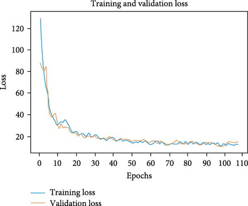
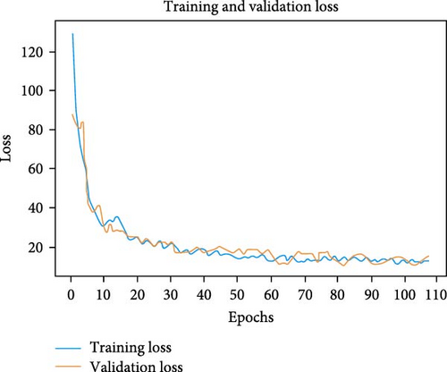
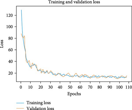
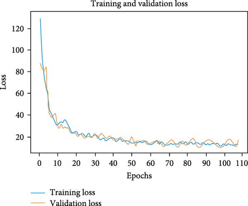
Conducted a systematic investigation by employing different window sizes, batch sizes, learning rates, layers, loss functions, and optimizers. The aim was to identify the combination that yields the most optimal results for our forecasting task. Notably, among the evaluated window sizes of (28,7), (14,3), and (56,14), the window size of (56,14) emerged as the most suitable choice, demonstrating superior performance across multiple configurations. This central window size effectively captures the necessary historical and contextual information, resulting in more accurate predictions. Consequently, we focused our subsequent analyses and optimizations primarily on the (56,14) window size, discarding configurations with lower performance potential. By strategically narrowing our focus to the optimal window size, we were able to achieve significant enhancements in the accuracy and efficiency of our forecasting model.

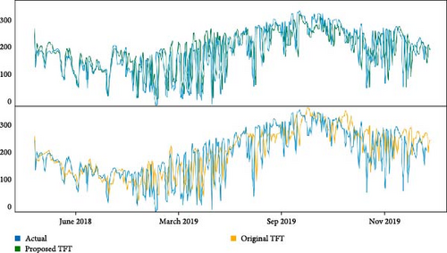
Figure 8 shows the performance of the proposed TFT with the actual irradiance value and shows the effectiveness of our methodology, mainly the GRU-based encoder and decoder, variable screening network, and feature fusion multihead attention mechanism.

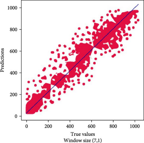
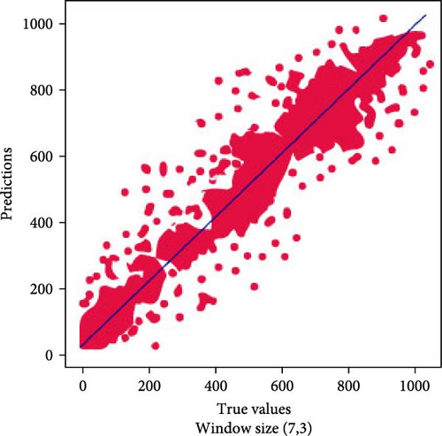
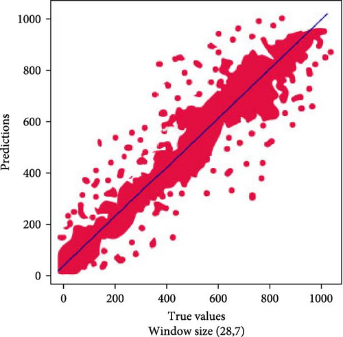
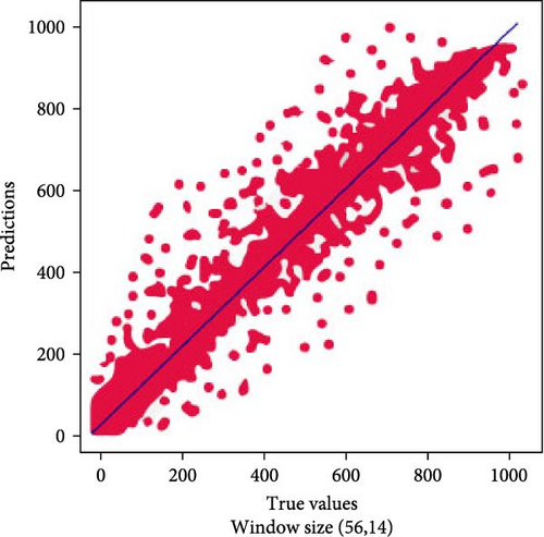
Figures 9 and 10 show the scatter plots for our proposed models on different window sizes. These plots provide valuable insights into the dispersion of prediction errors. Notably, for the window size (7,1), the points on the scatter plot exhibit a more scattered distribution, indicating a wider range of prediction errors. In contrast, the (14,3) window size shows points that are slightly more clustered, suggesting a more consistent performance. Moving to larger window sizes, such as (28,7) and (56,14), we observe an increasing dispersion of points, signifying a wider spread of prediction errors. This analysis highlights how the choice of window size can impact the reliability and consistency of our forecasting models, with smaller window sizes tending to produce more concentrated predictions and larger window sizes leading to a broader range of forecasting accuracy.

6.3. Performance Comparison

This section presents the comparative performance analysis of the proposed TFT, original TFT, LSTM, and ANN models in terms of all four performance metrics, mean absolute error (MAE), R2, MSE, and standard deviations (SD), and all forecasting window sizes, (7,1), (14,3), (28,7), and (56,14). For forecast horizon (7,1), it can be seen that our proposed model has outperformed the original TFT and other models significantly, with an MAE score of 19.29 and an R2 of 0.992, while the ANN also surpasses the original TFT and LSTM models in 1-h ahead prediction, with an MAE of 21.53 and an R2 of 0.981, while MAE values of 22.81 and 25.21 and R2 values of 0.971 and 0.926 are obtained using the original TFT and LSTM models, respectively. For 3-h ahead, forecasting, the proposed TFT and original TFT models have better performance compared to the LSTM and ANN models, with MAE values of 22.55, 24.28, 27.74, and 29.34, respectively, and R2 values of 0.978, 0.960, 0.902, and 0.895, respectively. From the 1-h prediction to the 3-h horizon, the original TFT and LSTM models perform better than the ANN model; however, the performance of both TFT models is approximately similar. This result shows the effectiveness of the transformer models in capturing long-range dependencies and, hence, perform well on the horizon of the window. In other words, the performance of the ANN and LSTM models deteriorates as the prediction horizon lengthens, as seen by a comparison of their R2 scores at various forecast horizons in Figures 9 and 10. For forecasting window sizes of (28,7) and (56,14), the proposed TFT has R2 scores of 0.940 and 0.921 R2, respectively, while the original TFT has R2 scores of 0.905 and 0.892, respectively. On the other hand, the LSTM and ANN models show deteriorating performance as the forecasting horizon length increases, with R2 scores of 0.882 and 0.831 for a window size of (28,7) and 0.835 and 0.818 for a window size of (28,7). Based on the performance of all models, it can be established that the ANN and LSTM models are highly effective in terms of short-term forecasting. However, as the forecast period becomes longer, the accuracy values tend to decrease. This is evident from the findings presented in Table 3, which displays the performance of each architecture across different forecast horizons.

Table 3. Comparison of the proposed method with the baseline models.

Model	Window size	MAE	MSE	R2
LSTM	(7,1)	25.21	1619.70	0.926
ANN		21.53	1251.51	0.986
CNN–LSTM		56.5	6424.7	0.588
CNN–LSTM-t		46.492	4415.06	0.7171
GRU		52.35	5289.3	0.661
Transformer		46.62	4310.5	0.723
Original TFT		22.81	1048.81	0.971
Proposed TFT		19.29	957.10	0.992

LSTM	(14,3)	27.74	1883.52	0.902
ANN		29.3	1937.99	0.895
CNN–LSTM		50.81	5230.6	0.665
CNN–LSTM-t		50.54	4800.8	0.6925
GRU		51.9	5214.6	0.666
Transformer		50.92	5194.6	0.667
Original TFT		24.28	1384.27	0.960
Proposed TFT		22.55	1242.34	0.978

LSTM	(28,7)	79.20	5624.07	0.882
ANN		95.84	7850.51	0.831
CNN–LSTM		52.6	5160.6	0.669
CNN–LSTM-t		49.2	4756.3	0.6956
GRU		49.2	4783.7	0.693
Transformer		48.5	4733.6	0.697
Original TFT		46.64	4918.68	0.905
Proposed TFT		41.08	3742.34	0.940

LSTM	(56,14)	94.60	8606.80	0.835
ANN		129.71	11,029.39	0.818
CNN–LSTM		51.7	5134.4	0.671
CNN–LSTM-t		50.76	4813.71	0.691
GRU		55.21	5805.5	0.628
Transformer		48.49	4747.2	0.696
Original TFT		77.91	6842.30	0.892
Proposed TFT		63.51	5280.44	0.921

Abbreviations: ANN, artificial neural network; CNN–LSTM-t, CNN–LSTM with temporal attention; GRU, gated recurrent unit; LSTM, long short-term memory; MAE, mean absolute error; MSE, mean squared error; TFT, temporal fusion transformer.

The decrease in accuracy over longer forecast horizons may be attributed to a variety of factors, including the increased complexity of predicting outcomes over a longer period, the accumulation of errors in the predictions, or the presence of more variability in the data as the forecast horizon expands. Therefore, it is important to consider the forecast horizon and the potential limitations that may arise when evaluating the effectiveness of deep learning models for forecasting. The findings of this study suggest that while these models can provide accurate short-term forecasts, their reliability decreases over longer periods, which should be considered when selecting an appropriate forecasting model. Actual values vs. predicted values by the original TFT and proposed TFT models are shown in Figure 11.

The key advantages of TFT and VMD that contributed to this superior performance are twofold. TFT and VMD enhance the stability and accuracy of the forecasting process by effectively decomposing raw data into manageable subsequences. This advantage enables our model to excel in solar heat irradiation forecasting.

In essence, VMD empowers the TFT model with a more informative and discriminative input representation, allowing it to learn and leverage the inherent patterns and relationships within solar irradiance data more effectively. This, combined with the model’s other features, results in the observed superior forecasting performance, making it a valuable asset for solar irradiance prediction tasks.

To estimate the robustness of our modified TFT model, we run training using three different random runs. Table 4 presents the average MAE, average MSE, and their respective SD for the proposed TFT model across different window sizes.

Table 4. Average MAE, MSE, and SD for proposed TFT model on three random training runs.

Model	Window size	Avg MAE	SD of MAE	Avg MSE	SD of MSE
Proposed TFT	(7,1)	20.14	±2.19	972.43	±113.29
Proposed TFT	(14,3)	21.71	±2.31	1270.95	±175.2
Proposed TFT	(28,7)	41.19	±3.34	3792.01	±343.2
Proposed TFT	(56,14)	64.04	±3.07	5210.44	±451.3

Abbreviations: MAE, mean absolute error; MSE, mean squared error; SD, standard deviations; TFT, temporal fusion transformer.

For the (7,1) window size, the proposed TFT model exhibits an average MAE of 20.14 ± 2.19, suggesting that, on average, the model’s predictions differ from the ground truth values by ~20.14 units, with a variation of 2.19 units. The average MSE for this configuration is 972.43 ± 113.29, reflecting the squared magnitude of errors and their variability. Similarly, for the (14,3) window size, the model’s performance is characterized by an average MAE of 21.71 ± 2.31 and an average MSE of 1270.95 ± 175.2.

A comparative overview of computational loads of four machine learning models, namely LSTM, ANN, original TFT, and proposed TFT, is presented here. The number of parameters reflects the model’s complexity, with LSTM having 55.7 K, ANN with 40 K, original TFT with 43.5 K, and the proposed TFT with 45 K parameters. Hence, the performance of our proposed TFT is increased with a slight increase in the number of trainable parameters as compared to the original TFT. In the future, we will modify our network to reduce the number of parameters and devise techniques that are efficient in the long-term as well as short-term forecasting.

7. Conclusion

Solar irradiance forecasting is essential for the safe and efficient operation of solar power plants and for ensuring an uninterrupted power supply. The accurate prediction of solar irradiance is challenging due to its random and intermittent nature. To improve solar irradiance forecasting, we propose a TFT combined with VMD to consider historical solar irradiance and other meteorological data. The system decomposes the historical solar irradiance series using VMD, and the decomposed submodels are adopted as historical inputs for the TFT model. The experimental results show that the VMD-TFT model outperforms comparable models, such as the original TFT, LSTM, and ANN models, in terms of various indicators.

From this study, it was found that our proposed TFT model performs better than the baseline models for long-term solar irradiance forecasting, with an R2 score of 0.921 for the TFT model compared to an R2 score of 0.892 for the original TFT. The ANN performs well compared to the LSTM and original TFT models when the forecasting window size is (7,1). However, the transformer-based models perform better with higher time horizons, which indicates the learnability of the transformer-based models on long-term dependencies. In the context of solar irradiance forecasting, potential future research directions could include increasing the scope of the data used or experimenting with different time scales to examine longer time intervals.

Beyond enhancing forecasting accuracy, our research has broader implications for renewable energy grids and integration strategies. The improved prediction models can contribute to better grid stability by enabling more accurate solar power generation forecasts, which are crucial for balancing supply and demand. This, in turn, can influence policies related to renewable energy adoption and integration, promoting more efficient and reliable solar power utilization. Additionally, the insights gained from the importance of past and future variables and attention to different lag orders can guide the design of advanced forecasting systems, ultimately supporting the transition to a more sustainable and resilient energy infrastructure. Researchers and decision-makers can leverage this analysis for accurate forecasts and meticulous planning, paving the way for more effective integration of solar energy into the power grid. Attention weight patterns could also be utilized to analyze the consistent temporal patterns in solar irradiance data, such as seasonal fluctuations. These avenues of research have the potential to increase confidence in solar irradiance forecasting among human experts.

Conflicts of Interest

The authors declare no conflicts of interest.

Funding

The researchers would like to thank the Deanship of Graduate Studies and Scientific Research at Qassim University for financial support (QU-APC-2024-9/1).

Acknowledgments

The researchers would like to thank the Deanship of Graduate Studies and Scientific Research at Qassim University for financial support (QU-APC-2024-9/1). Also, the authors would like to thank the research chair of Prince Faisal for Artificial Intelligence (CPFAI) at Qassim University for facilitating this research work.

Endnotes

Open Research

Data Availability Statement

The data set used in this search can be downloaded from [42].

References

1 Mayer M. J., Szilágyi A., and Gróf G., Environmental and Economic Multi-Objective Optimization of a Household Level Hybrid Renewable Energy System by Genetic Algorithm, Applied Energy. (2020) 269, https://doi.org/10.1016/j.apenergy.2020.115058, 115058.
10.1016/j.apenergy.2020.115058
Web of Science® Google Scholar
2 Delaney E. L., McKinley J. M., and Megarry W., et al.An Integrated Geospatial Approach for Repurposing Wind Turbine Blades, Resources, Conservation and Recycling. (2021) 170, https://doi.org/10.1016/j.resconrec.2021.105601, 105601.
10.1016/j.resconrec.2021.105601
Web of Science® Google Scholar
3 Iqbal M., An Introduction to Solar Radiation, 2012, Elsevier.
Google Scholar
4 Taylor M., Ralon P., and Ilas A., The Power to Change: Solar and Wind Cost Reduction Potential to 2025, 2016, International Renewable Energy Agency.
Google Scholar
5 Hassan M. A., Al-Ghussain L., Ahmad A. D., Abubaker A. M., and Khalil A., Aggregated Independent Forecasters of Half-Hourly Global Horizontal Irradiance, Renewable Energy. (2022) 181, 365–383, https://doi.org/10.1016/j.renene.2021.09.060.
10.1016/j.renene.2021.09.060
Google Scholar
6 Bełdycka-Bórawska A., Bórawski P., and Borychowski M., et al.Development of Solid Biomass Production in Poland, Especially Pellet, in the Context of the World’s and the European Union’s Climate and Energy Policies, Energies. (2021) 14, no. 12, https://doi.org/10.3390/en14123587, 3587.
10.3390/en14123587
Google Scholar
7 Amankwah-Amoah J., Khan Z., and Wood G., COVID-19 and Business Failures: The Paradoxes of Experience, Scale, and Scope for Theory and Practice, European Management Journal. (2021) 39, no. 2, 179–184, https://doi.org/10.1016/j.emj.2020.09.002.
10.1016/j.emj.2020.09.002
PubMed Web of Science® Google Scholar
8 Farias-Rocha A. P., Hassan K. M. K., Malimata J. R. R., Sánchez-Cubedo G. A., and Rojas-Solórzano L. R., Solar Photovoltaic Policy Review and Economic Analysis for on-Grid Residential Installations in the Philippines, Journal of Cleaner Production. (2019) 223, 45–56, https://doi.org/10.1016/j.jclepro.2019.03.085, 2-s2.0-85063259788.
10.1016/j.jclepro.2019.03.085
Web of Science® Google Scholar
9 Allouhi A., Rehman S., Buker M. S., and Said Z., Up-to-Date Literature Review on Solar PV Systems: Technology Progress, Market Status and R&D, Journal of Cleaner Production. (2022) 362, https://doi.org/10.1016/j.jclepro.2022.132339, 132339.
10.1016/j.jclepro.2022.132339
Web of Science® Google Scholar
10 Boriratrit S., Fuangfoo P., Srithapon C., and Chatthaworn R., Energy and AI.
Google Scholar
11 Ekinci F., Yavuzdeğer A., Nazlıgül H., Esenboğa B., Mert B. D., and Demirdelen T., Experimental Investigation on Solar PV Panel Dust Cleaning With Solution Method, Solar Energy. (2022) 237, 1–10, https://doi.org/10.1016/j.solener.2022.03.066.
10.1016/j.solener.2022.03.066
CAS Web of Science® Google Scholar
12 Xia Z. and Abu Qahouq J. A., Ageing Characterization Data of Lithium-Ion Battery With Highly Deteriorated State and Wide Range of State-of-Health, Data in Brief. (2022) 40, https://doi.org/10.1016/j.dib.2021.107727, 107727.
10.1016/j.dib.2021.107727
CAS PubMed Google Scholar
13 Mekhilef S., Saidur R., and Kamalisarvestani M., Effect of Dust, Humidity and Air Velocity on Efficiency of Photovoltaic Cells, Renewable and Sustainable Energy Reviews. (2012) 16, no. 5, 2920–2925, https://doi.org/10.1016/j.rser.2012.02.012, 2-s2.0-84858739966.
10.1016/j.rser.2012.02.012
CAS Web of Science® Google Scholar
14 Costa E., Teixeira A. C. R., Costa S. C. S., and Consoni F. L., Influence of Public Policies on the Diffusion of Wind and Solar PV Sources in Brazil and the Possible Effects of COVID-19, Renewable and Sustainable Energy Reviews. (2022) 162, https://doi.org/10.1016/j.rser.2022.112449, 112449.
10.1016/j.rser.2022.112449
CAS Google Scholar
15 Mukhoty B. P., Maurya V., and Shukla S. K., Sequence to Sequence Deep Learning Models for Solar Irradiation Forecasting, 2019 IEEE Milan PowerTech, 2019, Milan, Italy, IEEE, 1–6.
Google Scholar
16 Hong T., Pinson P., Wang Y., Weron R., Yang D., and Zareipour H., Energy Forecasting: A Review and Outlook, IEEE Open Access Journal of Power and Energy. (2020) 7, 376–388, https://doi.org/10.1109/OAJPE.2020.3029979.
10.1109/OAJPE.2020.3029979
Google Scholar
17 Wang H., Lei Z., Zhang X., Zhou B., and Peng J., A Review of Deep Learning for Renewable Energy Forecasting, Energy Conversion and Management. (2019) 198, https://doi.org/10.1016/j.enconman.2019.111799, 2-s2.0-85068980162, 111799.
10.1016/j.enconman.2019.111799
Web of Science® Google Scholar
18 Frías-Paredes L., Mallor F., Gastón-Romeo M., and León T., Assessing Energy Forecasting Inaccuracy by Simultaneously considering Temporal and Absolute Errors, Energy Conversion and Management. (2017) 142, 533–546, https://doi.org/10.1016/j.enconman.2017.03.056, 2-s2.0-85016977089.
10.1016/j.enconman.2017.03.056
Web of Science® Google Scholar
19 Jeong H. S., Kim D., and Jee S., et al.Colloidal Quantum Dot: Organic Ternary Ink for Efficient Solution-Processed Hybrid Solar Cells, International Journal of Energy Research. (2023) 2023, 4911750.
10.1155/2023/4911750
Google Scholar
20 Elwakeel A. E., Wapet D. E. M., and Mahmoud W. A. E. M., et al.Design and Implementation of a PV-Integrated Solar Dryer Based on Internet of Things and Date Fruit Quality Monitoring and Control, International Journal of Energy Research. (2023) 2023, 7425045.
10.1155/2023/7425045
Google Scholar
21 Saberi A., Niroomand M., and Dehkordi B. M., An Improved P&O Based MPPT for PV Systems With Reduced Steady-State Oscillation, International Journal of Energy Research. (2023) 2023, 4694583.
10.1155/2023/4694583
Google Scholar
22 Park J., Hong S. H., Yeon S. H., Seo B. M., and Lee K. H., Predictive Model for Solar Insolation Using the Deep Learning Technique, International Journal of Energy Research. (2023) 2023, 3525651.
10.1155/2023/3525651
Google Scholar
23 Chou J.-S. and Nguyen N.-Q., Forecasting Regional Energy Consumption via Jellyfish Search-Optimized Convolutional-Based Deep Learning, International Journal of Energy Research. (2023) 2023, 3056688.
10.1155/2023/3056688
Web of Science® Google Scholar
24 Ma J. and Ma X., A Review of Forecasting Algorithms and Energy Management Strategies for Microgrids, Systems Science & Control Engineering. (2018) 6, no. 1, 237–248, https://doi.org/10.1080/21642583.2018.1480979, 2-s2.0-85053526742.
10.1080/21642583.2018.1480979
Web of Science® Google Scholar
25 Wen H., Gu J., Ma J., and Jin Z., Probabilistic Wind Power Forecasting via Bayesian Deep LearningBased Prediction Intervals, 162, 2019 IEEE 17th International Conference on Industrial Informatics (INDIN), 2019, Helsinki, Finland, IEEE, 1091–1096, https://doi.org/10.1109/INDIN41052.2019.8972125.
10.1109/INDIN41052.2019.8972125
Google Scholar
26 Nabavi S. A., Aslani A., Zaidan M. A., Zandi M., Mohammadi S., and Motlagh N. H., Machine Learning Modeling for Energy Consumption of Residential and Commercial Sectors, Energies. (2020) 13, no. 19, https://doi.org/10.3390/en13195171, 5171.
10.3390/en13195171
Web of Science® Google Scholar
27 Yang Y., Li W., Gulliver T. A., and Li S., Bayesian Deep Learning-Based Probabilistic Load Forecasting in Smart Grids, IEEE Transactions on Industrial Informatics. (2020) 16, no. 7, 4703–4713, https://doi.org/10.1109/TII.2019.2942353.
10.1109/TII.2019.2942353
Web of Science® Google Scholar
28 Sun M., Zhang T., Wang Y., Strbac G., and Kang C., Using Bayesian Deep Learning to Capture Uncertainty for Residential Net Load Forecasting, IEEE Transactions on Power Systems. (2020) 35, no. 1, 188–201, https://doi.org/10.1109/TPWRS.2019.2924294.
10.1109/TPWRS.2019.2924294
Web of Science® Google Scholar
29 Yacef R., Benghanem M., and Mellit A., Prediction of Daily Global Solar Irradiation Data Using Bayesian Neural Network: A Comparative Study, Renewable Energy. (2012) 48, 146–154, https://doi.org/10.1016/j.renene.2012.04.036, 2-s2.0-84861437871.
10.1016/j.renene.2012.04.036
Web of Science® Google Scholar
30 Raza M. Q., Mithulananthan N., and Summerfield A., Solar Output Power Forecast Using an Ensemble Framework With Neural Predictors and Bayesian Adaptive Combination, Solar Energy. (2018) 166, 226–241, https://doi.org/10.1016/j.solener.2018.03.066, 2-s2.0-85044466865.
10.1016/j.solener.2018.03.066
Web of Science® Google Scholar
31 Niu D.-X., Shi H.-F., and Wu D. D., Short-Term Load Forecasting Using Bayesian Neural Networks Learned by Hybrid Monte Carlo Algorithm, Applied Soft Computing. (2012) 12, no. 6, 1822–1827, https://doi.org/10.1016/j.asoc.2011.07.001, 2-s2.0-84859610654.
10.1016/j.asoc.2011.07.001
Web of Science® Google Scholar
32 Saoud L. S., Al-Marzouqi H., and Hussein R., Household Energy Consumption Prediction Using the Stationary Wavelet Transform and Transformers, IEEE Access. (2022) 10, 5171–5183, https://doi.org/10.1109/ACCESS.2022.3140818.
10.1109/ACCESS.2022.3140818
Web of Science® Google Scholar
33 Wang Y., Zou R., Liu F., Zhang L., and Liu Q., A Review of Wind Speed and Wind Power Forecasting With Deep Neural Networks, Applied Energy. (2021) 304, https://doi.org/10.1016/j.apenergy.2021.117766, 117766.
10.1016/j.apenergy.2021.117766
Web of Science® Google Scholar
34 Jung J. and Broadwater R. P., Current Status and Future Advances for Wind Speed and Power Forecasting, Renewable and Sustainable Energy Reviews. (2014) 31, 762–777, https://doi.org/10.1016/j.rser.2013.12.054, 2-s2.0-84892960976.
10.1016/j.rser.2013.12.054
Web of Science® Google Scholar
35 Kim T.-Y. and Cho S.-B., Predicting Residential Energy Consumption Using CNN-LSTM Neural Networks, Energy. (2019) 182, 72–81, https://doi.org/10.1016/j.energy.2019.05.230, 2-s2.0-85067643645.
10.1016/j.energy.2019.05.230
Web of Science® Google Scholar
36 Somu N., Raman M R G., and Ramamritham K., A Hybrid Model for Building Energy Consumption Forecasting Using Long Short Term Memory Networks, Applied Energy. (2020) 261, https://doi.org/10.1016/j.apenergy.2019.114131, 114131.
10.1016/j.apenergy.2019.114131
Web of Science® Google Scholar
37 Sajjad M., Khan Z. A., and Ullah A., et al.A Novel CNN-GRU-Based Hybrid Approach for Short-Term Residential Load Forecasting, IEEE Access. (2020) 8, 143759–143768, https://doi.org/10.1109/ACCESS.2020.3009537.
10.1109/ACCESS.2020.3009537
Web of Science® Google Scholar
38 del Real A. J., Dorado F., and Durán J., Energy Demand Forecasting Using Deep Learning: Applications for the French Grid, Energies. (2020) 13, no. 9, https://doi.org/10.3390/en13092242, 2242.
10.3390/en13092242
Google Scholar
39 Zheng T., Gao W., and Wang C., Learning Large-Time-Step Molecular Dynamics With Graph Neural Networks, 2021, arXiv preprint arXiv: 2111.15176.
Google Scholar
40 Frimane Â., Munkhammar J., and van der Meer D., Infinite Hidden Markov Model for Short-Term Solar Irradiance Forecasting, Solar Energy. (2022) 244, 331–342, https://doi.org/10.1016/j.solener.2022.08.041.
10.1016/j.solener.2022.08.041
Google Scholar
41 Khan N., Ullah F. U. M., Haq I. U., Khan S. U., Lee M. Y., and Baik S. W., AB-Net: A Novel Deep Learning Assisted Framework for Renewable Energy Generation Forecasting, Mathematics. (2021) 9, no. 19, https://doi.org/10.3390/math9192456, 2456.
10.3390/math9192456
Google Scholar
42 Haider S. A., Sajid M., Sajid H., Uddin E., and Ayaz Y., Deep Learning and Statistical Methods for Short-and Long-Term Solar Irradiance Forecasting for Islamabad, Renewable Energy. (2022) 198, 51–60, https://doi.org/10.1016/j.renene.2022.07.136.
10.1016/j.renene.2022.07.136
Google Scholar
43 Maddix D. C., Wang Y., and Smola A., Deep Factors With Gaussian Processes for Forecasting, 2018, arXiv preprint arXiv: 1812.00098.
Google Scholar
44 Ryu A., Ito M., Ishii H., and Hayashi Y., Preliminary Analysis of Short-Term Solar Irradiance Forecasting by Using Total-Sky Imager and Convolutional Neural Network, 2019 IEEE PES GTD Grand International Conference and Exposition Asia (GTD Asia), 2019, IEEE, 627–631.
Google Scholar
45 Salinas D., Flunkert V., Gasthaus J., and Januschowski T., DeepAR: Probabilistic Forecasting With Autoregressive Recurrent Networks, International Journal of Forecasting. (2020) 36, no. 3, 1181–1191, https://doi.org/10.1016/j.ijforecast.2019.07.001, 2-s2.0-85073834761.
10.1016/j.ijforecast.2019.07.001
Web of Science® Google Scholar
46 Lai G., Chang W. C., Yang Y., and Liu H., Modeling Long-and Short-Term Temporal Patterns With Deep Neural Networks, The 41st International ACM SIGIR Conference on Research & Development in Information Retrieval, 2018, IEEE, 95–104.
Google Scholar
47 Sen R., Yu H. F., and Dhillon I. S., Think Globally, Act Locally: A Deep Neural Network Approach to High-Dimensional Time Series Forecasting, Advances in Neural Information Processing Systems, 2019, Curran Associates, Inc..
Google Scholar
48 Shih S.-Y., Sun F.-K., and Lee H.-Y., Temporal Pattern Attention for Multivariate Time Series Forecasting, Machine Learning. (2019) 108, no. 8-9, 1421–1441, https://doi.org/10.1007/s10994-019-05815-0, 2-s2.0-85067419084.
10.1007/s10994-019-05815-0
Web of Science® Google Scholar
49 Wu S., Xiao X., Ding Q., Zhao P., Wei Y., and Huang J., Adversarial Sparse Transformer for Time Series Forecasting, Advances in Neural Information Processing Systems, 2020, 33, The MIT Press, 17105–17115.
Google Scholar
50 Devlin J., Chang M. W., Lee K., and Toutanova K., Bert: Pre-Training of Deep Bidirectional Transformers for Language Understanding, 2018, arXiv preprint arXiv: 1810.04805.
Google Scholar
51 Dinculescu M., Engel J., and Roberts A., MidiMe: Personalizing a MusicVAE Model With User Data, 2019.
Google Scholar
52 Liu Z., Lin Y., and Cao Y., et al. Swin Transformer: Hierarchical Vision Transformer Using Shifted Windows, Proceedings of the IEEE/CVF International Conference on Computer Vision, 2021, IEEE, 10012–10022.
Google Scholar
53 Fan G.-F., Wei X., Li Y.-T., and Hong W.-C., Forecasting Electricity Consumption Using a Novel Hybrid Model, Sustainable Cities and Society. (2020) 61, https://doi.org/10.1016/j.scs.2020.102320, 102320.
10.1016/j.scs.2020.102320
Web of Science® Google Scholar
54 Mughal S. N., Sood Y. R., and Jarial R. K., A Neural Network-Based Time-Series Model for Predicting Global Solar Radiations, IETE Journal of Research. (2023) 69, 3418–3430.
10.1080/03772063.2021.1934576
Google Scholar
55 Demir A., Gutiérrez L. F., Namin A. S., and Bayne S., Solar Irradiance Prediction Using Transformer-Based Machine Learning Models, 2022 IEEE International Conference on Big Data (Big Data), 2022, IEEE, 2833–2840.
Google Scholar
56 Zhang L., Wilson R., Sumner M., and Wu Y., Multimodal Very Short-Term Solar Irradiance Forecasting Using Sky Image-Numerical Fusion: Advanced Fusion Method Using the Gate Architecture and the Transformer Architecture.
Google Scholar
57 Dhillon S., Madhu C., Kaur D., and Singh S., A Solar Energy Forecast Model Using Neural Networks: Application for Prediction of Power for Wireless Sensor Networks in Precision Agriculture, Wireless Personal Communications. (2020) 112, no. 4, 2741–2760, https://doi.org/10.1007/s11277-020-07173-w.
10.1007/s11277-020-07173-w
Web of Science® Google Scholar
58 Torres J. F., Troncoso A., Koprinska I., Wang Z., and Martínez-Álvarez F., Big Data Solar Power Forecasting Based on Deep Learning and Multiple Data Sources, Expert Systems. (2019) 36, no. 4, https://doi.org/10.1111/exsy.12394, 2-s2.0-85063579242, e12394.
10.1111/exsy.12394
Web of Science® Google Scholar
59 Khan Z. A., Hussain T., Haq I. U., Ullah F. U. M., and Baik S. W., Towards Efficient and Effective Renewable Energy Prediction via Deep Learning, Energy Reports. (2022) 8, 10230–10243, https://doi.org/10.1016/j.egyr.2022.08.009.
10.1016/j.egyr.2022.08.009
Web of Science® Google Scholar
60 Kong W., Dong Z. Y., Jia Y., Hill D. J., Xu Y., and Zhang Y., Short-Term Residential Load Forecasting Based on LSTM Recurrent Neural Network, IEEE Transactions on Smart Grid. (2019) 10, no. 1, 841–851, https://doi.org/10.1109/TSG.2017.2753802, 2-s2.0-85030636120.
10.1109/TSG.2017.2753802
Web of Science® Google Scholar
61 Aasim, Singh S. N., and Mohapatra A., Repeated Wavelet Transform Based ARIMA Model for Very Short-Term Wind Speed Forecasting, Renewable Energy. (2019) 136, 758–768, https://doi.org/10.1016/j.renene.2019.01.031, 2-s2.0-85060293301.
10.1016/j.renene.2019.01.031
Web of Science® Google Scholar
62 Gaamouche R., Chinnici M., Lahby M., Abakarim Y., and Hasnaoui A. E., Machine Learning Techniques for Renewable Energy Forecasting: A Comprehensive Review, Computational Intelligence Techniques for Green Smart Cities, 2022, Springer, Cham, 3–39, Green Energy and Technology, https://doi.org/10.1007/978-3-030-96429-0_1.
10.1007/978-3-030-96429-0_1
Google Scholar
63 Xia M., Shao H., Ma X., and de Silva C. W., A Stacked GRU-RNN-Based Approach for Predicting Renewable Energy and Electricity Load for Smart Grid Operation, IEEE Transactions on Industrial Informatics. (2021) 17, no. 10, 7050–7059, https://doi.org/10.1109/TII.2021.3056867.
10.1109/TII.2021.3056867
Web of Science® Google Scholar
64 Kaur D., Islam S. N., and Mahmud M., A Vae-Based Bayesian Bidirectional Lstm for Renewable Energy Forecasting, 2021, arXiv preprint arXiv: 2103.12969.
Google Scholar
65 Wu H., Xu J., Wang J., and Long M., Autoformer: Decomposition Transformers With Auto-Correlation for Long-Term Series Forecasting, Advances in Neural Information Processing Systems, 2021, 34, Curran Associates, Inc., 22419–22430.
Google Scholar
66 Phan Q. T., Wu Y. K., and Phan Q. D., An Approach Using Transformer-Based Model for Short-Term PV Generation Forecasting, 2022 8th International Conference on Applied System Innovation (ICASI), 2022, IEEE, 17–20.
Google Scholar
67 Gao Y., Ruan Y., Fang C., and Yin S., Deep Learning and Transfer Learning Models of Energy Consumption Forecasting for a Building With Poor Information Data, Energy and Buildings. (2020) 223, https://doi.org/10.1016/j.enbuild.2020.110156, 110156.
10.1016/j.enbuild.2020.110156
Web of Science® Google Scholar
68 Lim B., Arık S. Ö., Loeff N., and Pfister T., Temporal Fusion Transformers for Interpretable Multi-Horizon Time Series Forecasting, International Journal of Forecasting. (2021) 37, no. 4, 1748–1764, https://doi.org/10.1016/j.ijforecast.2021.03.012.
10.1016/j.ijforecast.2021.03.012
Web of Science® Google Scholar
69 Zuo G., Luo J., Wang N., Lian Y., and He X., Two-Stage Variational Mode Decomposition and Support Vector Regression for Streamflow Forecasting, Hydrology and Earth System Sciences. (2020) 24, no. 11, 5491–5518, https://doi.org/10.5194/hess-24-5491-2020.
10.5194/hess-24-5491-2020
CAS Google Scholar
70 Vaswani A., Shazeer N., and Parmar N., et al. Attention Is All You Need, Advances in Neural Information Processing Systems, 2017, 30, Curran Associates, Inc..
Google Scholar

¹https://ourworldindata.org/grapher/primary-energy-consumption-from-solar.

All articles

Solar Irradiance Forecasting Using Temporal Fusion Transformers

Abstract

1. Introduction

2. Related Work

3. Methodology

3.1. VMD

3.2. TFT

3.2.1. Gating Mechanism

3.2.2. Variable Screening Network

3.2.3. Multi-Timestep Fusion

3.3. Loss Function

4. Experimentation

4.1. Dataset

4.2. Data Split and Preprocessing

4.3. Training Details

5. Baseline Models

5.1. LSTM

5.2. ANN

5.3. Original TFT

5.4. GRU

5.5. CNN–LSTM

5.6. CNN–LSTM With Temporal Attention (CNN–LSTM-t)

5.7. Vanilla Transformer

6. Results and Discussion

6.1. Baseline Models

6.2. Proposed TFT Models

6.3. Performance Comparison

7. Conclusion

Conflicts of Interest

Funding

Acknowledgments

Endnotes

Open Research

Data Availability Statement

References

Figures

References

Related

Information