Controllability in temporal networks is considered one of the most important challenges in this type of network. Network controllability methods try to fully control the network with the minimum number of control nodes. This type of network is always exposed to internal and external attacks and failures. Therefore, controllability processes need recovery mechanisms to be resistant to various types of failures. The high volume of temporal networks causes the recovery controllability processes to be disrupted. In the paper, a novel method of recovery controllability in temporal networks is proposed to improving controllability network robustness. To restore controllability of the network, the RCTE framework is proposed, in which a temporal network is converted into snapshots at discrete times and then its dimensions are reduced by using network embedding. Finally, using link prediction based on local and global similarity, links that are subject to failure are identified. The effectiveness of the proposed method against various network attacks has been evaluated and compared with other conventional methods. The results show that the RCTE framework performed better than other conventional methods. Also, the proposed method has more controllability and tolerance against malicious attacks compared to other recovery methods.

1. Introduction

Temporal networks, also known as dynamic or time-varying networks, are a type of network in which the connections (edges) between nodes change over time [1]. Unlike static networks, which remain unchanged once established, temporal networks reflect the evolving nature of interactions and relationships in real-world systems [2]. This dynamism is crucial for understanding and modeling complex systems such as social networks, communication networks, transportation systems, and biological processes. In temporal networks, the edges have a temporal component, indicating when interactions occur [3]. This added dimension allows for a more granular analysis of the patterns and processes that govern the behavior of the network. Temporal networks provide a powerful framework for understanding and predicting the behavior of complex systems over time, making them a crucial area of study in the ever-evolving landscape of network science [4]. For example, in a social network, temporal data can reveal not just who interacts with whom, but also when and how frequently these interactions occur, providing deeper insights into social dynamics and influence patterns [5]. The study of temporal networks involves developing and applying various mathematical and computational techniques to capture and analyze the time-dependent aspects of these networks. Key challenges include handling the increased complexity due to the temporal dimension, efficiently storing and processing temporal data, and developing models that can accurately reflect the underlying dynamics. Research in temporal networks is interdisciplinary, drawing from fields such as physics, computer science, sociology, and biology [6]. This cross-disciplinary approach is essential for addressing the diverse range of applications and phenomena that temporal networks can represent, from the spread of diseases through populations to the propagation of information in online social media [7].

The controllability of temporal networks is a fundamental aspect of modern network science, addressing the ability to steer a dynamic system from an initial state to a desired state within a finite time through appropriate external inputs [8]. Unlike static networks, where controllability is assessed based on fixed topological structures, temporal networks introduce an additional layer of complexity due to the time-varying nature of connections between nodes. These dynamic interactions are ubiquitous in real-world systems, such as social networks, transportation systems, and biological networks, where the timing and order of interactions play a critical role in system behavior [9]. Understanding controllability in such contexts requires not only analyzing the network’s structural properties but also accounting for the temporal sequencing of edges, which can significantly influence the system’s control pathways and energy requirements [10]. A key challenge in studying the controllability of temporal networks lies in reconciling traditional control theory with the time-dependent nature of network links [11]. Classical controllability frameworks, such as those based on Kalman’s rank condition or structural controllability, must be adapted to accommodate the evolving topology of temporal networks [12]. For instance, the time-varying adjacency matrix necessitates a dynamic approach to identify control nodes and determine the minimum number of external signals needed to achieve full control. Moreover, the temporal dimension introduces phenomena such as time-respecting paths and causal dependencies, which can either enhance or hinder controllability depending on the network’s evolution. Recent research has explored metrics like temporal controllability Gramians and reachability algorithms to quantify how control energy and node importance vary over time, providing deeper insights into the interplay between structure and dynamics in control processes. The practical implications of temporal network controllability are vast, spanning fields such as epidemic containment, robotic swarm coordination, and power grid stability. e.g., in disease spread models, understanding how to control a temporal contact network can inform optimal vaccination strategies by targeting nodes that are most influential at specific times. Similarly, in multi-agent systems, ensuring controllability over time-varying communication links is essential for achieving coordinated movements or task allocations. Despite significant progress, open questions remain, such as how stochastic or bursty temporal patterns affect controllability, or how to design robust control strategies for networks with incomplete temporal data. Addressing these challenges will not only advance theoretical network science but also enhance our ability to manage and optimize complex, real-world dynamic systems. Examples of the application of controllability in real-world networks include: Epidemiology: By identifying critical individuals and optimal times for interventions, such as vaccinations or quarantines, public health officials can better control the spread of infectious diseases [12]. Traffic Management: Controlling key intersections and timings can optimize traffic flow, reduce congestion, and improve overall transportation efficiency [13]. Social Influence: Strategic timing in disseminating information through influential individuals can maximize the impact of public awareness campaigns or marketing efforts [14]. Biological Systems: Controlling gene regulatory networks at specific times can lead to desired biological outcomes, aiding in disease treatment and research [15].

Let G = (V, E, T) be a temporal network, where:

V = {v₁, v₂, …, v_N} is a finite set of nodes.

E = {e₁, e₂, …, e_M}⊆V × V × T is a set of temporal edges.

is the time domain, which can be continuous (e.g., ) or discrete (e.g., ).

Temporal networks are a powerful framework for modeling dynamic systems where interactions between entities evolve over time. Unlike static networks, which represent relationships as fixed and unchanging, temporal networks capture the time-varying nature of connections, making them essential for studying real-world phenomena such as social interactions, transportation systems, and biological processes. One common approach to analyzing temporal networks is to discretize time into intervals, extracting a sequence of static graphs known as snapshot graphs. Each snapshot represents the state of the network during a specific time window, allowing researchers to apply traditional graph-theoretic methods while preserving temporal dynamics. The extraction of snapshot graphs from a temporal network involves partitioning the timeline into discrete segments, where edges are aggregated based on their occurrence within each interval. This discretization simplifies analysis by converting continuous temporal data into a series of manageable static graphs. The choice of time window size is crucial—too short, and the snapshots may miss meaningful patterns; too long, and they may obscure important temporal variations. By examining these snapshots, researchers can track changes in network topology, identify recurring structures, and study how properties like connectivity or centrality evolve over time. While snapshot graphs provide a simplified representation, they retain valuable insights into the temporal behavior of the network. For instance, analyzing the sequence of snapshots can reveal bursty activity patterns, periodic behaviors, or the emergence and dissolution of communities. However, this approach also has limitations, as it may overlook fine-grained temporal correlations or inter-snapshot dependencies. Despite these challenges, the snapshot-based method remains a widely used technique due to its compatibility with existing graph algorithms and its intuitive interpretation. By leveraging snapshot graphs, researchers can bridge the gap between static and temporal network analysis, uncovering dynamic processes that would otherwise remain hidden in a purely static framework.

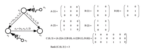
Each temporal edge e ∈ E represents a quadruple tuple e = {v_i, v_j, a_ij, t}, where v_i is the start node, v_j is the end node, and a_ij is the weight of edge e at time t [16]. If , then the temporal network can be shown in a discrete form of times [17]. At any given time t ∈ T, a temporal network can be extracted as a discrete snapshot graph G_t = (V, E_t), where E_t(u, v, t) ∈ E represents the set of edges active at time t. The sequence of these snapshot graphs captures the temporal evolution of the network [18]. The dynamics of a temporal network from a start time (t_s) to a desired time (t_d) can be displayed using graph snapshots. e.g., in Figure 1, a temporal network is shown from the t_s = 1 to t_d = 3.

Details are in the caption following the image — **Figure 1**
Open in figure viewer PowerPoint

A discrete temporal network including 5 nodes from start time t_s = 1 to desired time t_d = 3.

The dynamics of temporal networks, where connections between nodes evolve over time, can be effectively modeled using time-dependent linear discrete systems. These systems provide a mathematical framework to capture the time-varying nature of interactions, allowing for the analysis of how network structure influences dynamic processes such as information diffusion, synchronization, and epidemic spreading [19]. By representing the network’s adjacency matrix as a time-varying function, the model accounts for changes in connectivity patterns, enabling the study of both continuous and abrupt topological transitions. This approach is particularly useful in scenarios where the network’s evolution is driven by external factors or internal dynamics, offering insights into the stability, controllability, and performance of time-evolving networks. Linear discrete systems with time-dependent coefficients naturally extend classical network models to temporal settings, where the states of each node at a given time step depends linearly on its previous state and its neighbors’ states, weighted by the current network structure. Such models can incorporate periodic, stochastic, or arbitrary time variations in the network topology, making them adaptable to a wide range of applications, from social networks to biological systems. The analysis of these systems often involves tools from control theory, matrix algebra, and dynamical systems, allowing researchers to characterize transient and asymptotic behaviors. Additionally, this framework facilitates the study of how temporal correlations in link activations impact collective dynamics, providing a deeper understanding of the interplay between structure and dynamics in time-varying networks.

Moreover, the use of time-dependent linear systems enables the exploration of controllability and observability in temporal networks, addressing questions about how external inputs can steer the network toward desired states or how the system’s internal states can be inferred from limited observations. By leveraging concepts such as reachability and Gramian matrices adapted to discrete-time varying systems, it becomes possible to identify critical nodes and time windows that significantly influence the network’s behavior. This modeling paradigm not only bridges the gap between static network analysis and more realistic time-aware representations but also opens new avenues for optimizing interventions in dynamic networks, such as targeted vaccinations or strategic information dissemination. Thus, time-dependent linear discrete systems offer a versatile and powerful approach to understanding and harnessing the dynamics of temporal networks.

The dynamic equation of temporal networks is as follows (1) [20]:

()

where X(t): the state of the network nodes,

: the state vector at next time.

By expanding (1), the structural control matrix is obtained as (2)

()

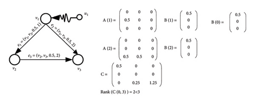
In this case, the network reaches fully controllability if rank(C(t_s, t_d)) = N. Figure 2 shows a temporal network i.e., completely controllable by the proper selection of control nodes. In Figure 2(a), the number of non-zero columns of matrix C is equal to 3. Therefore, the rank of matrix C is equal to 3. In the same way, In Figure 2(b), the rank of matrix C is equal to 2.

A temporal network becoming uncontrollable due to internal and external attacks refers to a scenario where strategic disruptions or failures prevent the network from being guided to a desired state, despite interventions [21]. Internal Attacks: These disruptions originate within the network itself. They can result from malicious activities by insiders, software bugs, hardware failures, or other internal issues that lead to the failure of nodes or edges [22]. External Attacks: These are caused by external entities or influences, such as cyber-attacks, environmental events, or targeted interventions by adversaries [23]. External attacks can disrupt the functionality of nodes or edges, affecting the network’s overall stability and performance. When a temporal network is subjected to internal and external attacks, its controllability can be significantly impaired. The attacks may target critical nodes and edges, which are essential for maintaining the ability to control the network. As a result, the network may become uncontrollable, meaning it is no longer possible to guide it to a desired state through any feasible set of interventions. This scenario has profound implications for the security and resilience of vital systems [24]. Imagine a communication network where nodes represent devices, and edges represent communication links active at specific times. An internal attack might involve compromised devices spreading misinformation, while an external attack might be a denial-of-service (DoS) attack disrupting communication links or intelligent attacks which are a type of deliberate attack that is done intelligently [25]. If critical control nodes and links are disrupted, the network might become uncontrollable, meaning we can no longer ensure that messages reach their intended recipients regardless of the interventions attempted [26].

In modern control systems, maintaining controllability is a critical aspect of ensuring the stability and performance of dynamic processes. However, these systems are increasingly vulnerable to various types of attacks that can disrupt their controllability, leading to severe consequences in industrial, automotive, and cyber-physical applications. Attacks on controllability processes can take multiple forms, including false data injection, DoS attacks, and stealthy deception attacks, each designed to manipulate or disable the system’s ability to regulate its states effectively. Such malicious interventions can compromise safety, efficiency, and reliability, making the study of attack detection and mitigation strategies essential for secure control system design. One of the most concerning aspects of these attacks is their ability to remain undetected while gradually degrading system performance. For instance, false data injection attacks can alter sensor readings or control inputs, misleading the controller into taking incorrect actions without triggering immediate alarms. Similarly, DoS attacks disrupt communication channels between sensors, actuators, and controllers, preventing timely updates and leading to loss of controllability. More sophisticated attacks, such as replay or covert attacks, exploit system vulnerabilities by replaying past data or carefully designed signals to evade traditional detection mechanisms. These threats highlight the need for robust security frameworks that integrate resilience into the controllability analysis of dynamic systems. The impact of attacks on controllability extends beyond immediate operational disruptions, potentially causing cascading failures in interconnected systems. In critical infrastructure, such as power grids or transportation networks, a loss of controllability due to cyberattacks can result in widespread outages or safety hazards. Researchers have thus focused on developing resilient control strategies, including attack identification, adaptive control reconfiguration, and secure communication protocols, to preserve controllability under adversarial conditions. By understanding the mechanisms through which attacks impair controllability, engineers and cybersecurity experts can design more robust systems capable of withstanding malicious interference while maintaining desired performance and safety standards.

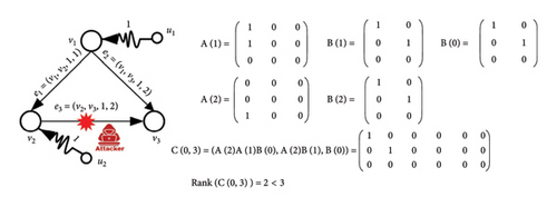
For example, in Figure 3, the e(v₂, v₃, 1, 2) is attacked by the attacker and removed at time t_a = 2. As a result, by calculating the rank of the control matrix C, it is determined that the network is out of the fully controllable state.

One promising approach to tackle this issue involves leveraging advanced techniques in network embedding (NE) and link prediction [27]. NE has emerged as a powerful tool for analyzing the controllability of temporal networks, offering a compact and meaningful representation of network dynamics that captures both structural and temporal features. By mapping nodes into a low-dimensional vector space, NE techniques enable the identification of critical nodes and edges that influence the system’s controllability, while preserving the inherent temporal dependencies and topological properties. These methods facilitate the efficient computation of control strategies by reducing the complexity of high-dimensional temporal networks, thereby enhancing our ability to predict and manipulate network behavior over time. Moreover, embedding-based approaches provide insights into the interplay between network evolution and controllability, allowing for the design of robust control frameworks that adapt to dynamic changes. As a result, NE serves as a bridge between traditional control theory and modern network science, offering scalable solutions for controlling complex temporal systems in fields such as neuroscience, transportation, and social networks. NE is a method that transforms high-dimensional network data into a lower-dimensional space, preserving the essential structural information [28]. This transformation facilitates easier manipulation and analysis of the network’s properties. On the other hand, link prediction aims to forecast missing or future connections within the network, enabling a proactive approach to maintaining and restoring network structure and controllability [29]. By integrating NE with link prediction, we can develop a robust framework for monitoring and recovering the controllability of temporal networks. NE aids in capturing the evolving patterns and structural nuances of the network over time [30]. This embedded representation, when coupled with sophisticated link prediction algorithms, allows us to predict and reinforce critical connections that are essential for network controllability [31]. The process begins with embedding the temporal network into a continuous vector space where the temporal dynamics are preserved. This embedded representation provides a more tractable form for analyzing network properties and predicting future links. Using link prediction models, we can identify potential new links or recover lost links that are crucial for maintaining controllability [32]. By strategically adding these predicted links, we can restore the network’s ability to be controlled from any initial state to any desired state, thus recovering its completely controllability. This approach not only enhances our capability to manage temporal networks effectively but also opens new avenues for applying machine learning and data-driven techniques in network science [33]. The synergy between NE and link prediction offers a powerful toolset for ensuring the robustness and functionality of dynamic networks across various domains, from communication and transportation systems to social and biological networks [34]. By maintaining the controllability of these networks, we can ensure their optimal performance and resilience in the face of continual change. Temporal NE provides a sophisticated framework for analyzing and understanding the complex dynamics of temporal networks [35]. Embedding nodes technique enables effective analysis and prediction of network behaviors [36]. Whether it is for link prediction, anomaly detection, or understanding the evolution of communities, temporal NE offers a powerful tool for researchers and practitioners dealing with dynamic and evolving networks.

Long Short-Term Memory (LSTM) addresses these challenges by leveraging their gated architecture, which selectively retains and forgets information, enabling effective learning of temporal patterns and robust prediction of network states. By integrating LSTM-based models into control frameworks, researchers can enhance the ability to steer temporal networks toward desired states, even in the presence of complex, nonlinear dynamics. This approach has significant implications for applications such as power grids, transportation systems, and biological networks, where adaptive and predictive control is essential for stability and performance. The combination of LSTMs and temporal network controllability thus offers a promising direction for advancing the understanding and optimization of time-dependent complex systems.

So far, methods have been proposed to restore controllability in temporal networks, generally after an error occurs in the controllability process of the network, by optimally adding nodes and edges, it has been tried to return the network to a completely controllable state. In this paper, using NE and link prediction, a novel recovery controllability method is proposed to restore the controllability of temporal networks by predicting the links under attack and embedding suitable nodes in the network.

Traditional temporal network analyses often treat each timestep independently, overlooking stable higher-order relationships between nodes. NE methods (e.g., Node2Vec, DeepWalk) address this by mapping nodes to a low-dimensional space while preserving structural properties such as community membership, centrality, and multihop connectivity. These embeddings provide a time-invariant backbone in temporal networks. While embeddings capture static topology, temporal networks require explicit modeling of evolving interactions. LSTM networks were selected over alternatives (e.g., RNNs, TCNs) due to their ability to handle irregular time intervals through adaptive gating mechanisms and, learn long-range dependencies across timesteps (critical for controllability trajectories), mitigate vanishing gradients in deep sequences.

The most important achievements of this article are:

•
Investigating the effects of various attacks on subordinate control processes in temporal networks.
•
Proposing a new method to recovery controllability based on the prediction of attack-prone links.
•
Using NE to reduce network dimensions in order to run controllable processes in massive networks.
•
Presenting the proposed recovery controllability method against intelligent and DoS attacks.

2. Related Works

Network controllability is a core principle in network science, enabling systems to transition from an initial state to a target state through controlled inputs. In temporal networks, where connections change dynamically, maintaining robust controllability is difficult because of shifting topologies. Recent progress combines temporal link prediction and NE techniques to improve controllability resilience. This section summarizes major contributions in the field.

Following the development of complex network controllability, researchers have explored recovery strategies to address disruptions caused by errors or attacks. Early work focused on static networks. For instance, Chen et al. analyzed how random and cascading failures impact controllability in static networks [37]. Ding et al. introduced algorithms to restore structural controllability in such networks by strategically adding links [38]. Zhang et al. modified maximum matching algorithms to recover controllability through the addition of control nodes [39, 40].

As temporal networks gained prominence for their real-world applicability, controllability methods adapted to dynamic environments. Subsequent research prioritized recovery strategies for temporal networks. Ding et al. developed algorithms to regain controllability by inserting new links, aligning with a layered structural controllability framework [41]. Feng and Tesi addressed controllability restoration after DoS attacks, proposing a link-strengthening approach to mitigate damage [42]. Saif et al. tackled delays induced by DoS attacks, introducing methods to safeguard controllability processes in temporal networks [24].

Robust controllability in temporal networks benefits from temporal link prediction and NE, enabling adaptive control strategies. Recent works highlight the synergy between these methods, but further advancements are needed to address scalability and uncertainty. Future integration with deep learning and causal modeling may unlock new possibilities for dynamic network control. The conventional controllability recovery algorithms restore the network after failures and attacks. If it can be prevented before the failures occur in the network, the controllable processes in the network will never be disturbed. Therefore, one of the important techniques in preventing attacks and failures in the network is link prediction. Using a convolutional neural network (CNN), Lou et al. have proposed a method that uses a neural network to identify the links that are becoming defective [43]. On the other hand, the most important challenge for controllability recovery algorithms in complex temporal networks is the large volume of data in real-world temporal networks. Currently, there are networks with a very high data volume that if the algorithms described above are used, their processing will take a long time or the recovery processes will be disrupted. One of the important techniques to speed up network algorithms is to reduce network dimensions by using NE [44]. Ma et al. have proposed NE for temporal networks [30].

In this paper, a new controllability recovery method is proposed, which reduces the dimensions of the network by using NE and then prevents disruptions in controllability processes by using link prediction based on temporal similarity.

In Table 1, the most important differences of the proposed method compared to other conventional recovery controllability methods are highlighted.

Table 1. Different methods of repairing the controllability compared to the proposed method.

Reference	Network type	Network attack	Model	Pruning process
[37]	Static	Random attacks	—	—
[38]	Static	Not investigated	—	—
[37]	Static	Not investigated	—	—
[38]	Static	Not investigated	—	—
[39]	Temporal	Degree attack	Layer model	—
[42]	Temporal	Not investigated	Layer model	—
[24]	Temporal	DoS attack	Layer model	Network embedding
[43]	Temporal	Centrality attack	Link Prediction/CNN	—
Proposed method	Temporal	Intelligent attacks DoS attack	Link Prediction/LSTM	Network embedding

3. The Proposed Recovery Controllability Method

Fully controllability in a network ensures that with a suitable choice of control inputs applied to a subset of nodes, known as driver nodes, the entire network can be driven to any target state. However, due to the dynamic nature of temporal networks, changes in the network structure can lead to periods where the network is no longer completely controllable. Identifying these periods of lost controllability is vital for effective network management and intervention. The process involves modeling the temporal network as a sequence of time-dependent adjacency matrices, identifying the necessary driver nodes, constructing the controllability matrix at each time step, and computing its rank. A drop in the rank below the total number of nodes in the network signals a loss of completely controllability. This method provides a systematic approach to ensure that interventions can be made promptly to restore or maintain control over the network.

In this paper, a measure is proposed to detect when the network is out of completely controllability, which indicates the degree of controllability of the network at any moment. The degree of controllability obtained from (3) has a value between 0 and 1. If the degree is 1, it means that the network can be completely controlled by control nodes. If the controllability degree value is less than 1, it indicates that the control nodes have included a smaller number of network nodes under their control coverage.

()

When the network is in completely controllability mode and the network is attacked, the most important criterion to determine that the attacked network is out of completely controllability mode is the doc criterion. Networks after the attack, their DoC value will be less than 1. The stronger the attack, the more the DoC value tends to zero.

Temporal NE is a powerful technique designed to address this need by representing the evolving network in a continuous vector space while preserving its temporal and structural characteristics. Temporal NEs can predict future or missing links in the network by leveraging the learned temporal dynamics and node interactions.

Definition 1. Temporal NE: Given a temporal network G = (V, E, T) and the corresponding time-stamped adjacency matrix A, temporal NE aims to learn a mapping function f : vi ⟶ yi ∈ R^d. The objective of the function is to make the similarity between y_i and y_i preserve the temporal proximity between v_i and v_j.

Definition 2. Temporal Node Embedding: Let d ≥ 1 be the dimensionality of the node embeddings. A node embedding function f is a map f : V⟶V^′ ∈ R^d maps each node v ∈ V to a real-valued feature vector in v^′ ∈ R^d.

Definition 3. Temporal Link Prediction: Given a series of snapshots {G_t − N, G_t − N + 1, …, G_t} of an evolving graph G_t = 〈V, E_t〉 in which each e = (u, v) ∈ E_t represents a link between u and v that took place at a particular time t. We seek to predict the most likely link state in the next time step G_t+1. The temporal link prediction also called a periodic link prediction when N ≫ 0.

In this paper, a novel framework is proposed for NE the complex temporal network and predicting the broken links. In Recovery Controllability using the Temporal Embedding Network (RCTE) Framework, by embedding the network and reducing the dimensions of the time network, the speed of the controllability recovery process should be increased, and then the network controllability is restored by predicting the links that are failing. NE excels in preserving persistent topological features by encoding nodes into low-dimensional vectors that capture structural properties (e.g., centrality, community structure), enabling robust identification of driver nodes invariant to temporal noise. Meanwhile, LSTMs model complex temporal dynamics by learning long-range dependencies and adapting to irregular time intervals, which is critical for predicting evolving controllability requirements. Together, their integration offers synergistic advantages: embeddings provide a stable structural prior to guide LSTM predictions, while LSTMs dynamically refine these representations to adapt to time-varying interactions. This hybrid approach ensures robust controllability, balancing topological stability with temporal adaptability and, outperforms methods relying solely on static or temporal information, as demonstrated by reduced control energy and higher prediction accuracy in experiments.

The combined framework effectively leverages the complementary strengths of both approaches to achieve superior temporal network controllability. NEs provide topology-aware initialization for LSTMs, offering stable structural priors that significantly reduce overfitting to transient temporal patterns. Simultaneously, the LSTM component dynamically refines these embeddings by incorporating temporal dependencies across network states, enabling adaptive controllability strategies that evolve with the network. Crucially, the static nature of the underlying embeddings serves as a powerful regularizer, constraining the LSTM’s learning process and preventing overfitting to noisy short-term fluctuations. This dual mechanism ensures robust performance by maintaining structural consistency while accommodating necessary temporal adaptations, ultimately yielding more reliable controllability outcomes than either method could achieve independently.

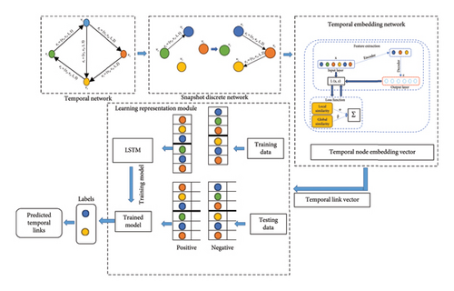
The different components of the RCTE framework are shown in Figure 4. As seen in Figure 4, a temporal network is transformed into snapshots of static networks at discrete times. Then, in the temporal NE process, the dimensions of the temporal network are reduced and, temporal node embedding vectors are formed. After that, in the learning representation module, a learning model is built using the LSTM neural network, which can be used to predict the failing links.

3.1. Temporal Embedding Network and Feature Extraction

The design often incorporates advanced techniques like attention mechanisms or transformers to enhance performance, making it highly effective for sequence-to-sequence and generative tasks. This architecture has become a cornerstone in modern AI systems due to its flexibility, scalability, and ability to generalize across diverse domains. In the RCTE framework, a decoder-encoder is designed based on deep neural networks to recognize the information about the structure and the network characteristics. In this method, a powerful threshold is presented to evaluate the loss rate of the encoder-decoder by combining local and global characteristics. Therefore, the efficiency of the link prediction algorithm has increased with the loss function improvement in the encoder-decoder. Figure 5 shows the steps of the temporal NE. In the process of temporal embedding network, the input layer is reduced to smaller dimensions, and then the NE is done using the loss function L and based on two criteria of local and global similarity.

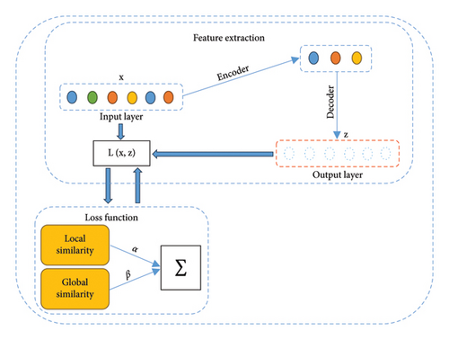
Extracting the feature is the most important part of the RCTE framework, which is done by an encoder-decoder. Encoder-decoders play an essential role in unsupervised learning and deep networks. The purpose of using encoders is to represent data in a way that to be used in classification. The best advantage of encoder-decoders is the automatic selection of features. As can be seen in Figure 6, the encoder is a neural network that receives a set of data without labels encrypts them and, tries to represent the inputs at the output so that they have the least possible difference with the input value. In encoding, the input data is mapped to the attribute space, and in decoding, space is converted from the attribute space back to its original state. The main part of an encryption-decoder is the intermediate hidden layer that is used as the extracted property for categorization.

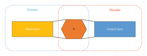
Autoencoders are a type of neural network designed to learn efficient representations of input data by compressing it into a lower-dimensional latent space and then reconstructing it back to the original form. The primary objective of an autoencoder is to minimize the reconstruction loss, which measures the difference between the input data and its reconstructed output. By doing so, the model learns to capture the most salient features of the data while discarding noise or irrelevant details. This process involves an encoder that maps the input to a compressed representation and a decoder that attempts to reconstruct the input from this representation. The quality of the reconstruction depends on the autoencoder’s ability to balance compression with fidelity, ensuring that the latent space retains enough information to reproduce the input accurately. Minimizing reconstruction loss is crucial for applications such as dimensionality reduction, denoising, and anomaly detection, where preserving essential data characteristics is key.

The encoder with f_θ, and the data set with X_i, the (4) is established.

()

The vector h is the calculated property of x at time t. The decryption section is a function that displays it with and according to the (5) mapping maps of the space characteristic of latent features or the latent space makes its way into the entrance space.

()

3.2. Loss Function

Using global information in loss calculation leads to high accuracy, but it takes a lot of time to be calculated. On the other hand, actions based on local information are generally faster but provide less accuracy. Because the network type is large-scale, irregular, and heterogeneous real-world networks, both local and global structures are important. In the RCTE framework, by combining local and global features, the accuracy of the loss function has improved.

Node degree centrality is a fundamental concept in network analysis, measuring the importance of a node based on the number of connections it has to other nodes [45]. In static networks, this is a straightforward count of edges, but in temporal networks, where connections can change over time, the concept becomes more complex and dynamic. Degree centrality in temporal networks can be measured in several ways. One approach is to consider the cumulative degree over the entire observation period, summing the instances when a node is connected to others. Another approach is to analyze snapshots of the network at different time intervals, calculating the degree of centrality for each snapshot and possibly aggregating these values to understand trends and patterns. Temporal degree centrality is a measure of node importance in a temporal network, reflecting how the connectivity of a node changes over time. The temporal degree centrality C_D(v, T) of a node v ∈ V over the time T can be defined in multiple ways. One common approach is the cumulative temporal degree centrality, which sums the instances of connections for the node over the entire observation period. This can be expressed as (6)

()

where d(v, t) represents the degree of node v at a specific time t, that is, the number of edges incident to v that are active at time t and N is the number of network nodes.

Based on (6), the local similarity is obtained as (7)

()

where

is the set of neighbors of node v_i.

To ensure a fair comparison, we might normalize the degree of centrality values at each time step before aggregation. This can be done by dividing each degree of centrality by the maximum degree centrality observed at that time. The normalized temporal degree centrality vectors of neighbors w at time t are abstained as (8)

()

Finally, the local similarity measure now becomes as (9)

()

where • X.Y is the dot product of the two vectors. • ‖X‖ is the magnitude (Euclidean Norm) of the vector X.

To compute the global similarity of nodes in a temporal network, you need to consider the entire temporal structure of the network, including how nodes interact over time. Global similarity involves understanding how similar the nodes are based on their roles and connections in the network across all time steps. Temporal closeness centrality is one of the most important global structural criteria in a temporal network. Calculate the temporal closeness centrality for each node over all relevant periods. This involves finding the shortest temporal paths that respect the chronological order of interactions. To calculate the global similarity of nodes in temporal networks using temporal closeness centrality, you need to adapt the concept of closeness centrality to the temporal context and then measure similarity based on these centrality values over the entire network and across the entire period. To calculate the global similarity to the sound, the following has been done:

•
Compute the temporal shortest path from each node to every other node at each time step.
•
Calculate the temporal closeness centrality by summing up the temporal distances and using the reciprocal for centrality.
•
For each node, create a vector where each element is the temporal closeness centrality value at a specific time step.
•
Use cosine similarity (or another similarity measure) to compute the similarity between the vectors of all pairs of nodes.

A path in a temporal network that respects the chronological order of interactions. A temporal shortest path from node u to node v at time t is the quickest path that respects the order of interactions. Temporal closeness centrality measures how close a node is to all other nodes over time. For a node c ∈ V at time t ∈ T, its temporal closeness centrality C_C(v, t) can be defined as the reciprocal of the sum of shortest path lengths from v to all other nodes at time t. It is abstained as (10)

()

where d_s(v, u, t) is the temporal shortest distance from v to u at time t.

To ensure comparability across different time steps, normalize the temporal closeness centrality values. For a node v at time t, the normalized temporal closeness centrality

can be obtained by dividing the temporal closeness centrality by the maximum temporal closeness centrality observed at that time as (11)

()

For each node u ∈ V, construct the temporal closeness centrality vector of its neighbors over all time steps. Let N(u) denote the set of neighbors of u. The temporal closeness centrality vector

at time t is defined as (12)

()

Aggregate these vectors over the entire period T is obtained as (13)

()

To determine the temporal similarity between two nodes u and v, compute the cosine similarity between their aggregated and normalized temporal closeness centrality vectors of their neighbors. It’s abstained as (14)

()

where • X.Y is the dot product of the two vectors. • ‖X‖ is the magnitude (Euclidean Norm) of the vector X.

The loss function is obtained based on local and global temporal similarity. The local loss function is obtained as (15):

()

where h_i indicates the node feature vector and Sim_local(i, j, T) represents the local Similarity network at T.

The global loss function is obtained as (16)

()

To optimize the loss function, a combination of local and global loss function is used, which is obtained as (17)

()

The α and β are hyperparameters that are responsible for controlling the balance between the two global similarity and local similarity thresholds. The α hyperparameter determines the effectiveness of the local criterion. If α = 0, the predictive function is performed only through the global threshold. The β hyperparameter indicates the effect of the global standard effect on the prediction operation.

3.3. Learning Representation Module

Representation learning involves discovering the best way to represent data to make it easier for machine learning algorithms to perform tasks like classification, regression, clustering, and more. LSTM networks, a specialized variant of recurrent neural networks (RNNs), are particularly well-suited for handling sequential data due to their ability to capture long-term dependencies and mitigate the vanishing gradient problem. In the context of recovery controllability, LSTMs can model the evolving structure of temporal networks, predict potential failure points, and optimize control strategies to restore system functionality efficiently. By leveraging their memory cells and gating mechanisms, LSTMs can retain and utilize historical network states to inform real-time decision-making, making them ideal for dynamic control scenarios. This capability is especially valuable in scenarios where the network topology changes unpredictably, such as in disaster response or power grid recovery. The integration of LSTM networks into recovery controllability frameworks offers a data-driven alternative to traditional model-based control methods. Unlike static approaches, LSTMs can adapt to the temporal evolution of network dynamics, enabling more resilient and responsive control strategies. For instance, in a transportation network disrupted by an unexpected event, an LSTM-based controller could analyze past traffic patterns, predict congestion propagation, and recommend optimal rerouting strategies to restore normal operations. Furthermore, the ability of LSTMs to process high-dimensional, nonlinear temporal data makes them suitable for complex networks where analytical solutions are intractable. The application of LSTM neural networks in recovery controllability of temporal networks represents a promising intersection of machine learning and control theory. By harnessing the predictive and adaptive capabilities of LSTMs, researchers and practitioners can develop more robust and scalable solutions for managing dynamic networks under uncertainty. Future advancements in this area could further enhance the autonomy and efficiency of control systems, paving the way for smarter and more resilient infrastructure in an increasingly interconnected world.

In this paper, the LSTM network is used to represent learning. The formulation of an LSTM network involves defining the mathematical operations that govern the flow of information through its architecture. An LSTM cell is designed to maintain long-term dependencies by carefully regulating the information that flows through its internal state using gates.

The forget gate decides which information to discard from the previous cell state. It takes the previous hidden state (h_t−1) and the current input (x_t), and applies a sigmoid activation function (18):

()

The input gate determines which new information to add to the cell state. The candidate cell state (

) is created using a tanh activation function (19) and (20):

()

The cell state is updated by combining the previous cell state, scaled by the forget gate, and the candidate cell state, scaled by the input gate (21):

()

The output gate decides what the next hidden state should be. It uses the updated cell state and applies a tanh activation function to it, combined with the output gate (22) and (23):

()

where • W_f, W_i, W_C, W_o are weight matrices. • b_f, b_i, b_C, b_o are bias vectors for the respective gates. • σ(x) = 1/(1 + e^−x).

4. Simulations and Evaluation the Proposed Methods

The proposed controllability restoration method based on the RCTE framework enables controllability restoration processes to be performed with high speed and optimal accuracy. To evaluate the performance of the proposed recovery method, the method has been simulated in the Python environment and several tests have been performed to check its performance compared to other conventional methods.

To evaluate the effectiveness of the proposed controllability recovery method, the proposed method has been implemented on four real-world datasets related to temporal networks [46]. The selected datasets have a high diversity in the internal dynamics of the network. The most important features of the selected datasets can be seen in Table 1. In Table 2, assortativity means the tendency of nodes to connect to similar or dissimilar nodes based on the specific characteristics of nodes.

Table 2. Dataset properties.

	N	L	Density L/N(N − 1)	d_max/d_min/d_avg	Average clustering coefficient	Assortativity
Email network	33.7 K	180.8 K	0.000318501	1.4K/1/10	0.50919	−0.116499
Collaboration network	28.1 K	4.6 M	0.0116494	11.1K/1/327	1.53173	0.149852
Facebook friendship	63.7 K	1.3 M	0.000625128	1.8K/1/39	0.211799	0.163713
Wikibooks	8.4 K	162 K	0.00461677	11.3K/1/38	2.12468	0.0538031

As mentioned earlier, controllable processes in temporal networks face internal and external attacks and failures. Internal attacks are the random failures that occur in the network. These failures include disconnections or routers, and failures of servers and workstations. Intelligent attacks are based on the information obtained from different characteristics of nodes and edges of the network. In this paper, four common types of attacks are selected. These attacks are defined based on scenarios. Temporal Random attacks represent random failures in the network. A temporal degree centrality attack is a type of intelligent attack that occurs based on the local information of the network, which is the temporal degree of the nodes. A temporal closeness centrality attack is a type of intelligent attack that occurs based on the temporal closeness centrality of nodes and uses global network information. DoS attacks do not occur based on the characteristics of the network components, but by creating disturbances on the network links, they cause the links to be interrupted. In general, the temporal degree centrality attack occurs on both nodes and links, the temporal closeness centrality attack occurs only on nodes, and the DoS attack occurs only on links.

Attack scenarios are defined here for random and intelligent failures. The defined attack scenarios are:

•
Temporal Random Attack Scenario (TRA): Links and nodes with removal rate are randomly removed from the network in time interval T = [t₁, t₂].
•
Temporal Degree Centrality Attack Scenario (TDA): Nodes are deleted in the order of their temporal degree centrality in descending order with the rate in the time interval T = [t₁, t₂].
•
Temporal Closeness Centrality Attack Scenario (TCA): Nodes are deleted in the order of their temporal closeness centrality in descending order with the rate in the time interval T = [t₁, t₂].
•
Temporal DoS Attack Scenario (TDoS): The links are deleted based on the distribution function and DoS attack parameters with the attack rate in the time interval T = [t₁, t₂].

The attack rate means the probability of an attack at any moment, which is equal to the ratio of the number of links/nodes removed to the total number of links/nodes in the network.

In the conducted attack experiments, the attack rate is considered. The parameters of DoS attacks are set as distributed function: Poisson process, mean service time = 3 s, background traffic load: 0.6, sampling rate = 50 samples/s, measurements packets from an attacker = 750, stochastic delay jitter = 7. The duration of the simulation was 15 min, and the results of the experiments based on random processes were reported as an average of 50 executions.

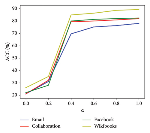
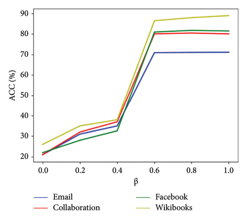
In order to determine the values of the α and β parameters, a sensitivity analysis of the hyperparameters α (global similarity weight) and β (local similarity weight) is performed and, the impact of global/local similarity weights (α, β) on model performance is evaluated. In the experiment, the proposed method is performed on datasets based on random attacks. In the first experiment, the value of parameter α ∈ [0, 1] is considered constant and the value of β is variable. In the second experiment, the value of β ∈ [0, 1] is considered constant and the value of α is variable. Figure 7 shows that if the values of α = 0.4 and β = 0.6 are, the performance of the learning model based on the ACC evaluation parameter is stable.

Performance evaluation in deep learning involves assessing how well a model performs on a given task, typically by using various metrics and techniques. Accuracy is a performance metric for classification models that measures the proportion of correctly classified instances among the total instances. It is a widely used metric for assessing the overall effectiveness of a classifier, particularly when the class distribution is balanced. Accuracy is the ratio of the sum of true positives and true negatives to the total number of instances. It reflects how often the classifier is correct over the entire dataset. Given a classification problem with n instances:

()

where • TP: True Positives. • TN: True Negatives. • FP: False Positives. • FN: False Negatives.

Accuracy is most useful when the classes are roughly equal in size. In cases where there is a significant class imbalance, accuracy might be misleading. For imbalanced datasets, other metrics like the F1 Score might provide more insight into the model’s performance. The F-Measure, or F1 Score, is a performance metric for classification models that considers both precision and recall to provide a single score that balances the two. It is especially useful in situations where the class distribution is imbalanced. Given a classification problem, the F1 Score is the harmonic mean of Precision (P) and Recall (R):

()

where

()

All models are trained using 75% of the data and then tested and checked using the remaining 25% of the data.

In Table 3 the effectiveness of the learning model in the RCTE method is compared to the controllability recovery method based on the NE [24] and CNN neural network [43] different attack strategies with different attack rates on datasets. The evaluation results demonstrate that the proposed RCTE method consistently outperforms both CNN and GNN-based controllability recovery methods across various attack strategies and datasets. This trend persists even at higher attack rates (e.g., 0.8), where RCTE maintains superior performance over CNN and NE. Similar improvements are observed in other datasets, such as Wikibooks, where RCTE achieves exceptional ACC (up to 0.989) and F1 scores (up to 0.970), significantly surpassing CNN and NE. The robustness of RCTE is particularly evident in adversarial scenarios, highlighting its enhanced capability to recover network controllability under diverse attack conditions. These results suggest that RCTE’s innovative approach effectively mitigates the limitations of traditional neural network-based methods, offering a more reliable solution for maintaining network integrity. On the other hand, the results show that, in general, the efficiency of the learning model increases with the increase in the attack rate, but in the proposed method, the efficiency of the learning model has increased with a greater slope, which indicates the high efficiency of proposed learning model with an increase in the attack rate. Finally, in datasets where the intensity of network dynamics and its changes are high, the accuracy of the learning model in the proposed method is much higher compared to the CNN and NE methods (in intelligent and DoS attacks is more than 95%).

Table 3. Evaluation learning model in the RCTE method compared to the controllability recovery method based on the CNN and GNN neural network in different attack strategies.

Model features			NE				CNN				RCTE (our)
Dataset		Attacks measure	TRA	TDA	TCA	TDoS	TRA	TDA	TCA	TDoS	TRA	TDA	TCA	TDoS
Email network	0.2	ACC	0.675	0.681	0.692	0.675	0.683	0.682	0.695	0.685	0.695	0.708	0.718	0.704
	0.2	F₁	0.661	0.675	0.689	0.671	0.681	0.685	0.699	0.680	0.692	0.701	0.712	0.700
	0.4	ACC	0.681	0.690	0.710	0.685	0.692	0.699	0.717	0.698	0.701	0.719	0.727	0.722
	0.4	F₁	0.673	0.691	0.690	0.682	0.698	0.702	0.722	0.700	0.709	0.730	0.738	0.728
	0.6	ACC	0.683	0.693	0.709	0.695	0.693	0.709	0.728	0.710	0.712	0.729	0.746	0.731
	0.6	F₁	0.680	0.695	0.708	0.690	0.686	0.713	0.731	0.721	0.710	0.742	0.758	0.748
	0.8	ACC	0.688	0.725	0.734	0.723	0.690	0.718	0.739	0.718	0.720	0.735	0.741	0.738
	0.8	F₁	0.689	0.701	0.712	0.709	0.701	0.725	0.721	0.725	0.711	0.752	0.763	0.741

Collaboration network	0.2	ACC	0.671	0.676	0.789	0.774	0.680	0.789	0.798	0.768	0.793	0.803	0.816	0.801
	0.2	F₁	0.658	0.669	0.786	0.772	0.689	0.781	0.795	0.781	0.791	0.800	0.810	0.799
	0.4	ACC	0.678	0.689	0.701	0.780	0.713	0.790	0.724	0.789	0.799	0.812	0.825	0.820
	0.4	F₁	0.669	0.687	0.784	0.779	0.745	0.799	0.748	0.795	0.801	0.828	0.836	0.826
	0.6	ACC	0.681	0.689	0.702	0.789	0.750	0.802	0.752	0.803	0.808	0.825	0.842	0.830
	0.6	F₁	0.679	0.692	0.701	0.785	0.745	0.808	0.763	0.813	0.805	0.839	0.854	0.843
	0.8	ACC	0.684	0.715	0.728	0.713	0.774	0.818	0.783	0.809	0.818	0.832	0.839	0.834
	0.8	F₁	0.685	0.698	0.702	0.702	0.740	0.823	0.801	0.812	0.801	0.849	0.859	0.839

Facebook friendship	0.2	ACC	0.779	0.787	0.796	0.779	0.783	0.795	0.801	0.789	0.799	0.819	0.822	0.818
	0.2	F₁	0.768	0.783	0.792	0.777	0.774	0.798	0.802	0.786	0.786	0.815	0.819	0.816
	0.4	ACC	0.786	0.794	0.813	0.789	0.789	0.802	0.814	0.795	0.812	0.829	0.834	0.824
	0.4	F₁	0.776	0.792	0.794	0.783	0.788	0.812	0.821	0.799	0.810	0.842	0.842	0.839
	0.6	ACC	0.788	0.796	0.815	0.798	0.795	0.816	0.825	0.805	0.819	0.836	0.845	0.838
	0.6	F₁	0.785	0.799	0.812	0.795	0.799	0.824	0.828	0.812	0.818	0.849	0.864	0.852
	0.8	ACC	0.795	0.729	0.838	0.826	0.803	0.827	0.831	0.811	0.823	0.842	0.846	0.841
	0.8	F₁	0.792	0.704	0.815	0.810	0.812	0.830	0.839	0.825	0.815	0.859	0.869	0.856

Wikibooks	0.2	ACC	0.785	0.804	0.810	0.809	0.793	0.814	0.823	0.818	0.838	0.869	0.892	0.872
	0.2	F₁	0.775	0.899	0.805	0.800	0.799	0.818	0.825	0.816	0.822	0.859	0.882	0.864
	0.4	ACC	0.792	0.812	0.818	0.819	0.805	0.824	0.832	0.824	0.842	0.875	0.895	0.875
	0.4	F₁	0.782	0.808	0.812	0.808	0.812	0.828	0.845	0.821	0.825	0.863	0.885	0.868
	0.6	ACC	0.798	0.823	0.823	0.828	0.818	0.835	0.841	0.835	0.885	0.892	0.898	0.895
	0.6	F₁	0.795	0.810	0.819	0.812	0.825	0.845	0.856	0.842	0.880	0.885	0.890	0.886
	0.8	ACC	0.804	0.835	0.842	0.832	0.856	0.849	0.879	0.891	0.932	0.962	0.989	0.969
	0.8	F₁	0.801	0.814	0.818	0.818	0.864	0.841	0.898	0.899	0.910	0.938	0.970	0.955

To investigate the destructive effects of different attacks on network controllability processes, attacks based on different scenarios have been carried out on datasets. In the attacks carried out, the rate of attacks is . As mentioned earlier, the DoC measure is proposed to determine the control coverage of the network by the control nodes. The smaller the network DoC, the more nodes are out of control. Figure 8 shows the D/N based on the attack rate (R). As can be seen in Figure 8, the number of control nodes (D) has increased with the increase in the attack rate. In general, the results demonstrate that the destructive effects of TCA and TDoS attacks were greater in crowded datasets than in other attacks. On the other hand, the TDA attack has been more destructive than other attacks in datasets with high dynamic intensity.

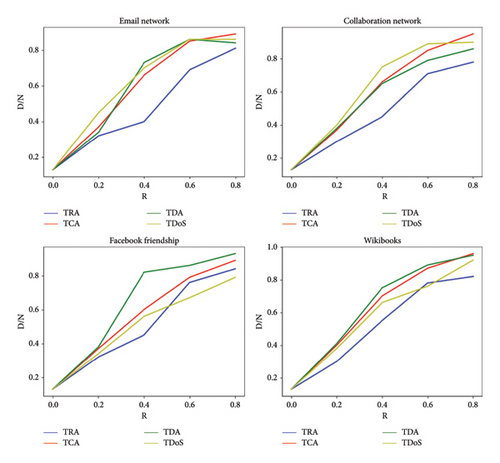
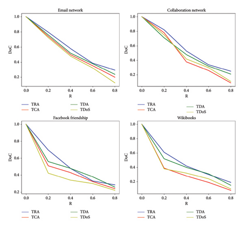
Figure 9 demonstrates the effects of attacks on network controllability. The results show that with the increase in the attack rate, the networks with a high gradient leave a state of completely controllability. The speed of leaving completely controllability in TCA and TDoS attacks is higher than other attacks.

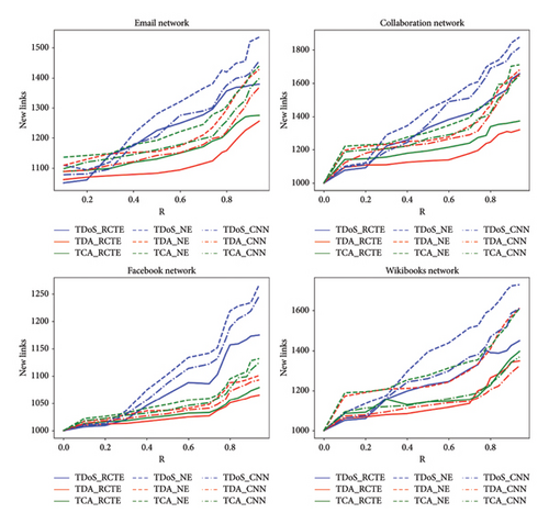
By implementing the proposed recovery method (RCTE) and comparing it with the CNN method, the number of new links added to the network to prevent disturbance in the control processes can be seen in Figure 10. In controllability recovery methods, the lower the number of new links added to the network, the better the performance of that method. The data reveals notable differences in the effectiveness of various methods in mitigating the impact of attacks on network links. The RCTE method consistently demonstrates superior performance across all attack types, as evidenced by the fewer new links added compared to the NE and CNN methods. This suggests that the RCTE approach is more robust in maintaining network stability under adversarial conditions. In contrast, the NE method tends to result in a higher number of new links, indicating a less efficient response to attacks. The CNN method falls between the RCTE and NE methods, showing moderate effectiveness but still requiring more link additions than the RCTE approach. When examining the impact of different attack types, RA attacks appear to be the most disruptive, as they generally necessitate the highest number of new links across all methods. DA and BA attacks, while still harmful, are comparatively less severe, with fewer links required for recovery. This pattern holds true regardless of the mitigation method used, reinforcing the notion that RA attacks are particularly challenging to counter. The consistency of this trend suggests that network defenses may need to prioritize strategies specifically tailored to resist RA attacks. The discussion underscores the importance of selecting appropriate mitigation techniques based on the attack type. The RCTE method emerges as the most efficient, but further research could explore whether its advantages hold under more varied or intense attack scenarios. Additionally, the relatively poor performance of the NE method raises questions about its suitability for dynamic or large-scale networks. The CNN method, while not as effective as RCTE, may offer a balance between complexity and performance, warranting further investigation into its optimization. Overall, the findings highlight the need for adaptive and attack-specific strategies to minimize network disruptions. The results demonstrate that in all datasets, the RCTE method performed better than the CNN method and repaired the network with fewer new links. The improvement has been higher in datasets with high dynamics. Also, the efficiency of the RCTE method in malicious TCA and TDoS attacks is significant.

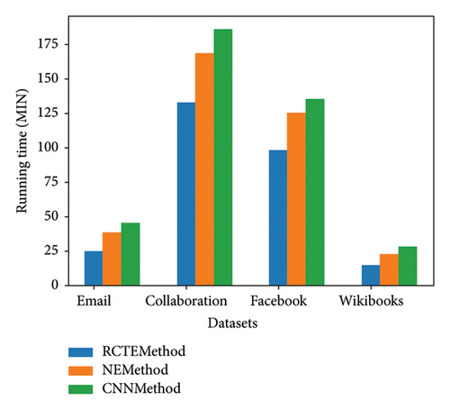
One of the efficiency criteria of recovery controllability methods is their execution speed. Considering that the speed of control processes in massive networks is low, the high recovery speed of control processes can play an important role in preventing the disruption of these types of processes. Figure 11 shows the execution time of different methods. The data highlights clear differences in computational efficiency among the three methods, with the RCTE method consistently demonstrating the fastest running times. This suggests that the RCTE approach is the most computationally efficient, requiring less time to execute compared to the NE and CNN methods. The NE method, while slower than RCTE, still outperforms the CNN method, which exhibits the longest running times. This trend indicates that the RCTE method may be better suited for real-time or time-sensitive applications where rapid processing is critical. The performance gap between the methods raises important considerations about the trade-offs between computational speed and other factors, such as accuracy or robustness. While the CNN method is the slowest, it may offer advantages in certain scenarios, such as handling complex or high-dimensional data, that justify its increased computational cost. Conversely, the efficiency of the RCTE method makes it an attractive option for systems where speed is prioritized, provided it meets other performance requirements. The NE method occupies a middle ground, potentially offering a balance between speed and functionality. These findings emphasize the importance of selecting a method based on the specific demands of the application. For tasks requiring rapid execution, the RCTE method is the most suitable, whereas the CNN method might be reserved for cases where its additional capabilities outweigh its slower performance. Further research could explore whether optimizations or hybrid approaches could improve the speed of the slower methods without compromising their effectiveness. Overall, the data underscores the need to align method selection with operational priorities, particularly in environments where computational efficiency is a key constraint.

5. Conclusion

In this paper, a new method to restore controllability in temporal networks is proposed. For this purpose, a new framework called RCTE has been proposed, in which the speed of recovery processes has been increased by reducing the dimensions of network data. In the framework of RCTE, by providing a learning model based on the LSTM neural network, links prone to failure have been identified to prevent disruptions in control processes. The experimental results demonstrate that the proposed RCTE method significantly outperforms existing CNN and NE-based approaches in recovering network controllability under various attack scenarios. Across multiple datasets and attack rates, RCTE consistently achieves higher accuracy, robustness, and efficiency, particularly in adversarial conditions where traditional methods struggle. Notably, RCTE maintains superior performance even at high attack intensities, requiring fewer new links to restore network stability compared to CNN and NE methods. This efficiency is especially pronounced in highly dynamic networks and against sophisticated attacks such as TCA and TDoS, where RCTE exhibits remarkable resilience. Additionally, RCTE excels in computational efficiency, executing recovery processes faster than both CNN and NE methods. This speed advantage makes it particularly suitable for real-time applications where rapid response is critical to maintaining network integrity. While CNN and NE methods may offer certain strengths in handling complex data structures, their slower performance and higher resource demands limit their effectiveness in time-sensitive scenarios. The findings suggest that RCTE strikes an optimal balance between speed, accuracy, and adaptability, making it a compelling solution for modern network controllability challenges. Future research could explore further optimizations of RCTE, such as hybrid approaches that integrate neural network strengths while preserving its computational efficiency. Additionally, testing RCTE under even more extreme attack conditions or in larger-scale networks could validate its scalability and robustness further. Overall, this study highlights RCTE as a highly effective and efficient method for controllability recovery, offering a reliable alternative to conventional neural network-based approaches in securing dynamic and adversarial network environments.

Disclosure

This work was sponsored in part by the Bidding Projects of Key Disciplines during the 14th Five—Year Plan Period of Xinjiang Normal University (Research on School Education for Strengthening the Sense of the Chinese Nation Community, 24XJKD0109) and, Xinjiang Teacher Education Research Center (Research on the Promoting Role of Progressive Teaching, Research and Training Integrated Activities on the Teaching and Research Abilities of Primary and Secondary School Mathematics Teachers, ZK2024W10).

Conflicts of Interest

The authors declare no conflicts of interest.

Funding

Open Research

Data Availability Statement

The data that support the findings of this study are available on request from the corresponding authors. The data are not publicly available due to privacy or ethical restrictions.

References

1 Zhang L., Marzuki A., Liao Z., Zhao K., Huang Z., and Chen W., Spatial and Temporal Evolution of Guangdong Tourism Economic Network Structure From the Perspective of Social Networks, Heliyon. (2023) 9, no. 8, https://doi.org/10.1016/j.heliyon.2023.e18570.
10.1016/j.heliyon.2023.e18570
Web of Science® Google Scholar
2 Salama M., Ezzeldin M., El-Dakhakhni W., and Tait M., Temporal Networks: A Review and Opportunities for Infrastructure Simulation, Sustainable and Resilient Infrastructure. (2022) 7, no. 1, 40–55, https://doi.org/10.1080/23789689.2019.1708175.
10.1080/23789689.2019.1708175
Web of Science® Google Scholar
3 Zhang Y., Xia Y., and Wang L., On the Reachability and Controllability of Temporal Continuous-Time Linear Networks: A Generic Analysis, Automatica. (2024) 167, https://doi.org/10.1016/j.automatica.2024.111741.
10.1016/j.automatica.2024.111741
Web of Science® Google Scholar
4 Wang R., Zhang Q., Zhang Y., Shi H., Nguyen K. T., and Zhou X., Unconventional Split Aptamers Cleaved at Functionally Essential Sites Preserve Biorecognition Capability, Analytical Chemistry. (2019) 91, no. 24, 15811–15817, https://doi.org/10.1021/acs.analchem.9b04115.
10.1021/acs.analchem.9b04115
CAS PubMed Web of Science® Google Scholar
5 Zhang H., Zou Q., Ju Y., Song C., and Chen D., Distance-based Support Vector Machine to Predict DNA N6-Methyladenine Modification, Current Bioinformatics. (2022) 17, no. 5, 473–482, https://doi.org/10.2174/1574893617666220404145517.
10.2174/1574893617666220404145517
CAS Web of Science® Google Scholar
6 Cao C., Wang J., Kwok D. et al., webTWAS: A Resource for Disease Candidate Susceptibility Genes Identified by Transcriptome-Wide Association Study, Nucleic Acids Research. (2022) 50, no. D1, D1123–D1130, https://doi.org/10.1093/nar/gkab957.
10.1093/nar/gkab957
CAS PubMed Web of Science® Google Scholar
7 Yang Y., Liu J., and Zhou X., A CRISPR-Based and Post-amplification Coupled SARS-CoV-2 Detection With a Portable Evanescent Wave Biosensor, Biosensors and Bioelectronics. (2021) 190, https://doi.org/10.1016/j.bios.2021.113418.
10.1016/j.bios.2021.113418
Web of Science® Google Scholar
8 Liu Y.-Y., Slotine J.-J., and Barabási A. L., Controllability of Complex Networks, Nature. (2011) 473, no. 7346, 167–173, https://doi.org/10.1038/nature10011, 2-s2.0-79955879494.
10.1038/nature10011
CAS PubMed Web of Science® Google Scholar
9 Arebi P., Fatemi A., and Ramezani R., Event Stream Controllability on Event-Based Complex Networks, Expert Systems with Applications. (2023) 213, https://doi.org/10.1016/j.eswa.2022.118886.
10.1016/j.eswa.2022.118886
Web of Science® Google Scholar
10 Xia K., Li Z., and Zhou X., Ultrasensitive Detection of a Variety of Analytical Targets Based on a Functionalized Low-Resistance AuNPs/β-Ni (OH) 2 Nanosheets/Ni Foam Sensing Platform, Advanced Functional Materials. (2019) 29, no. 39, https://doi.org/10.1002/adfm.201904922, 2-s2.0-85070062598.
10.1002/adfm.201904922
Google Scholar
11 Sun P., Kooij R. E., and Bouffanais R., Controllability of a Class of Swarm Signalling Networks, Journal of Complex Networks. (2022) 10, no. 6, https://doi.org/10.1093/comnet/cnac054.
10.1093/comnet/cnac054
Web of Science® Google Scholar
12 Arebi P., Fatemi A., and Ramezani R., An Effective Approach Based on Temporal Centrality Measures for Improving Temporal Network Controllability, Cybernetics & Systems. (2022) 56, 1–20, https://doi.org/10.1080/01969722.2022.2159162.
10.1080/01969722.2022.2159162
Web of Science® Google Scholar
13 Qin Y. and Yan K., A Novel Recovery Controllability Method on Temporal Networks via Temporal Lost Link Prediction, Journal of Complex Networks. (2024) 12, no. 6, https://doi.org/10.1093/comnet/cnae042.
10.1093/comnet/cnae042
PubMed Web of Science® Google Scholar
14 Li F., Improving the Efficiency of Network Controllability Processes on Temporal Networks, Journal of King Saud University-Computer and Information Sciences. (2024) 36, no. 3, https://doi.org/10.1016/j.jksuci.2024.101976.
10.1016/j.jksuci.2024.101976
Web of Science® Google Scholar
15 Liu Y., Zeng J., and Xu Y., Novel Network Representation Model for Improving Controllability Processes on Temporal Networks, Journal of Complex Networks. (2023) 11, no. 5, https://doi.org/10.1093/comnet/cnad036.
10.1093/comnet/cnad036
PubMed Web of Science® Google Scholar
16 Jiang L., Tang L., and Lü J., Controllability of Multilayer Networks, Asian Journal of Control. (2022) 24, no. 4, 1517–1527.
10.1002/asjc.2561
Web of Science® Google Scholar
17 Chen G., Controllability Robustness of Complex Networks, Journal of Automation and Intelligence. (2022) 1, no. 1, https://doi.org/10.1016/j.jai.2022.100004.
10.1016/j.jai.2022.100004
Google Scholar
18 Ravandi B., Mili F., and Springer J. A., Identifying and Using Driver Nodes in Temporal Networks, Journal of Complex Networks. (2019) 7, no. 5, 720–748, https://doi.org/10.1093/comnet/cnz004.
10.1093/comnet/cnz004
Web of Science® Google Scholar
19 Deng W., Deng J., and Arebi P., Detection of Effective Devices in Information Dissemination on the Complex Social Internet of Things Networks Based on Device Centrality Measures, Complexity (New York, N. Y.). (2025) 2025, no. 1, https://doi.org/10.1155/cplx/2919169.
10.1155/cplx/2919169
Google Scholar
20 Lou Y., Wang L., Tsang K.-F., and Chen G., Towards Optimal Robustness of Network Controllability: An Empirical Necessary Condition, IEEE Transactions on Circuits and Systems I: Regular Papers. (2020) 67, no. 9, 3163–3174, https://doi.org/10.1109/tcsi.2020.2986215.
10.1109/tcsi.2020.2986215
Web of Science® Google Scholar
21 Li S., Liu W., Wu R., and Li J., An Adaptive Attack Model to Network Controllability, Reliability Engineering & System Safety. (2023) 235, https://doi.org/10.1016/j.ress.2023.109252.
10.1016/j.ress.2023.109252
Web of Science® Google Scholar
22 Lou Y., Wang L., and Chen G., A Framework of Hierarchical Attacks to Network Controllability, Communications in Nonlinear Science and Numerical Simulation. (2021) 98, https://doi.org/10.1016/j.cnsns.2021.105780.
10.1016/j.cnsns.2021.105780
PubMed Web of Science® Google Scholar
23 Alwasel B., Recovery of Structural Controllability into Critical Infrastructures under Malicious Attacks, International Journal of Advanced Computer Science and Applications. (2020) 11, no. 4, https://doi.org/10.14569/ijacsa.2020.0110493.
10.14569/ijacsa.2020.0110493
Web of Science® Google Scholar
24 Saif A.-W. A., El-Ferik S., and Elkhider S. M., Robust Stabilization of Linear Time-Delay Systems under Denial-Of-Service Attacks, Sensors. (2023) 23, no. 13, https://doi.org/10.3390/s23135773.
10.3390/s23135773
Web of Science® Google Scholar
25 Wakaiki M., Cetinkaya A., and Ishii H., Quantized Output Feedback Stabilization under DoS Attacks, 2018 Annual American Control Conference (ACC), 2018, 6487–6492, https://doi.org/10.23919/acc.2018.8431507, 2-s2.0-85052599714.
10.23919/acc.2018.8431507
Google Scholar
26 Adedeji K. B., Abu-Mahfouz A. M., and Kurien A. M., DDoS Attack and Detection Methods in Internet-Enabled Networks: Concept, Research Perspectives, and Challenges, Journal of Sensor and Actuator Networks. (2023) 12, no. 4, https://doi.org/10.3390/jsan12040051.
10.3390/jsan12040051
Web of Science® Google Scholar
27 Hou M., Ren J., Zhang D., Kong X., Zhang D., and Xia F., Network Embedding: Taxonomies, Frameworks and Applications, Computer Science Review. (2020) 38, https://doi.org/10.1016/j.cosrev.2020.100296.
10.1016/j.cosrev.2020.100296
PubMed Web of Science® Google Scholar
28 Cui P., Wang X., Pei J., and Zhu W., A Survey on Network Embedding, IEEE Transactions on Knowledge and Data Engineering. (2019) 31, no. 5, 833–852, https://doi.org/10.1109/tkde.2018.2849727, 2-s2.0-85049077548.
10.1109/TKDE.2018.2849727
Web of Science® Google Scholar
29 Xue G., Zhong M., Li J., Chen J., Zhai C., and Kong R., Dynamic Network Embedding Survey, Neurocomputing. (2022) 472, 212–223, https://doi.org/10.1016/j.neucom.2021.03.138.
10.1016/j.neucom.2021.03.138
Web of Science® Google Scholar
30 Ma J., Zhang Q., Lou J., Xiong L., and Ho J. C., Temporal Network Embedding via Tensor Factorization, 2021, Proceedings of the 30th ACM International Conference on Information & Knowledge Management, 2021, 3313–3317, https://doi.org/10.1145/3459637.3482200.
10.1145/3459637.3482200
Google Scholar
31 Qiu Z., Hu W., Wu J., Liu W., Du B., and Jia X., Temporal Network Embedding with High-Order Nonlinear Information, 34, Proceedings of the AAAI Conference on Artificial Intelligence, 2020, no. 4, 5436–5443, https://doi.org/10.1609/aaai.v34i04.5993.
10.1609/aaai.v34i04.5993
Google Scholar
32 Abbas K., Abbasi A., Dong S., Niu L., Chen L., and Chen B., A Novel Temporal Network-Embedding Algorithm for Link Prediction in Dynamic Networks, Entropy. (2023) 25, no. 2, https://doi.org/10.3390/e25020257.
10.3390/e25020257
PubMed Web of Science® Google Scholar
33 Xu T. and Qu M., Novel Embedding Model Predicting the Credit Card’s Default Using Neural Network Optimized by Harmony Search Algorithm and Vortex Search Algorithm, Heliyon. (2024) 10, no. 9, https://doi.org/10.1016/j.heliyon.2024.e30134.
10.1016/j.heliyon.2024.e30134
Web of Science® Google Scholar
34 Yu E.-Y., Wang Y.-P., Fu Y., Chen D.-B., and Xie M., Identifying Critical Nodes in Complex Networks via Graph Convolutional Networks, Knowledge-Based Systems. (2020) 198, https://doi.org/10.1016/j.knosys.2020.105893.
10.1016/j.knosys.2020.105893
Web of Science® Google Scholar
35 Sun H., He F., Huang J. et al., Network Embedding for Community Detection in Attributed Networks, ACM Transactions on Knowledge Discovery from Data. (2020) 14, no. 3, 1–25, https://doi.org/10.1145/3385415.
10.1145/3385415
Web of Science® Google Scholar
36 Ma N., Liu Y., and Li L., Link Prediction in Supernetwork: Risk Perception of Emergencies, Journal of Information Science. (2022) 48, no. 3, 374–392, https://doi.org/10.1177/0165551520967303.
10.1177/0165551520967303
Web of Science® Google Scholar
37 Chen G., Lou Y., and Wang L., A Comparative Study on Controllability Robustness of Complex Networks, IEEE Transactions on Circuits and Systems II: Express Briefs. (2019) 66, no. 5, 828–832, https://doi.org/10.1109/tcsii.2019.2908435, 2-s2.0-85065412395.
10.1109/tcsii.2019.2908435
Web of Science® Google Scholar
38 Ding J., Lu Y.-Z., and Chu J., Recovering the Controllability of Complex Networks, IFAC Proceedings Volumes. (2014) 47, no. 3, 10894–10901, https://doi.org/10.3182/20140824-6-za-1003.01923.
10.3182/20140824-6-za-1003.01923
Google Scholar
39 Zhang S. and Wolthusen S. D., Iterative Recovery of Controllability via Maximum Matching, 2017 13th IEEE Conference on Automation Science and Engineering (CASE), 2017, 328–333, https://doi.org/10.1109/coase.2017.8256124, 2-s2.0-85044966117.
10.1109/coase.2017.8256124
Google Scholar
40 Zhang S. and Wolthusen S. D., Structural Controllability Recovery via the Minimum-Edge Addition, 2019 American Control Conference (ACC), 2019, 5822–5827, https://doi.org/10.23919/acc.2019.8815176.
10.23919/acc.2019.8815176
Google Scholar
41 Ding J., Tan P., and Ning Y., Recovering the Controllability of the Temporal Networks, 2018 5th International Conference on Information, Cybernetics, and Computational Social Systems (ICCSS), 2018, 218–224, https://doi.org/10.1109/iccss.2018.8572378, 2-s2.0-85060295228.
10.1109/iccss.2018.8572378
Google Scholar
42 Feng S. and Tesi P., Networked Control Systems Under Denial-of-Service: Co-Located vs. Remote Architectures, Systems & Control Letters. (2017) 108, 40–47, https://doi.org/10.1016/j.sysconle.2017.08.003, 2-s2.0-85029008304.
10.1016/j.sysconle.2017.08.003
Web of Science® Google Scholar
43 Lou Y., He Y., Wang L., and Chen G., Predicting Network Controllability Robustness: A Convolutional Neural Network Approach, IEEE Transactions on Cybernetics. (2022) 52, no. 5, 4052–4063, https://doi.org/10.1109/tcyb.2020.3013251.
10.1109/tcyb.2020.3013251
PubMed Web of Science® Google Scholar
44 Su C., Tong J., Zhu Y., Cui P., and Wang F., Network Embedding in Biomedical Data Science, Briefings in Bioinformatics. (2020) 21, no. 1, 182–197, https://doi.org/10.1093/bib/bby117.
10.1093/bib/bby117
PubMed Web of Science® Google Scholar
45 Elmezain M., Othman E. A., and Ibrahim H. M., Temporal Degree-Degree and Closeness-Closeness: A New Centrality Metrics for Social Network Analysis, Mathematics. (2021) 9, no. 22, https://doi.org/10.3390/math9222850.
10.3390/math9222850
Web of Science® Google Scholar
46 Rossi R. and Ahmed N., The Network Data Repository with Interactive Graph Analytics and Visualization, Proceedings of the AAAI Conference on Artificial Intelligence, 2015.
Google Scholar

All articles

Robust Controllability Network Method on Temporal Network Using Temporal Link Prediction and Network Embedding

Abstract

1. Introduction

2. Related Works

3. The Proposed Recovery Controllability Method

3.1. Temporal Embedding Network and Feature Extraction

3.2. Loss Function

3.3. Learning Representation Module

4. Simulations and Evaluation the Proposed Methods

5. Conclusion

Disclosure

Conflicts of Interest

Funding

Open Research

Data Availability Statement

References

Figures

References

Information

About Wiley Online Library

Help & Support

Opportunities

Connect with Wiley