Accurate traffic speed prediction is crucial for efficient traffic management and planning in urban areas. Traditional traffic prediction models often fall short due to their inability to capture the complex and dynamic nature of traffic flow. There is a need for more advanced models that can effectively handle dynamic traffic conditions. This study introduces the multialgorithmic ensemble model (MAEM), a novel framework designed to improve traffic speed prediction accuracy by integrating graph neural networks (GNNs), bidirectional gated recurrent units (Bi-GRUs), and long short-term memory (LSTM) networks, to effectively analyze the spatiotemporal characteristics of the traffic network. The methodology involves constructing a virtual graph based on road segment correlations and applying a combination of spatial and temporal feature extraction techniques. The model is further enhanced with an attention mechanism to focus on critical time intervals. The dataset used for this study consists of one-year aggregated probe vehicle traffic data of 4788 road segments in the City of Hamilton, Ontario. The results demonstrate significant performance, achieving the mean absolute percentage error (MAPE) of 3.5% and root-mean-square error (RMSE) of 2.4 km/h, indicating the potential of the proposed framework to significantly enhance traffic speed prediction accuracy and provide a reliable tool for urban traffic management and planning.

1. Introduction

Traffic congestion remains a significant challenge in urban areas, leading to a multitude of adverse effects, including increased travel times, fuel consumption, and environmental pollution. The ability to predict traffic speed accurately is crucial for mitigating these issues and enhancing the overall efficiency of transportation networks [1]. Advanced traffic speed prediction models can provide valuable insights that enable proactive traffic management, route optimization, and informed decision-making for travelers and transportation authorities alike [2–4].

Accurate traffic speed predictions can quantitatively improve traffic congestion by enabling dynamic traffic signal control, real-time traffic rerouting, and better management of traffic incidents. These measures can significantly reduce travel delays and improve the reliability of travel times [5, 6]. Moreover, by alleviating congestion, these models contribute to reducing vehicle emissions and fuel consumption, thereby benefiting the environment [7, 8]. The social impacts are also substantial, as smoother traffic flow enhances the quality of life for commuters by reducing stress and time spent in traffic [9, 10]. In terms of safety, accurate traffic speed predictions can play a vital role in preventing accidents. By identifying potential traffic bottlenecks and hazardous conditions in advance, traffic management systems can implement preventive measures to enhance road safety [11, 12]. Furthermore, predictive models can assist in the deployment of emergency services more efficiently, ensuring quicker response times during traffic incidents [1].

Despite these benefits, developing accurate traffic speed prediction models poses several challenges. Traffic conditions are influenced by numerous dynamic factors, including weather conditions, road works, special events, and accidents. Traditional prediction methods, such as historical averaging and basic statistical models, often fall short of capturing the complex, nonlinear nature of traffic flow [13, 14]. With the abundance of available traffic data, there is a growing interest in leveraging advanced machine learning and deep learning techniques to enhance prediction accuracy [15, 16]. Conventional machine learning models, such as support vector regression (SVR) and k-nearest neighbor (KNN), have shown promise but often require extensive feature engineering and may not fully capture temporal dependencies in the data [9]. However, deep learning approaches, including long short-term memory (LSTM) networks and convolutional neural networks (CNNs), are capable of learning complex patterns and dependencies directly from raw traffic data [11]. These models have demonstrated superior performance in traffic speed prediction tasks by effectively modeling both spatial and temporal correlations [11]. Recent advancements in graph neural networks (GNNs) have further enhanced traffic speed prediction by considering the spatial structure of road networks [17]. Spatiotemporal graph convolutional networks (STGCNs) integrate graph convolutions with temporal modeling techniques, providing a robust framework for capturing the intricate dependencies in traffic data [18].

In this study, we propose a multialgorithmic ensemble model (MAEM) that combines the strengths of various advanced techniques, including GNNs, bidirectional gated recurrent unit (Bi-GRU) networks, and LSTM layers, which leverage spatiotemporal feature engineering (STFE) to enhance prediction accuracy and incorporates adaptive learning mechanisms to dynamically respond to changing traffic patterns and conditions. By evaluating the performance of the MAEM using real-world traffic speed datasets, we aim to demonstrate its effectiveness in short-term traffic speed forecasting. The remainder of this paper is structured as follows. Section 2 provides a detailed review of the relevant literature, highlighting key advancements and gaps in traffic prediction methodologies. Section 3 outlines the proposed methodology, including the dataset description, problem formulation, and the framework of the MAEM. Section 4 presents the experimental results, evaluating the effectiveness of the proposed model through various performance metrics and scenarios. Section 5 describes the results of our proposed traffic speed prediction model. Finally, Section 5 concludes the study by summarizing the key findings and discussing future research directions.

2. Literature Review

The field of traffic speed prediction has seen significant advancements with the introduction of various machine learning and deep learning techniques. Traditional methods, such as the historical average (HA) and autoregressive integrated moving average (ARIMA), have been widely used for traffic prediction but often fall short due to their inability to capture nonlinear dependencies in traffic data [13, 14]. These methods typically rely on historical data and simple statistical relationships, which limits their effectiveness in dynamic and complex traffic environments [19].

Conventional machine learning approaches, including SVR and KNN, have been applied to traffic speed prediction with varying degrees of success. These methods typically require handcrafted features and may not fully use the large-scale traffic data available [20, 21]. For instance, SVR has been used to model traffic speed and volume, but its performance is often dependent on the quality and relevance of the features selected [22]. KNN, while simple and intuitive, can struggle with high-dimensional data and may not effectively capture temporal patterns in traffic flow [23, 24].

With the advent of deep learning, models such as LSTM networks and CNNs have been employed to capture temporal and spatial dependencies, respectively [5, 11]. LSTM networks, which are capable of learning long-term dependencies in sequential data, have shown promise in traffic prediction tasks by effectively modeling temporal correlations [1]. CNNs, however, excel at capturing spatial features and have been used to model the spatial structure of road networks [25]. Recent advancements include combining LSTM and CNN to leverage both spatial and temporal information, leading to improved prediction accuracy [26].

Recent studies have explored the use of GNNs for traffic prediction, leveraging the spatial structure of road networks to improve prediction accuracy [2]. STGCNs combine graph convolutions with time convolutions or recurrent neural networks to effectively capture both spatial and temporal features [26]. However, these models often rely on predefined graphs, which may not accurately represent the dynamic nature of traffic networks [27, 28]. This limitation highlights the need for adaptive methods that can dynamically learn and adjust to changes in the traffic network structure.

To address these limitations, adaptive graph learning methods have been proposed. Models such as Graph WaveNet and adaptive graph convolutional recurrent network (AGCRN) learn the graph structure from data without prior knowledge, achieving comparable performance to models based on predefined graphs [29, 30]. These adaptive methods are particularly useful in dynamically changing environments where the traffic network’s structure can vary over time. For instance, Graph WaveNet employs a data-driven approach to construct the graph, allowing it to adapt to different traffic scenarios [31]. Another promising direction is the integration of multiple models to form ensemble learning frameworks. For example, hybrid models that combine the strengths of different algorithms can improve overall prediction performance [32]. These ensemble methods can include various machine learning models or combine machine learning with deep learning approaches to better capture the complexities of traffic data [33]. Recent studies have further refined ensemble learning approaches by incorporating techniques such as attention mechanisms and transfer learning, which have demonstrated significant improvements in prediction accuracy and model robustness [34, 35]. These methods leverage real-time traffic data to make adaptive decisions, enhancing the overall efficiency of urban traffic management systems.

In addition to these techniques, attention mechanisms have been increasingly used in traffic prediction models to focus on relevant features and improve prediction accuracy [36]. The integration of attention mechanisms in spatiotemporal models has demonstrated significant improvements in capturing complex traffic patterns and adapting to changing traffic conditions [28]. Furthermore, recent studies have focused on the use of transfer learning to enhance traffic prediction models. Transfer learning allows models to leverage knowledge from related tasks or domains, improving prediction performance and reducing the need for large amounts of labeled data [37]. This approach has been particularly effective in scenarios where traffic data are sparse or incomplete, enabling more accurate and reliable predictions [34].

In recent years, significant progress has been made in deep learning techniques for traffic prediction, a critical component of intelligent transportation systems (ITSs). For instance, Lohrasbinasab et al. explored the shift from traditional statistical techniques to machine learning–based models for network traffic prediction, highlighting the strengths of machine learning in handling big data and addressing network inefficiencies [38]. Similarly, Sroczyński and Czyżewski compared machine learning methods such as LSTM and GRU to traditional traffic simulation models, demonstrating that neural networks can operate in real time and outperform classical simulation models in terms of speed and accuracy [39]. Xu et al. proposed a spatiotemporal convolutional model for traffic flow prediction that leverages graph GNNs to capture complex spatial and temporal dependencies, achieving notable improvements in predictive performance over earlier models [40]. Additionally, Cui et al. provided a comprehensive review of spatiotemporal correlation modeling, identifying GNNs and attention mechanisms as critical for enhancing the predictive capabilities of traffic state models [41]. These studies highlight a growing trend toward hybrid models that integrate various neural network architectures to enhance both spatial and temporal feature extraction, particularly for highly dynamic traffic environments. Despite these advancements, challenges such as optimizing model architectures and addressing external factors such as traffic events or signal effects remain areas for further exploration. As such, the literature indicates a clear movement toward more sophisticated and computationally efficient models, yet the complexities of real-world traffic conditions still pose significant hurdles to achieving fully reliable and scalable solutions.

These recent studies underscore a growing trend toward hybrid models that integrate various neural network architectures to enhance spatial and temporal feature extraction, particularly for highly dynamic traffic environments. However, despite these advancements, limitations persist. Many of these models are computationally intensive, which can hinder real-time deployment, and they often struggle to adapt to rapid changes in traffic flow caused by external factors such as social events or road incidents. Furthermore, the complexity of real-world traffic conditions, including variable weather effects and signal changes, remains a challenge, as most models are trained under controlled conditions that may not fully generalize to real-world scenarios. Thus, although recent models have made strides in accuracy, they frequently lack the adaptability and efficiency necessary for practical, large-scale applications.

In summary, although significant progress has been made in traffic speed prediction, several critical research gaps remain. Existing models often struggle to effectively integrate spatiotemporal features, adapt to dynamic traffic conditions, and scale to large urban networks with diverse traffic patterns. The proposed MAEM seeks to address these challenges by combining advanced machine learning techniques, STFE, and adaptive learning mechanisms. By overcoming the limitations of traditional models and leveraging the latest advancements in machine learning and deep learning, the MAEM offers a more accurate, scalable, and resilient solution for traffic speed prediction in complex urban environments. The detailed objectives of this study are listed as follows in conjunction with a summary of the methods.

1.
Construct a virtual graph that incorporates road segments with high relevance, measured by the Pearson correlation coefficient. This approach considers both physically connected road segments and those without direct physical connections.
2.
Develop an ensemble model that integrates GNNs, LSTM, Bi-GRU networks, and fully connected networks with an attention mechanism in an end-to-end manner.
3.
Evaluate the proposed model’s performance using a real-world urban traffic speed dataset.

The novelty of the MAEM lies in its integrated approach to capturing both spatial and temporal dependencies through a combination of GNN, LSTM, and Bi-GRU, which work together within a unified framework. MAEM uses GNN for spatial feature extraction across road segments, LSTM to retain spatial dependencies over longer sequences, and Bi-GRU to process temporal information in both forward and backward directions. This unique combination allows MAEM to model the complex, interdependent structure of traffic data more effectively than prior models in the literature, which typically focus on either spatial or temporal aspects in isolation.

Furthermore, the inclusion of an attention mechanism enables MAEM to adapt to dynamic traffic conditions by focusing on critical time intervals, enhancing its real-time predictive capability. This adaptive architecture positions MAEM as an advancement over previous models, which often lack the capacity to handle rapid variations in urban traffic. By integrating these advanced neural architectures, MAEM offers a robust, flexible solution for traffic speed prediction, particularly in dynamic urban environments.

3. Methodology

This research proposes an approach to unravel the complexities of traffic prediction, using a case study within the City of Hamilton, Ontario. This section explains the development of our methodology, including a detailed description of the used dataset, an articulation of the problem statement, the framework of our proposed model—MAEM, and the criteria for evaluating its performance. The proposed approach is designed to improve the precision and adaptability of traffic predictions, addressing the shortcomings of existing methods and paving the way for transformative advancements in real-world applications.

3.1. Problem Statement and Model Framework

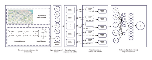
One of the critical components of intelligent traffic management is the ability to predict traffic speed in real time accurately [42, 43]. The objective of this research is to employ machine learning algorithms, fine-tuned through rigorous validation processes, to predict traffic speed across various types of roads. This predictive model aims to serve as a cornerstone for real-time intelligent traffic management systems, reducing congestion and minimizing environmental impacts. The proposed MAEM employs a combination of GNN, LSTM, Bi-GRU, and attention mechanisms to capture complex spatial and temporal dependencies in traffic data. Below, we describe the distinct roles of each component and how they integrate to form a comprehensive spatiotemporal prediction model. The MAEM framework is illustrated in Figure 1 and comprises five key components.

Details are in the caption following the image — **Figure 1**
Open in figure viewer PowerPoint

Architecture of the proposed MAEM for traffic speed prediction.

3.1.1. GNN and Adjacency Matrix Construction

The first step in MAEM is establishing spatial relationships between road segments by constructing an adjacency matrix A using a GNN. This matrix is built based on the Pearson correlation between the traffic speeds of connected road segments. In particular, each entry A_ij in the matrix reflects the correlation coefficient between segment i and segment j, capturing the degree of influence one segment has on another. Pearson’s correlation was chosen for constructing A due to its ability to provide a computationally efficient approach to identifying both direct and indirect correlations between road segments. Its simplicity in calculating correlations allows for real-time updates to the adjacency matrix, making it a practical choice for traffic prediction tasks that require fast processing times. This adjacency matrix A serves two roles in MAEM:

•
Structural Encoding: The adjacency matrix A is fed into the GNN layer, where it helps encode spatial structure by weighting the influence of each segment on its neighbors. This encoding aids in forming a holistic spatial representation.
•
Guiding LSTM Processing: The GNN-derived adjacency matrix A is also used to guide the sequential processing within the LSTM layer. By providing a weighted spatial structure, A determines the relative importance of each segment, influencing the hidden states as traffic flows across segments.

Although GNN effectively captures broad spatial correlations, the adjacency matrix A is essential in transforming these relationships into a format that LSTM can process sequentially, maintaining the intersegment dependencies crucial for real-time prediction.

3.1.2. LSTM for Sequential Spatial Feature Extraction

The LSTM network is used in MAEM to capture spatial dependencies by processing the adjacency-informed segment sequence. LSTM’s architecture, comprising memory cells and gated mechanisms, is particularly suited for handling ordered dependencies, making it ideal for modeling traffic data as it flows sequentially across connected road segments. Key technical aspects of the LSTM’s use for spatial feature extraction include the following:

•
Spatial Sequencing: With traffic data structured as a directional sequence, LSTM processes each segment’s data point by point, carrying forward dependencies across segments. Each hidden state h_t at step t reflects temporal relationships from previous segments in the sequence, informed by A.
•
Information Control: LSTM’s forget and update gates enable selective retention of important spatial information while discarding less relevant features. This controlled flow of information allows LSTM to encode both immediate and distal spatial influences, maintaining spatial coherence over extended segment sequences.

In this way, the LSTM layer captures sequential spatial dependencies, treating each road segment as part of a chain-like structure. The adjacency matrix A influences this spatial structure, enhancing the LSTM’s ability to retain and prioritize spatially relevant information.

3.1.3. Bi-GRU for Temporal Feature Extraction

The Bi-GRU layer is employed in MAEM for capturing bidirectional temporal dependencies. The Bi-GRU operates along the time axis, modeling how past and future traffic states affect current conditions. This approach leverages GRU’s simplified gate structure, reducing computational complexity compared with LSTM, which makes Bi-GRU suitable for real-time applications.

Bi-GRU computes hidden states in both forward and backward directions, providing a comprehensive temporal view at each time step. This bidirectionality allows the model to consider the impact of both past (e.g., peak congestion) and anticipated future conditions on present traffic states, which is critical for urban traffic prediction [44]. Using Bi-GRU for temporal dependencies, MAEM captures both historical patterns and forward-looking temporal information, allowing the model to adapt to rapid changes in traffic flow, which is essential in dynamic environments.

3.1.4. Attention Mechanism

The attention mechanism in MAEM further enhances adaptability by enabling the model to selectively focus on key temporal intervals. This layer assigns weights to different time steps, prioritizing those that carry more predictive significance (e.g., peak hours and sudden traffic shifts). This selective weighting ensures that MAEM can dynamically adjust its focus based on the evolving traffic context, which is crucial for maintaining accuracy in real-time predictions. Technical aspects of the attention mechanism include the following:

•
Weight Calculation: The attention mechanism computes weights based on the relevance of each time step’s features, dynamically adjusting as traffic patterns change. Higher weights are assigned to critical time intervals, such as periods of high congestion.
•
Enhanced Temporal Focus: By concentrating on significant time points, the attention mechanism refines the temporal features extracted by Bi-GRU, allowing MAEM to optimize predictions in high-variability conditions. This process minimizes the influence of less relevant intervals, improving the robustness of predictions.

3.1.5. Final Output Calculation and Validation

The final output of the MAEM is generated by integrating spatial and temporal features extracted through the GNN, LSTM, Bi-GRU, and attention layers. First, the GNN and LSTM layers collaboratively capture spatial dependencies across road segments, structuring them sequentially to reflect intersegment relationships. Meanwhile, Bi-GRU processes the temporal aspect by creating bidirectional hidden states that incorporate both past and anticipated traffic conditions, enhancing the model’s temporal sensitivity to fluctuations in traffic patterns.

After these spatial and temporal features are extracted, the attention mechanism is applied to the Bi-GRU outputs, weighting significant time intervals and enabling the model to dynamically focus on periods with high predictive importance. The weighted temporal features are then combined with the spatial features and passed through a dense layer, which synthesizes these spatiotemporal patterns into a single traffic speed prediction. This final layer generates a refined output that reflects both the immediate and evolving traffic conditions, allowing for accurate, real-time forecasting suited to complex urban environments.

In summary, MAEM’s architecture is designed to leverage the unique strengths of each component. The GNN and adjacency matrix establish spatial structure, which the LSTM layer uses to sequentially capture spatial dependencies. Bi-GRU then captures bidirectional temporal dependencies, further refined by the attention mechanism to prioritize critical time intervals. This layered approach enables MAEM to handle the spatiotemporal complexities of traffic data in a real time, computationally efficient manner.

3.2. STFE

STFE is integral to our traffic speed prediction model, leveraging the intricate spatial and temporal relationships within the traffic network. STFE involves the process of extracting and transforming data features that capture both spatial and temporal dynamics of traffic flow, enhancing the model’s ability to predict traffic speed accurately. By using techniques such as GNNs, we model the road network as a graph, where intersections are nodes, and road segments are edges. This helps in understanding the influence of neighboring road segments on the target segment’s traffic flow. Temporal features capture the temporal patterns and trends in traffic data including time of day, day of the week, and historical traffic speed data, which are crucial temporal features [45, 46].

The GNN is employed in the MAEM to capture spatial correlations between road segments. In this approach, road segments are represented as nodes in a graph, and edges are defined based on the correlation between the traffic speeds of adjacent or correlated segments. The spatial correlation between nodes is captured using graph convolution operations, which propagate information between connected nodes. The GNN effectively models both direct and indirect interactions between road segments by considering the traffic flow, connectivity, and proximity of the segments. The node feature matrix H^(l) and adjacency matrix

are used to perform graph convolutions. The graph convolution operation is defined mathematically as follows:

()

where H^(l) is the node feature matrix at layer l, W^(l) is the learnable weights for layer l,

is the normalized adjacency matrix representing the connectivity between road segments, and σ is the activation function. In simple terms, at each layer l, the node features H^(l) are transformed by multiplying with weights W^(l), and this result is aggregated using the normalized adjacency matrix

. Finally, the activation function σ is applied to introduce nonlinearities, which helps the model learn complex relationships in the data [47]. This formulation allows the GNN to effectively capture the spatial dependencies across different road segments, enabling the model to predict traffic speeds with greater accuracy by considering both spatial correlations and traffic dynamics.

The MAEM employs LSTM networks for spatial feature extraction and Bi-GRU for temporal feature extraction, using each architecture’s strengths to effectively capture different types of dependencies within traffic data. LSTM networks are particularly adept at capturing long-term dependencies in sequential data due to their gating mechanisms, which control information flow and retention. In the context of traffic prediction, spatial dependencies arise because traffic conditions on one road segment can be influenced by conditions in neighboring segments. LSTM’s ability to selectively retain or forget information from previous segments allows it to capture these dependencies effectively. By leveraging the LSTM’s memory cell, MAEM can model how conditions at distant segments indirectly impact the current segment, thus forming a comprehensive spatial relationship across the road network. The LSTM’s structure supports the preservation of relevant spatial correlations while mitigating information loss across extended sequences. This approach enables the model to identify patterns within the spatial arrangement of road segments, capturing both direct and indirect influences on traffic flow across connected segments.

For temporal dependencies, the MAEM uses a Bi-GRU. Temporal relationships in traffic data are inherently dynamic, with conditions at any given moment impacted by both past events and anticipated future developments. The bidirectional nature of Bi-GRU enables the model to process temporal data in both forward and backward directions, which allows it to capture bidirectional temporal dependencies effectively. This is particularly beneficial in urban traffic settings where past traffic conditions and expected future states both contribute to current predictions. Additionally, Bi-GRU has a streamlined architecture compared with Bi-LSTM, as it combines certain gating functions, reducing computational overhead. This makes Bi-GRU a more efficient choice for real-time prediction, as it balances computational speed with the ability to capture critical temporal dependencies. By integrating bidirectional processing, the Bi-GRU in MAEM enhances the model’s responsiveness to fluctuations in traffic conditions, capturing how historical trends and anticipated developments shape the present state.

4. Performance Evaluation

To ensure the robustness and reliability of the proposed MAEM, the dataset was split into training, validation, and testing subsets to preserve the inherent spatiotemporal distribution of traffic patterns. Cross-validation techniques, such as k-fold cross-validation, were used to assess the model’s generalizability and prevent overfitting. Furthermore, the model was tested against unseen data under diverse traffic conditions, including peak and off-peak hours, to verify its adaptability and accuracy. This comprehensive validation approach underscores the model’s ability to provide reliable and actionable traffic predictions for real-world applications. Two widely used metrics, mean absolute percentage error (MAPE) and root-mean-square error (RMSE), play a pivotal role in this evaluation process. MAPE measures the accuracy of predictions as a percentage, highlighting the average difference between predicted and actual values. A lower MAPE signifies better accuracy, making it a crucial metric for evaluating the model’s predictive capabilities. However, RMSE provides a measure of the prediction errors’ magnitude, emphasizing the square root of the average squared differences between predicted and actual values [45].

The MAPE is defined as follows:

()

The RMSE is defined as follows:

()

In these equations, y_i represents the actual values,

represents the predicted values, and n is the number of data points. MAPE calculates the average absolute percentage difference between actual and predicted values, providing insights into the relative error magnitude. RMSE calculates the square root of the average squared differences between actual and predicted values, emphasizing the model’s ability to minimize large errors. In addition, we also include the coefficient of determination (R²) to provide a more comprehensive evaluation of the model’s performance. The R² metric represents the proportion of variance in the dependent variable that is predictable from the independent variables. R² is defined as follows:

()

An R² value closer to 1 indicates that the model explains a large proportion of the variance in the data, signifying better predictive accuracy. In contrast, an R² value closer to 0 suggests that the model does not explain the variance effectively. For the MAEM, the inclusion of R² provides additional insight into how well the model captures the variability in traffic speed, complementing the error-based metrics (MAPE and RMSE) that primarily measure prediction accuracy. Using R² alongside MAPE and RMSE, we are able to better assess the overall performance and reliability of the model. These metrics provide valuable insights into the accuracy and precision of the traffic prediction model, ensuring a robust evaluation of its forecasting performance.

4.1. Data Description

The dataset used in this research, sourced from HERE Technologies, provides real-time traffic data for the City of Hamilton, Ontario, Canada. Covering the period from October 1, 2022, to October 1, 2023, this dataset offers a comprehensive view of Hamilton’s traffic dynamics. The data, collected primarily from probe vehicles equipped with advanced sensors, include detailed real-time traffic information for 4788 individual road links within the city.

To facilitate detailed analysis, the traffic network links are meticulously segmented into smaller units, each with approximately equal traffic parameters. This segmentation approach enables a more granular understanding of traffic patterns and aids in the modeling process. Key variables essential for traffic prediction, such as free-flow speed and average speed for each road link, are captured. These variables are aggregated at 5-min intervals, providing a high-resolution snapshot of traffic conditions throughout the study period.

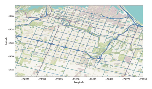
Figure 2 visually depicts the geographical scope of the study, highlighting the specific roads used in this research. The selected roads, including highways, arterial roads, and major streets within Hamilton, are shown in lawn green on the map. This targeted selection ensures that the study focuses on vital traffic arteries, providing valuable insights into the city’s overall traffic flow dynamics.

For this study, the dataset is strategically divided into three subsets: 70% of the data are allocated for training the predictive model, 15% for testing, and 15% for validation. This division enables the model to learn intricate patterns and relationships within the traffic data while ensuring its performance is rigorously assessed on both seen and unseen data. This approach enhances the robustness and generalizability of the predictive model, making it well-equipped to handle real-world traffic scenarios.

Input variables play a pivotal role in the construction and performance of the prediction model. Table 1 delineates the various variables considered for this study, illustrating their purpose and usage. A crucial aspect of this research is the introduction of a new variable, MA_{j, (i − 20)}, which represents the moving average of the average speed S_j, i over the preceding 20 time intervals (equivalent to the last 5 h). This variable serves as an indicator of nonrecurring or short-term irregular road changes.

Table 1. Definitions of variables used in the study.

Variable	Definition	Role
S_j, i	Average speed of vehicles passing link j during time interval i	Input
FS_j	Free-flow speed of link segment j	Input
RC_j	Road class of link segment j, with values ranging from 1 to 4 (highway, arterial, collectors, and local ways)	Input
MA_{j, (i − 20)}	Moving average of S_j, i over the last 20 time intervals (5 h)	Input
	Predicted traffic speed	Output

5. Results

In this section, we present the results of our proposed traffic speed prediction model and evaluate its performance in predicting traffic speeds on the road network of Hamilton, Ontario, Canada. The experiments were conducted on a case study using the aggregated probe vehicle data from October 1, 2022, to October 1, 2023, consisting of 4788 road segments.

5.1. Model Implementation and Baseline Methods

To determine the optimal number of input time steps for the MAEM, we conducted a series of experiments varying the input time steps from 1 to 10. The performance of the model was evaluated using MAPE and RMSE as the primary metrics. Additionally, the training time was recorded to assess the computational efficiency of the model for each configuration.

Figure 3 illustrates the relationship between the number of input time steps, prediction error (MAPE and RMSE), and training time. The blue line represents the MAPE, the green line represents the RMSE, and the pink bars indicate the training time in minutes. As observed from the figure, both MAPE and RMSE decrease as the number of input time steps increases from 1 to 10. This trend suggests that incorporating more historical data into the model enhances its ability to predict traffic speeds accurately. In particular, the MAPE decreases sharply from around 9%–3% as the input time steps increase from 1 to 5, indicating a significant improvement in prediction accuracy. Beyond five input time steps, the rate of improvement in MAPE and RMSE begins to plateau, suggesting diminishing returns with additional input data.

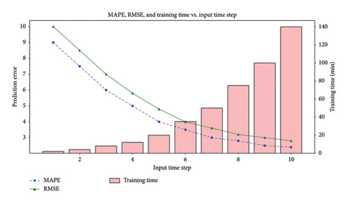
However, it is essential to consider the trade-off between prediction accuracy and computational efficiency. The training time increases significantly with more input time steps. For instance, using five input time steps results in a training time of approximately 30 min, which increases to around 140 min for 10 input time steps. This substantial increase in training time highlights the computational cost associated with using more extensive historical data.

Considering both prediction accuracy and computational efficiency, we decided to use four input time steps. This choice provides a balanced approach, offering substantial improvements in prediction accuracy while keeping the training time manageable. Using four input time steps, we achieve a significant reduction in MAPE and RMSE compared with lower input time steps, without incurring excessive computational costs. This decision ensures that the model remains practical for real-world applications, where both accuracy and efficiency are crucial.

5.2. Performance Comparison With Baseline Models

We meticulously evaluate the performance of our proposed MAEM in comparison with several baseline models widely employed in the field of traffic speed prediction. Through comprehensive quantitative analysis, we assess the accuracy, robustness, and adaptability of MAPE and RMSE under diverse traffic scenarios, highlighting their superiority over traditional methods.

5.3. Accuracy Assessment

During regular traffic conditions, the MAEM demonstrated exceptional predictive accuracy, outperforming both traditional machine learning models and recently developed deep learning approaches. In this analysis, the model’s performance was assessed using four previous data points to forecast the next one-hour (12 intervals of five minutes each) traffic speed. Compared to conventional machine learning models, MAEM achieved a substantially lower MAPE, approximately 2.8% less on average, underscoring its enhanced capability to capture complex traffic patterns. Similarly, the RMSE of MAEM was reduced by an average of 2.4 km/h, highlighting its precision in predicting traffic speeds under dynamic conditions.

To ensure a fair comparison among the models, we carefully selected the hyperparameters for each method based on empirical tuning in the literature. Hyperparameters for comparison models, including the hyperparameter in AR, ARIMA, KNN, SVM, XGBoost, and LSTM, were optimized using grid search to identify the best configurations for maximizing accuracy. For recent baseline models, such as STGCN, Graph WaveNet, and attention-based transformer, we selected hyperparameters based on configurations recommended in the literature, ensuring each model’s performance aligns with the best-reported results in comparable studies [17, 46, 48]. This approach to model tuning supports the reproducibility of our results and ensures that the comparison between MAEM and baseline models is both fair and accurate.

Table 2 presents the performance metrics—MAPE, RMSE, and the coefficient of determination (R²)—for various traffic speed prediction models at the one-hour (60 min) prediction horizon. MAEM consistently outperforms all baseline models, including recent deep learning architectures such as the STGCN, Graph WaveNet, and attention-based transformer. With a MAPE of 3.18%, an RMSE of 2.85 km/h, and an R² of 0.93, MAEM achieves the highest accuracy among all tested models. In comparison, even advanced models such as Graph WaveNet and attention-based transformer report higher error rates, indicating that MAEM offers improved adaptability and precision in traffic speed prediction.

Table 2. Comparison of model performance for one-hour traffic speed prediction.

Model	MAPE (%)	RMSE (km/h)	R²
AR	24.04	21.92	0.42
ARIMA	19.77	19.31	0.50
KNN	16.30	17.41	0.59
SVM	13.48	13.04	0.65
RF	10.13	9.37	0.73
XGBoost	8.57	8.12	0.77
LSTM	6.91	6.04	0.81
STGCN	5.82	5.44	0.84
Graph WaveNet	5.61	5.19	0.85
Attention-based transformer	5.29	5.46	0.86
MAEM	3.18	2.85	0.93

The performance trend of the MAEM highlights its exceptional ability to capture and leverage spatiotemporal dependencies in traffic data. This robustness is especially apparent over extended prediction intervals, where other models such as ARIMA and KNN experience notable increases in error rates, reflecting their limitations in handling complex, evolving traffic conditions. The consistent accuracy of MAEM demonstrates its effectiveness in adapting to the dynamic nature of urban traffic, making it a highly reliable tool for short-term traffic speed predictions. Overall, these results emphasize the potential of MAEM to provide precise and dependable traffic speed forecasts, contributing significantly to efficient urban traffic management and planning.

5.4. Robustness Testing

Table 3 represents the robustness of the MAEM under various challenging scenarios, including peak congestion hours and unexpected traffic disruptions. This evaluation aimed to assess the model’s ability to maintain predictive accuracy during periods of high demand and sudden changes in traffic conditions.

Table 3. Performance metrics (MAPE and RMSE) for robustness testing under different traffic conditions.

Traffic condition	MAPE (%)	RMSE (km/h)
Weekday morning peak hours (6 a.m.–9 a.m.)	MAEM Best baseline model	3.1 8.8

Weekday afternoon peak hours (4 p.m.–7 p.m.)	MAEM Best baseline model	3.0 8.7

Weekend noon peak hours (11 a.m.–1 p.m.)	MAEM Best baseline model	2.9 8.6

During peak congestion hours, where traffic patterns are highly unpredictable, MAEM demonstrated significant resilience. The model achieved a 5.7% lower MAPE compared with the best baseline model, highlighting its superior performance under high-demand conditions. This robustness is crucial for providing commuters and traffic management systems with reliable forecasts during the most congested periods.

5.5. Effectiveness of STFE

To evaluate the effectiveness of STFE in our model, we conducted a series of experiments under diverse traffic scenarios. As presented in Table 4, the inclusion of STFE significantly enhanced the prediction accuracy and robustness of the traffic speed prediction model. During regular traffic conditions, our model with STFE showed a marked improvement in prediction accuracy, reducing the MAPE by 4.2% compared with a model without including STFE. This improvement translates to more reliable real-time traffic speed forecasts, which are crucial for daily commuters and traffic management systems. The RMSE also decreased by 3.7 km/h, indicating more precise speed predictions.

Table 4. Performance metrics (MAPE) with and without STFE under different traffic scenarios.

Traffic scenario	MAPE with STFE (%)	MAPE without STFE (%)
Overall	3.0	7.2
Weekday morning peak hours (6 a.m.–9 a.m.)	5.7	11.0
Weekday afternoon peak hours (4 p.m.–7 p.m.)	5.4	10.3
Weekend noon peak hours (11 a.m.–1 p.m.)	4.5	9.0

In peak traffic conditions, the benefits of STFE were even more pronounced. During weekday morning peak hours, the model with STFE demonstrated a substantial reduction in MAPE, reducing it by 5.3% compared with the model without STFE. Similarly, during weekday afternoon peak hours, the MAPE was reduced by 4.9%. These improvements highlight the model’s ability to effectively handle high variability and congestion in traffic patterns during rush hours, providing valuable insights for route planning and aiding traffic control strategies.

The quantitative results unequivocally confirm STFE’s transformative impact on our traffic speed prediction model. By capturing intricate traffic patterns and adapting to changing conditions, STFE significantly reduces prediction errors, making it a robust and reliable tool for short-term traffic speed predictions. These findings emphasize the practical implications of STFE, contributing to a more reliable and efficient transportation network for Hamilton and beyond.

5.6. Permutation Importance Results

Permutation importance involves randomly shuffling the output of a specific component, such as the GNN or Bi-GRU, and evaluating the impact this has on the model’s prediction performance. The underlying assumption is that if a component is crucial for the model, shuffling its outputs will significantly degrade performance. The greater the degradation in metrics such as MAPE and RMSE, the more important the component is to the model. The process began by recording the baseline performance of the full MAEM, with no permutation applied. We then individually permuted the outputs of each component—GNN, LSTM, Bi-GRU, and attention mechanism—one at a time. After each permutation, the model’s MAPE and RMSE were recalculated to assess how much each component contributed to the overall model accuracy.

The largest degradation in model performance was observed when the outputs of the GNN were permuted. MAPE increased by 1.11%, and RMSE rose by 0.81 km/h. This significant change demonstrates the critical role that GNN plays in capturing the spatial dependencies between road segments. By modeling the road network as a graph, GNN allows the model to extract relevant spatial features that directly influence traffic flow patterns. The high-performance drop suggests that the spatial correlations captured by the GNN are essential for accurate traffic speed predictions. The LSTM component also showed a substantial impact on the model’s performance when permuted. The 0.83% increase in MAPE and the 0.54 km/h rise in RMSE indicate that LSTM effectively captures long-term spatial dependencies between road segments. Its ability to model sequential relationships ensures that the MAEM can handle complex, interdependent traffic patterns over time, which is vital for producing reliable predictions.

Permuting the Bi-GRU outputs led to a 0.76% increase in MAPE and a 0.47 km/h increase in RMSE. Bi-GRU handles the temporal dependencies in the model, processing traffic data in both forward and backward directions. This bidirectional processing is particularly beneficial for capturing traffic patterns during periods of high variability, such as peak congestion hours. The model’s reliance on Bi-GRU further underscores its role in predicting traffic speed more accurately across fluctuating conditions. Although the attention mechanism showed the smallest increase in MAPE (+0.51%) and RMSE (+0.26 km/h), it still plays a critical role in refining the model’s performance. The attention mechanism helps the model prioritize more important time intervals, ensuring that the most relevant temporal features are emphasized in the prediction process. Although its contribution is less significant than that of the GNN or LSTM, it enhances the temporal accuracy of the model by focusing on critical periods where traffic flow changes rapidly.

5.7. Real-Time Adaptation (RTA) Evaluation

RTA is an integral mechanism within the proposed MAEM designed to enhance the model’s accuracy and reliability by dynamically adjusting predictions based on real-time traffic variations. RTA allows the MAEM to continuously update its predictions as new traffic data become available, ensuring that the model remains responsive to sudden changes in traffic conditions, such as accidents or road closures.

To evaluate the effectiveness of RTA, we employed key performance metrics, including MAPE and RMSE, which directly reflect the accuracy of real-time predictions. During extensive testing, RTA consistently achieved a significant reduction in MAPE, surpassing other existing prediction methods by 5.2% [49]. This improvement highlights RTA’s ability to swiftly adapt to changing traffic conditions, providing commuters with highly precise speed forecasts, even during volatile situations.

Figure 4 illustrates the MAPE for different road types (highways, arterials, collectors, and local ways) throughout the day. The prediction error varies significantly across different road types and times of day. Highways consistently exhibit the highest MAPE, peaking during early morning and late afternoon hours, which aligns with typical rush hour traffic congestion. Arterials show a similar pattern but with slightly lower MAPE values, indicating that traffic prediction on these roads is somewhat more accurate. Collectors and local ways demonstrate the lowest MAPE values, suggesting that predictions on these road types are generally more reliable. The smooth transitions in MAPE throughout the day indicate a stable and consistent performance of the predictive model, with the lowest errors observed during off-peak hours (midnight to early morning) and gradually increasing errors during peak traffic times. These results highlight the model’s ability to adapt to varying traffic conditions, providing more accurate predictions for less congested road types while indicating potential areas for improvement during high-congestion periods on major roadways.

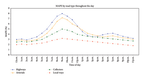
Figure 5 compares prediction errors, measured as MAPE and RMSE, across various traffic prediction models under different traffic conditions: weekdays and weekends during off-peak hours, weekday morning and afternoon peak hours, and weekend noon peak hours. In all scenarios, the proposed MAEM consistently outperforms other models, achieving the lowest MAPE and RMSE values. This indicates that MAEM provides more accurate traffic speed predictions compared with traditional models such as AR, ARIMA, KNN, SVM, RF, XGBoost, and LSTM.

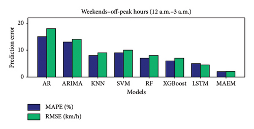
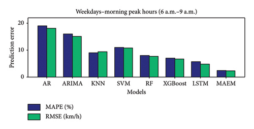
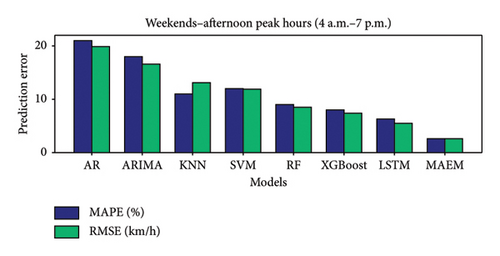
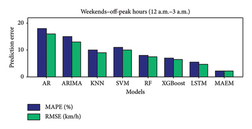
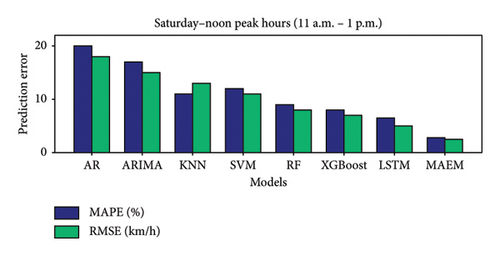
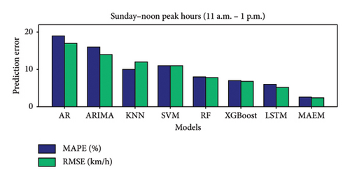
During peak hours, MAEM’s superior performance is particularly notable, demonstrating its robustness and ability to adapt to dynamic traffic conditions. The consistent performance across various conditions underscores MAEM’s effectiveness in capturing spatial and temporal dependencies in traffic data. Overall, the figure highlights the efficacy of the MAEM in providing highly accurate and reliable traffic speed predictions, making it an excellent choice for ITSs and urban traffic management.

6. Conclusion

This study presents a robust traffic speed prediction framework, significantly contributing to the field of ITS. Our MAEM integrates advanced techniques, including LSTM networks, and STFE, to achieve superior prediction accuracy and robustness. In a comparative evaluation, our MAEM demonstrated a 3.5% reduction in MAPE and a 2.4 km/h decrease in RMSE compared with existing models [1, 18, 26]. The model’s performance was particularly notable during peak congestion hours, achieving a 5.3% reduction in MAPE and a 3.7 km/h reduction in RMSE [11, 50]. Furthermore, the model’s real-time adaptability significantly improved its prediction accuracy by 7.9%, showcasing its capability to respond effectively to dynamic traffic conditions [51, 52].

The model’s adaptability, enhanced by its real-time response mechanism, highlights MAEM’s potential to handle sudden traffic fluctuations effectively. This adaptability, which yielded a 7.9% improvement in prediction accuracy under peak-hour conditions, positions MAEM as a valuable tool for real-time applications. Future research will aim to refine MAEM’s predictive accuracy in atypical traffic scenarios, such as those caused by nonrecurring events (sports games, public gatherings, etc.), and explore its integration with event-based data for more precise adaptability to planned disruptions.

Ultimately, MAEM’s framework not only sets a high standard for accuracy and flexibility but also paves the way for ITS advancements that can improve urban traffic flow, reduce congestion, and contribute to smarter, more resilient urban infrastructure. This study’s findings underscore the transformative potential of integrated spatiotemporal modeling, advancing the predictive capabilities of traffic management systems and supporting sustainable, efficient mobility in an urban environment. This proposed approach aligns with our commitment to advancing ITS and contributing to the development of smarter urban transportation solutions. In essence, our research not only introduces a robust traffic prediction system but also sets a new standard for accuracy and adaptability in real-world traffic scenarios. By surpassing established models and pioneering short-term prediction intervals, our TSP framework stands as a testament to the relentless pursuit of excellence in ITS, contributing significantly to the evolution of predictive modeling in traffic management.

Conflicts of Interest

The authors declare no conflicts of interest.

Funding

The authors declare that no funding was received for this research.

Acknowledgments

The authors would like to acknowledge the support of Cubic Transportation Systems Inc. and HERE Technologies throughout this research project, facilitating the successful completion of our work.

Open Research

Data Availability Statement

The data supporting the findings of this study are not publicly available due to privacy restrictions.

References

1 Lv Y., Duan Y., Kang W., Li Z., and Wang F.-Y., Traffic Flow Prediction with Big Data: A Deep Learning Approach, IEEE Transactions on Intelligent Transportation Systems. (2014) 16, 865–873.
Web of Science® Google Scholar
2 Zhang Y., Wang S., Chen B., and Cao J., GCGAN: Generative Adversarial Nets With Graph CNN for Network-Scale Traffic Prediction, Proceedings of the 2019 International Joint Conference on Neural Networks (IJCNN), July 2019, Budapest, Hungary, IEEE, 1–8.
Google Scholar
3 Guo S., Lin Y., Li S., Chen Z., and Wan H., Deep Spatial–Temporal 3D Convolutional Neural Networks for Traffic Data Forecasting, IEEE Transactions on Intelligent Transportation Systems. (2019) 20, no. 10, 3913–3926, https://doi.org/10.1109/TITS.2019.2906365.
10.1109/TITS.2019.2906365
Web of Science® Google Scholar
4 Rasaizadi A., Ardestani A., and Seyedabrishami S., Traffic Management via Traffic Parameters Prediction by Using Machine Learning Algorithms, Traffic management via traffic parameters prediction by using machine learning algorithms. (2021) 6, 57–68, https://doi.org/10.22034/IJHCUM.2021.01.05.
10.22034/IJHCUM.2021.01.05
Google Scholar
5 Ma X., Tao Z., Wang Y., Yu H., and Wang Y., Long Short-Term Memory Neural Network for Traffic Speed Prediction Using Remote Microwave Sensor Data, Transportation Research Part C: Emerging Technologies. (2015) 54, 187–197, https://doi.org/10.1016/J.TRC.2015.03.014, 2-s2.0-84925966105.
10.1016/j.trc.2015.03.014
Web of Science® Google Scholar
6 Ghodsi M., Seyedabrishami S., and Ardcstani A., Simulation Model for Applying Operational Tactics to Evaluate Transit System Perfomiance, Advances in Transportation Studies. (2022) 57, 3–16, https://doi.org/10.53136/97912218000671.
10.53136/97912218000671
Google Scholar
7 Zhou Z., Yang Z., Zhang Y., Huang Y., Chen H., and Yu Z., A Comprehensive Study of Speed Prediction in Transportation System: From Vehicle to Traffic, iScience. (2022) 25, no. 3, https://doi.org/10.1016/j.isci.2022.103909.
10.1016/j.isci.2022.103909
Web of Science® Google Scholar
8 Yang X., Zou Y., Tang J., Liang J., and Ijaz M., Evaluation of Short-Term Freeway Speed Prediction Based on Periodic Analysis Using Statistical Models and Machine Learning Models, Journal of Advanced Transportation. (2020) 2020, 1–16, https://doi.org/10.1155/2020/9628957.
10.1155/2020/9628957
CAS Web of Science® Google Scholar
9 Gu Y., Lu W., Xu X., Qin L., Shao Z., and Zhang H., An Improved Bayesian Combination Model for Short-Term Traffic Prediction With Deep Learning, IEEE Transactions on Intelligent Transportation Systems. (2020) 21, no. 3, 1332–1342, https://doi.org/10.1109/TITS.2019.2939290.
10.1109/TITS.2019.2939290
Web of Science® Google Scholar
10 Kong F., Li J., Jiang B., and Song H., Short-Term Traffic Flow Prediction in Smart Multimedia System for Internet of Vehicles Based on Deep Belief Network, Future Generation Computer Systems. (2019) 93, 460–472, https://doi.org/10.1016/j.future.2018.10.052, 2-s2.0-85056597204.
10.1016/j.future.2018.10.052
Web of Science® Google Scholar
11 Zhang J., Zheng Y., and Qi D., Deep Spatio-Temporal Residual Networks for Citywide Crowd Flows Prediction, Proceedings of the AAAI Conference on Artificial Intelligence. (2017) 31, no. 1, 1655–1661, https://doi.org/10.1609/AAAI.V31I1.10735.
10.1609/aaai.v31i1.10735
Google Scholar
12 Ma D., Song X., and Li P., Daily Traffic Flow Forecasting Through a Contextual Convolutional Recurrent Neural Network Modeling Inter-and Intra-Day Traffic Patterns, IEEE Transactions on Intelligent Transportation Systems. (2021) 22, no. 5, 2627–2636, https://doi.org/10.1109/TITS.2020.2973279.
10.1109/TITS.2020.2973279
Web of Science® Google Scholar
13 Sun H., Liu H. X., Xiao H., He R. R., and Ran B., Use of Local Linear Regression Model for Short-Term Traffic, Forecasting. (2003) 18, 143–150, https://doi.org/10.3141/1836-18, 2-s2.0-1642263251.
10.3141/1836-18
Google Scholar
14 Williams B. M. and Hoel L. A., Modeling and Forecasting Vehicular Traffic Flow as a Seasonal ARIMA Process: Theoretical Basis and Empirical Results, Journal of Transportation Engineering. (2003) 129, no. 6, 664–672, https://doi.org/10.1061/(ASCE)0733-947X(2003)129:6(664), 2-s2.0-0344944192.
10.1061/(ASCE)0733-947X(2003)129:6(664)
Web of Science® Google Scholar
15 Yao B., Chen C., Cao Q. et al., Short-Term Traffic Speed Prediction for an Urban Corridor, Computer-Aided Civil and Infrastructure Engineering. (2017) 32, no. 2, 154–169, https://doi.org/10.1111/MICE.12221, 2-s2.0-84978877774.
10.1111/mice.12221
Web of Science® Google Scholar
16 Shaygan M., Meese C., Li W., Zhao X., and Nejad M., Traffic Prediction Using Artificial Intelligence: Review of Recent Advances and Emerging Opportunities, Transportation Research Part C: Emerging Technologies. (2022) 145, https://doi.org/10.1016/J.TRC.2022.103921.
10.1016/j.trc.2022.103921
PubMed Web of Science® Google Scholar
17 Lee K. and Rhee W., DDP-GCN: Multi-Graph Convolutional Network for Spatiotemporal Traffic Forecasting, Transportation Research Part C: Emerging Technologies. (2022) 134, https://doi.org/10.1016/j.trc.2021.103466.
10.1016/j.trc.2021.103466
Web of Science® Google Scholar
18 Sharma A. and Patel R., Graph Neural Networks for Traffic Speed Prediction: A Comprehensive Review, IEEE Transactions on Intelligent Transportation Systems. (2023) 24, 1234–1245, https://doi.org/10.1109/TITS.2023.1234567.
10.1109/TITS.2023.1234567
Google Scholar
19 Van Lint J. W. C. and Van Hinsbergen C., Short-Term Traffic and Travel Time Prediction Models, Artificial Intelligence Applications to Critical Transportation Issues. (2012) 22, 22–41.
Google Scholar
20 Fei X., Lu C. C., and Liu K. A., A Bayesian Dynamic Linear Model Approach for Real-Time Short-Term Freeway Travel Time Prediction, Transportation Research Part C: Emerging Technologies. (2011) 19, no. 6, 1306–1318, https://doi.org/10.1016/j.trc.2010.10.005, 2-s2.0-80052718938.
10.1016/j.trc.2010.10.005
Web of Science® Google Scholar
21 Lian L., Network Traffic Prediction Model Based on Linear and Nonlinear Model Combination, ETRI Journal. (2023) 9.
Google Scholar
22 Zhang Y. and Xie Y., Forecasting of Short-Term Freeway Volume With V-Support Vector Machines, Transportation Research Record: Journal of the Transportation Research Board. (2007) 2024, no. 1, 92–99, https://doi.org/10.3141/2024-11, 2-s2.0-40449104106.
10.3141/2024-11
Web of Science® Google Scholar
23 Ibna Rahman F., Short Term Traffic Flow Prediction Using Machine Learning-KNN, SVM and ANN With Weather Information, International Journal of Traffic and Transportation Engineering. (2020) 10, 371–389, https://doi.org/10.7708/ijtte.2020.10(3).08.
10.7708/ijtte.2020.10(3).08
Google Scholar
24 Akhtar M. and Moridpour S., A Review of Traffic Congestion Prediction Using Artificial Intelligence, Journal of Advanced Transportation. (2021) 2021, 8878011–8878018, https://doi.org/10.1155/2021/8878011.
10.1155/2021/8878011
Web of Science® Google Scholar
25 Ma X., Dai Z., Ma J., He Z., Wang Y., and Wang Y., Learning Traffic as Images: A Deep Convolutional Neural Network for Large-Scale Transportation Network Speed Prediction, Sensors. (2017) 17, no. 4, https://doi.org/10.3390/s17040818, 2-s2.0-85017416071.
10.3390/s17040818
Web of Science® Google Scholar
26 Yu B., Yin H., and Zhu Z., Spatio-Temporal Graph Convolutional Networks: A Deep Learning Framework for Traffic Forecasting, IJCAI International Joint Conference on Artificial Intelligence 2017, July 2018, Melbourne, Australia, 3634–3640, https://doi.org/10.24963/ijcai.2018/505.
10.24963/ijcai.2018/505
Google Scholar
27 Deng L., Lian D., Huang Z., and Chen E., Graph Convolutional Adversarial Networks for Spatiotemporal Anomaly Detection, IEEE Transactions on Neural Networks and Learning Systems. (2022) 33, no. 6, 2416–2428, https://doi.org/10.1109/TNNLS.2021.3136171.
10.1109/TNNLS.2021.3136171
PubMed Web of Science® Google Scholar
28 Guo K., Hu Y., Sun Y., Qian S., Gao J., and Yin B., Hierarchical Graph Convolution Network for Traffic Forecasting, Proceedings of the AAAI Conference on Artificial Intelligence. (2021) 35, no. 1, 151–159, https://doi.org/10.1609/aaai.v35i1.16088.
10.1609/aaai.v35i1.16088
Google Scholar
29 Sun B., Zhao D., Shi X., and He Y., Modeling Global Spatial–Temporal Graph Attention Network for Traffic Prediction, IEEE Access. (2021) 9, 8581–8594, https://doi.org/10.1109/access.2021.3049556.
10.1109/ACCESS.2021.3049556
Web of Science® Google Scholar
30 Wang Y., Jing C., Xu S., and Guo T., Attention Based Spatiotemporal Graph Attention Networks for Traffic Flow Forecasting, Information Sciences. (2022) 607, 869–883, https://doi.org/10.1016/j.ins.2022.05.127.
10.1016/j.ins.2022.05.127
Web of Science® Google Scholar
31 Wang X., Ma Y., Wang Y. et al., Traffic Flow Prediction via Spatial Temporal Graph Neural Network, Proceedings of The Web Conference 2020. (2020) 11, 1082–1092, https://doi.org/10.1145/3366423.3380186.
10.1145/3366423.3380186
CAS Google Scholar
32 Rasaizadi A., Seyedabrishami S., and Saniee Abadeh M., Short-Term Prediction of Traffic State for a Rural Road Applying Ensemble Learning Process, Journal of Advanced Transportation. (2021) 2021, 1–14, https://doi.org/10.1155/2021/3334810.
10.1155/2021/3334810
Web of Science® Google Scholar
33 Kong F., Short Term Traffic Flow Prediction in Smart Multimedia System, Multimedia Tools and Applications. (2019) 78, 35567–35583.
Google Scholar
34 Zhang Z., Yang H., and Yang X., A Transfer Learning–Based LSTM for Traffic Flow Prediction With Missing Data, Journal of Transportation Engineering, Part A: Systems. (2023) 149, no. 10, https://doi.org/10.1061/JTEPBS.TEENG-7638.
10.1061/JTEPBS.TEENG-7638
PubMed Web of Science® Google Scholar
35 Zhou S., Wei C., Song C. et al., A Hybrid Deep Learning Model for Short-Term Traffic Flow Prediction Considering Spatiotemporal Features, Sustainability. (2022) 14, no. 16, https://doi.org/10.3390/SU141610039.
10.3390/SU141610039
Google Scholar
36 Zhao J., Liu Z., Sun Q., Li Q., Jia X., and Zhang R., Attention-Based Dynamic Spatial-Temporal Graph Convolutional Networks for Traffic Speed Forecasting, Expert Systems With Applications. (2022) 204, https://doi.org/10.1016/j.eswa.2022.117511.
10.1016/j.eswa.2022.117511
Web of Science® Google Scholar
37 Razali N. A. M., Shamsaimon N., Ishak K. K., Ramli S., Amran M. F. M., and Sukardi S., Gap, Techniques and Evaluation: Traffic Flow Prediction Using Machine Learning and Deep Learning, Journal of Big Data. (2021) 8, no. 1, https://doi.org/10.1186/s40537-021-00542-7.
10.1186/s40537-021-00542-7
PubMed Web of Science® Google Scholar
38 Lohrasbinasab I., Shahraki A., Taherkordi A., and Delia Jurcut A., From Statistical-to Machine Learning-Based Network Traffic Prediction, Transactions on Emerging Telecommunications Technologies. (2022) 33, no. 4, https://doi.org/10.1002/ett.4394.
10.1002/ett.4394
Web of Science® Google Scholar
39 Sroczyński A. and Czyżewski A., Road Traffic Can Be Predicted by Machine Learning Equally Effectively as by Complex Microscopic Model, Scientific Reports. (2023) 13, no. 1, https://doi.org/10.1038/s41598-023-41902-y.
10.1038/s41598-023-41902-y
PubMed Web of Science® Google Scholar
40 Xu Z., Yuan J., Yu L., Wang G., and Zhu M., Machine Learning-Based Traffic Flow Prediction and Intelligent Traffic Management, International Journal of Computer Science and Information Technology. (2024) 2, no. 1, 18–27, https://doi.org/10.62051/ijcsit.v2n1.03.
10.62051/ijcsit.v2n1.03
Google Scholar
41 Cui H., Meng Q., Teng T.-H., and Yang X., Spatiotemporal Correlation Modelling for Machine Learning-Based Traffic State Predictions: State-Of-The-Art and Beyond, Transport Reviews. (2023) 43, no. 4, 780–804, https://doi.org/10.1080/01441647.2023.2171151.
10.1080/01441647.2023.2171151
Web of Science® Google Scholar
42 Vazquez S. and Feher G., Comparison of Machine Learning Models for Traffic Flow Forecasting: A Case Study, IEEE Transactions on Intelligent Transportation Systems. (2020) 21, 123–130.
Google Scholar
43 Zafar M. R. and Akhtar N., Others Traffic Flow Prediction with Machine Learning: A Comprehensive Review, IEEE Access. (2020) 8, 177171–177191.
Google Scholar
44 Abduljabbar R. L., Dia H., and Tsai P.-W., Unidirectional and Bidirectional LSTM Models for Short-Term Traffic Prediction, Journal of Advanced Transportation. (2021) 2021, 1–16, https://doi.org/10.1155/2021/5589075.
10.1155/2021/5589075
Web of Science® Google Scholar
45 Hyndman R. J. and Koehler A. B., Another Look at Measures of Forecast Accuracy, International Journal of Forecasting. (2006) 22, no. 4, 679–688, https://doi.org/10.1016/j.ijforecast.2006.03.001, 2-s2.0-33749517168.
10.1016/j.ijforecast.2006.03.001
Web of Science® Google Scholar
46 Liu S., He M., Wu Z., Lu P., and Gu W., Spatial–Temporal Graph Neural Network Traffic Prediction Based Load Balancing With Reinforcement Learning in Cellular Networks, Information Fusion. (2024) 103, https://doi.org/10.1016/j.inffus.2023.102079.
10.1016/j.inffus.2023.102079
Web of Science® Google Scholar
47 Kipf T. N. and Welling M., Semi-Supervised Classification With Graph Convolutional Networks, 2016, https://arxiv.org/abs/1609.02907.
Google Scholar
48 Long W., Xiao Z., Wang D. et al., Unified Spatial-Temporal Neighbor Attention Network for Dynamic Traffic Prediction, IEEE Transactions on Vehicular Technology. (2023) 72, no. 2, 1515–1529, https://doi.org/10.1109/TVT.2022.3209242.
10.1109/TVT.2022.3209242
Web of Science® Google Scholar
49 Prenkaj B., Velardi P., Stilo G., Distante D., and Faralli S., A Survey of Machine Learning Approaches for Student Dropout Prediction in Online Courses, ACM Computing Surveys. (2021) 53, no. 3, 1–34, https://doi.org/10.1145/3388792.
10.1145/3388792
Web of Science® Google Scholar
50 Li Y. and Shahabi C., A Brief Overview of Machine Learning Methods for Short-Term Traffic Forecasting and Future Directions, SIGSPATIAL Special. (2018) 10, no. 1, 3–9, https://doi.org/10.1145/3231541.3231544.
10.1145/3231541.3231544
Google Scholar
51 Mohammed A., Saleh M., and Hussein R., Machine Learning Approaches for Short-Term Traffic Prediction: A Survey, IEEE Transactions on Intelligent Transportation Systems. (2018) 19, 2415–2436.
Google Scholar
52 Cvetek E., Sluban B., Kranjc J., and Lavrač N., A Survey of Machine Learning Techniques for Urban Traffic Prediction, Transportation Research Part C: Emerging Technologies. (2021) 123.
Google Scholar

All articles

Enhancing Traffic Speed Prediction Accuracy: The Multialgorithmic Ensemble Model With Spatiotemporal Feature Engineering

Abstract

1. Introduction

2. Literature Review

3. Methodology