Volume 2025, Issue 1 7897020

Research Article

Open Access

Optimization of Skip-Stop Train Schedule in Urban Rail Transit Under Virtual Coupling

Jiawei Bai,

Jiawei Bai

orcid.org/0009-0003-6596-5524

School of Traffic and Transportation , Beijing Jiaotong University , Beijing , 100044 , China , njtu.edu.cn

The Line Branch Company , Beijing Mass Transit Railway Operation Corporation , Beijing , 100082 , China

Search for more papers by this author

Qi Zhang,

Corresponding Author

Qi Zhang

[email protected]

orcid.org/0000-0003-2385-6787

School of Traffic and Transportation , Beijing Jiaotong University , Beijing , 100044 , China , njtu.edu.cn

Search for more papers by this author

Jiawei Bai,

Jiawei Bai

orcid.org/0009-0003-6596-5524

School of Traffic and Transportation , Beijing Jiaotong University , Beijing , 100044 , China , njtu.edu.cn

The Line Branch Company , Beijing Mass Transit Railway Operation Corporation , Beijing , 100082 , China

Search for more papers by this author

Qi Zhang,

Corresponding Author

Qi Zhang

[email protected]

orcid.org/0000-0003-2385-6787

School of Traffic and Transportation , Beijing Jiaotong University , Beijing , 100044 , China , njtu.edu.cn

Search for more papers by this author

First published: 16 April 2025

https://doi.org/10.1155/atr/7897020

Citations: 2

Academic Editor: Peter J. Jin

Share a link

Email
Wechat
Bluesky

Abstract

Virtual coupling technology enables decoupling and coupling operations of trains more flexible, and the tracking interval between trains is also shortened. This paper analyzes the advantages of virtual coupling technology in the application of skip-stop operation, and operation strategies based on real-time train coupling and decoupling are proposed. With the goal of minimizing the total travel time of passengers, an optimization model for skip-stop timetable under virtual coupling technology is established, which limits the virtual operation location, the number of virtual coupling and decoupling, and the relationship between virtual operation and arrival and departure status of trains. At the same time, an adaptive large-scale neighborhood search algorithm was designed for model solving. A case study of certain urban rail transit line R, which is a skip-stop-operated urban rail transit line, has been carried out. The model and algorithm were validated using real data from the morning peak hour, and the results show that the application of virtual coupling technology can effectively reduce the total travel time of passengers. Under the conditions of this case study, virtual coupling technology can improve service quality. In actual operation, under suitable passenger flow and line conditions, the reasonable use of virtual coupling technology to improve the skip-stop operation mode can improve the service quality and operational efficiency of urban rail transit.

1. Introduction

With the development of the economy and society, the rail transit network continues to extend, and long lines of rail transit continue to emerge. The distribution of passenger demand in time and space has obvious imbalance, and the traditional all-stop organization is no longer able to meet the passenger demand. To cope with this situation, many international metropolises have adopted a skip-stop operation and have achieved some successful experiences, such as the Tsukuba Line in Japan, the RER Line in Paris [1], and the Market-Frankfurt Line of the Philadelphia Metro (https://www.septa.org). According to skip-stop operation, some skip-stop trains are often operated while operating some all-stop trains. Due to skipping some stations with lower passenger demand, skip-stop trains can save several acceleration, deceleration, and dwell times caused by stops [2]. The skip-stop operation can effectively save travel time for long-distance passengers and reduce operating costs [3]. Some scholars have explored the application mode of the skip-stop operation to better adapt to passenger demand [4]. However, the waiting time of passengers at overtaking stations has also been extended to some extent [5], and the service level has been reduced. In order to improve the skip-stop operation, we can consider using virtual coupling technology, a new and flexible technology, to change the overtaking mode and timetable design method of the existing skip stop operation.

The concept of virtual coupling train originally originated from the “virtual coupled train formations” proposed by BOCK et al. [6], which used wireless communication instead of mechanical coupling. Through wireless communication between trains, the following trains of the virtual coupling train can obtain the running status of the leading train and maintain a certain distance for operation. On the basis of the “train–ground–train” communication structure, virtual coupling technology has been added with “train–train” communication, which means direct communication between trains. It can enable trains to exchange real-time information such as position and speed and independently calculate train movement authorization. The flexibility of the real-time online coupling and decoupling of virtual coupling trains can better adapt to different operating modes. Many researchers believe that virtual coupling technology will bring significant changes to existing operating modes [7–10]. In recent years, some researchers have begun to study the application of virtual coupling technology in train operation control, train communication, and transportation organization (see Section 2) and have achieved certain results. However, there is still a lack of research on the impact of applying virtual coupling technology on skip-stop operation.

Therefore, this paper analyzes the possible changes in skip-stop operation after applying virtual coupling technology. We construct a mathematical model to study the optimization problem of skip-stop operation schedule under the application of virtual coupling technology in order to explore the impact of virtual coupling technology on the transportation efficiency of skip stop operations and we explore the corresponding solving approach, so as to provide a reference for the practice in similar scenarios.

The remainder of this paper is organized as follows. In Section 2, we will conduct the literature review on virtual coupling technology. In Section 3, the skip-stop operation strategies, applying virtual coupling technology, based on real-time coupling and decoupling are analyzed, and the basic scenario of the problem is described. Section 4 constructs a timetable optimization model. In Section 5, a hybrid algorithm based on the adaptive large neighborhood search (ALNS) algorithm is proposed for solving the model. In Section 6, a numerical experiment is conducted through a practical case. Finally, Section 7 draws conclusions and discusses future research directions.

2. Literature Review

Virtual coupling technology has brought opportunities to the railway industry, not only enriching existing train control technologies [11] and transportation organization but also posing significant challenges to existing communication technologies [12]. It was found that academic research mainly focuses on control and communication systems [13]. In addition, the literature review will also focus specifically on the transportation organization of virtual coupling trains.

2.1. Train Operation Control and Communication Technology

Many researchers have analyzed existing train control technologies and found that virtual coupling trains can shorten train tracking intervals in a more intelligent and flexible manner [14–17]. Liu et al. [18, 19] proposed a coordinated control method using the idea of virtual coupling based on multiagent system (MAS) to achieve stable tracking of trains. The simulation results show that this method can ensure the safety of operation, shorten train operation intervals, and improve operation control efficiency. Prak et al. [20] proposed a tracking interval control model with robustness under the application of virtual coupling technology and developed a gap reference generation scheme to ensure the merge and separation of two trains. The simulation results show that the method proposed is effective. Quaglietta et al. [21] constructed a train-following model considered nonlinear train dynamics and relevant factors based on the application of virtual coupling technology. A case study has been conducted for a portion of the South West Main Line in the UK, and the results showed that virtual coupling technology may have certain advantages in train capacity utilization and other aspects. Xiaolin Luo et al. [22] proposed a distributed adaptive model predictive control (AMPC) system for coordinating the driving of each unit train in virtual coupling. The simulation results show that the proposed AMPC system has better performance and can make the trains track the desired objective well. Cao et al. [23] built a control model for leaders and followers based on the longitudinal dynamic model of a virtual coupling single train, and the generalized model predictive control and mixed artificial potential field are used to control the virtual coupling formation and the trains in the formation. Through simulation experiments based on the Beijing–Shanghai high-speed railway, it has been proven that the method can ensure the operation safety of virtual coupled train. Wang et al. [24] built a virtually coupled train set (VCTS) architecture-based industrial Internet of Things and applied reinforcement learning (RL) to avoid trapping into a local optimization. Simulation results confirmed that the proposed RL-based cooperative control approach would achieve small distance tracking between trains. Liu et al. [25] proposed a hierarchical control approach with a two-layer framework. In the upper and lower layers, a trajectory planning method and a model predictive control method were designed separately to ensure that each unit accurately tracks the specified trajectory in real time. Field tests have shown that this method leads to a breakthrough reduction of the following distance between two units in VCTS to less than 105 m at a speed of 80 km/h. There are also some studies combining model predictive control with long and short-term memory neural networks to improve the tracking accuracy and stability of train convoys [26] and reduce the speed differences and position differences of tracking trains [27].

In terms of communication technology, the EU has compared different solutions and pointed out that 5G technology is an important direction for future virtual coupling communication technology in Europe [28]. Ma et al. [29] develop an event trigger control (ETC) method to mitigate effects of jamming attacks on VCTS. Simulation results demonstrate that ETC can ensure the stable headway between adjacent trains and improve the transportation efficiency.

2.2. Transportation Organization

Virtual coupling technology is believed to better adapt to the spatiotemporal imbalance of passenger flow due to its unique flexibility. Schuman [30] proposed several modes of virtual coupling and decoupling using new types of turnouts. The simulation tool DFSimu was used to verify the advantages of virtual coupling technology applied on Shinkansen in Japan. The results showed that the application of virtual coupling technology can effectively improve the transport capacity of Shinkansen. Liu et al. [31] proposed a dynamic coupling method for coordinating and scheduling virtual coupling trains, which has been proven to reduce the product of vacant seats and mileage of trains traveling on routes with uneven distribution of passenger flow in time and space. Wang et al. [32] proposed a carrying capacity calculation method based on the parallel train diagram that adapts to flexible train formation technology. According to the verification, the variable formation based on virtual coupling has the least impact on the carrying capacity. Cao et al. [33] proposed a dynamic coupling and decoupling and scheduling scheme using virtual coupling technology based on the dynamic passenger flow of urban rail transit and proved that virtual coupling technology can significantly improve the transportation efficiency of urban rail transit trains.

In terms of transportation organization and scheduling, various studies have been conducted on different types of routes and scenarios. Lee et al. [34] proposed a train operation plan using virtual coupling technology and provided an algorithm for generating train operation plans. The analysis results indicate that the proposed operation plan can effectively improve the average speed of trains and the transport capacity of the line. Gallo et al. [35] proposed a mathematical model to optimize the number of virtual coupling trains on a circle railway line with a single track. The verification results indicate that the virtual coupling technology can contribute to designing more flexible services in railways and avoid wasting resources (i.e. trains and infrastructure) while meeting the transport demand. Muniandi [33] described seven different virtual coupling strategies and verified the effectiveness of the proposed system and method through theoretical analysis and case simulation. Gallo et al. [34] proposed a railway passenger service model in a scenario where virtual coupling technology is applied, with the goal of minimizing the number of transfer passengers, to determine the optimal path and departure time of trains in the urban railway network. You and Yang [35] proposed several operation modes suitable for virtual coupling trains, and the validation results on the Beijing Metro Batong Line showed that the operation scheme using virtual coupling technology can effectively shorten passenger travel time. Chen et al. [36] proposed an integrated train scheduling method and used a multiobjective optimization model to optimize the train schedule. The numerical results show that the proposed method can improve schedule punctuality and reduce the number of stranded passengers effectively. Zhang innovatively developed a VC-enabled train-centric simulation flow and algorithms and designed experiment on the NetLogo platform. Zhang [37] proposed a mathematical formula for the calculation of the train operation cost, passenger travel cost, and passenger comfort degree. And the conditions for train platooning under virtual coupling are synthesized [38]. The numerical simulation results have verified the effectiveness of the proposed method.

Overall, the study on the application of virtual coupling technology in traditional skip-stop operation is still blank. Moreover, the existing studies on virtual coupling technology in transportation organization mainly focus on simulation methods, and there is relatively little study on the application of heuristic algorithms in this area. The main contributions of this article are as follows:

1.
Analyze the application of virtual coupling technology in traditional skip-stop operation. The organizational strategies of using and not using overtaking lines have been proposed. The method of train coupling and decoupling under virtual coupling technology has been proposed, indicating that compared to traditional technology, virtual coupling technology has more flexibility in online coupling and decoupling.
2.
Constructed an optimization model for skip-stop operation schedule under virtual coupling. Set constraints on safety headway based on the state of the trains when they arrive at or depart from the station. For virtual operations, constraints have been added to limit the coupling and decoupling operations and the state of the trains.
3.
Design heuristic algorithms suitable for solving models. Apply ALNS to the optimization of skip-stop train schedule under virtual coupling. Designed destroy and repair operators based on the selection of virtual operation location and the inserting or removal of trains. Combining destroy and repair operators for neighborhood search based on the paired appearance of virtual coupling operations.

3. Analysis of Skip-Stop Operation Using Virtual Coupling Technology

The skip-stop service considered in this study consists of operating trains alternately as train a, which is a skip-stop train, and train b, which is an all-stop train. After the application of virtual coupling technology, the overtaking line can be used or not by skip-stop operation to make train a and train b run on the same line.

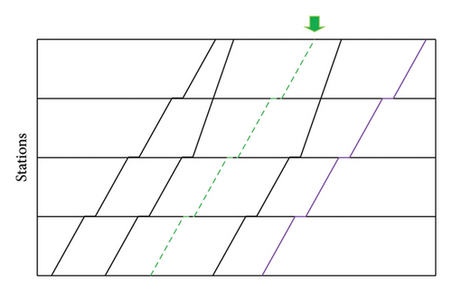
The skip-stop operation process without using overtaking lines under the application of virtual coupling technology is shown in Figure 1. Virtual coupling trains are virtually decoupled into two independent trains in a section or station. The leading train passes through some stations without stopping, catching up with the train ahead and operating a virtual coupling with it.

Details are in the caption following the image — **Figure 1**
Open in figure viewer PowerPoint

Skip-stop operation applying virtual coupling (no overtaking).

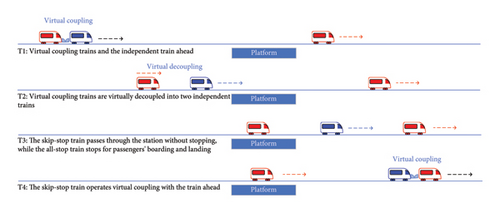
The skip-stop operation without using overtaking lines does not require specialized overtaking equipment on the line, allowing skip-stop trains and all-stop trains to operate together on the main line. However, due to the fact that the skip-stop train changes from a “leader” to a “follower” during its operation, it cannot overtake the all-stop train ahead after the first virtual decoupling operation. Therefore, it is necessary to comprehensively consider the train’s operating speed, stopping plan, and specific conditions of the route to determine whether this mode is suitable.

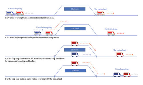
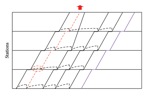
The skip-stop operation mode under the application of virtual coupling technology using overtaking lines operates virtual operations of trains at stations or sections on the basis of traditional mode. The specific process is shown in Figure 2. Virtual coupling trains are divided into two independent trains in the section or station. After arriving at the overtaking station, the all-stop train enters the siding and stops for passengers to board and alight. The skip-stop train quickly passes through the station without stopping and operates virtual coupling with the train ahead according to the situation. This skip-stop operation mode can be combined with the aforementioned mode that does not use overtaking lines.

4. Mathematical Modeling

4.1. Problem Statement

4.1.1. Passenger Choice Behavior

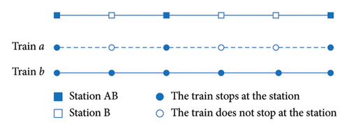
The stations of urban rail transit lines using skip-stop operation can be divided into station AB, where all trains stop, and station B, where only trains b stop, as shown in Figure 3.

According to the types of passengers’ origin and destination stations, passengers can be divided into four categories (P₁, P₂, P₃, P₄), as shown in Table 1. Passengers can choose to take direct trains or non-direct trains that need to be transferred at subsequent stations based on their train capacity and preferences. In order to shorten the total travel time of passengers, the study assumes that passengers who need to transfer will transfer from train b to train a at the first AB station after the origin and from train a to train b at the last AB station before the destination. Considering that frequent boarding and alighting during transfers bring additional transfer time and reduce passengers′ travel experience, the study assumes that passengers can only accept one transfer.

Table 1. Passenger path selection type.

Origin-destination	P₁ (AB-AB)	P₂ (AB-B)	P₃ (B-AB)	P₄ (B-B)
Path types that can be selected	1. a	1. a-b	1. b	1. b
	2. b	2. b	2. b-a
	3. b-a

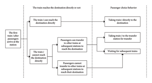
For passenger choice behavior, many scholars have adopted logit model for research [39–41]. Based on the above analysis, as illustrated in Figure 4, if the current train can directly reach the destination, passengers will prioritize taking the train. Otherwise, based on whether passengers can transfer to other trains at subsequent stations after taking the current train, passengers are assigned to transfer or wait for subsequent trains according to the logit model.

4.1.2. Definition of the Research Question

In this study, the optimization problem of skip-stop train schedule under virtual coupling technology can be defined as finding a solution where virtual operations are carried out in urban rail transit, as well as when trains arrive and depart, with the objective of minimizing passenger travel time.

Consider a unidirectional single-track urban rail transit line corridor with N stations. The train capacity, total number of available trains, number and location of stations with overtaking lines, and running data are already known. Passenger demand is defined as the origin–destination–time form and is given as input. The output optimized solution consists of the number of different types of trains, the plan for overtaking and virtual operations, and the departure and arrival times of trains. It should be noted that the timetable we output is adjusted before the train operation. The corresponding decision variables are defined as follows:

•
;
•
;
•
: arrival time of train i at station n;
•
: departure time of train i at station n.

Also, we will need the notations and parameters shown in Table 2.

Table 2. Constants, parameters, and auxiliary variables.

Constants and parameters
i, j	Index of trains, i, j ∈ I;
n, m	Index of stations, n, m ∈ N;
h	The minimum safety headway at the same station;
	The start time of the study period at station n;
	The end time of the study period at station n;
	The minimum dwell time of train i at station n;
	Pure running time of train i between stations n and n + 1;
t_acc	Additional time of train acceleration;
t_dec	Additional time of train deceleration;
	The minimum running time of train i between station n and station n + 1;
Cap	Train capacity;
M	The penalty constant, which is equal to a maximum positive value
Auxiliary variables
	Binary variable indicating whether the train stops or not, equals 1 if train i stops at station n (and 0 otherwise);
	The number of passengers transferring from train i to subsequent trains at station n;
	The number of passengers who arrive at station n and wish to go to station m between the departure of the previous train and the departure of train i from station n;
	The number of passengers boarding train i at station n;
	The number of passengers boarding train i at station n and heading to station m;
	The number of passengers on train i when it leaves station n;
	The number of passengers getting off train i at station n;
	The number of passengers who wish to board train i at station n;
	The number of passengers who wish to board train i at station n and head to station m;
	The number of passengers that fail to board train i departing from station n due to the constraint of the train capacity;
	Binary variable indicating the state of the trains when they arrive at the station, equals 1 if trains i and j arrive at station n as virtually coupled trains (and 0 otherwise);
	Binary variable indicating the state of the trains when they depart from the station, equals 1 if trains i and j departing from station n as virtually coupled trains (and 0 otherwise)

To facilitate the model implementation, the assumptions used in this paper are explained as follows.

Assumption 1. The passenger demand is already known, and all passengers boarding a train obey the principle of remained passengers boarding before newly arrived passengers.

Assumption 2. The provided total train capacity is greater than or equal to the total passenger demand, and it stops at every station with a known departure time [42, 43]. Passengers arriving later than that time will not be able to be served.

Assumption 3. The overtaking can only occur at the station. The same all-stop train can only be overtaken once by skip-stop train, and the same skip-stop train can only overtake an all-stop train once.

Assumption 4. The operation time required for virtual coupling and decoupling of trains can be ignored. Each train can be virtually reconnected with at most one other train, and the length of the platform will not limit the parking of trains.

4.2. Passenger Parameter Description

Overtaking between trains can cause changes in the train sequence and affect passenger transfers and virtual coupling operations between trains.

For the convenience of model construction, the set of train numbers at each station is set to , where indicates the departure sequence of train i at station n. When there is no overtaking between trains, the departure sequence of trains at station n is the same as the train number, i.e., . When overtaking occurs between trains, the departure sequence of trains at the overtaking station and subsequent stations changes, which is different from the train number, as shown in Figure 5.

Due to the fact that virtual coupling operations can only occur between two adjacent trains occupying an interval, it is necessary to correspond the departure sequence of trains at each station to the train number. The function z(∗) is defined as

, where

, to find the train number based on the station and departure sequence.

1.
Number of Transfer Passengers
This study adopts a multiple logistic model based on random utility theory, assuming that the random error terms in the passenger utility function of each path are independent of each other and follow the same Gumbel distribution. The probability of passengers choosing transfer paths from station n to station m is shown in equation (1):
()
where R indicates the set of all paths, and indicates the average generalized cost of all effective paths.
The number of passengers transferred from train i to subsequent trains at transfer station n^′ can be formulated as equation (2):
()
2.
Number of Passengers Getting On and Off the Train
The number of passengers who can board train i at station n is related to the number of passengers who wish to board and the remaining capacity of the train upon arrival at the station. If the remaining capacity of the train is insufficient, passengers heading to different stations will board the train proportionally. The number of passengers boarding a train can be formulated as equations (3)–(5):
()

()

()
The number of alighting passengers consists of two parts: passengers who arrive at the destination and passengers who wish to transfer to the subsequent train at the station, which can be formulated as equation (6):
()
3.
Number of Passengers That Failed to Board due to Train Capacity Constraints
The number of passengers that failed to board due to train capacity constraints can be formulated as equation (7):
()

4.3. Objective Functions

Passenger travel time is a key indicator for evaluating the service level of urban rail transit. Therefore, the objective function of this study is to minimize the total travel time of passengers, which can be formulated as function 8:

()

where TW is the passenger waiting time at a station, TV is the in-vehicle travel time, and TT is the transfer time. α₁, α₂, and α₃ are the weight coefficients of each part. From the perspective of time value, it is assumed that the importance of waiting time, in-vehicle travel time, and transfer time is the same for passengers. Therefore, α₁, α₂, and α₃ are considered equal to 1.

1.
Passenger Waiting Time
The waiting time for passengers at the station consists of two parts: the waiting time for arrival passengers and the waiting time for subsequent trains.
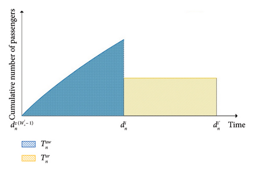
In the urban rail transit system, due to the high departure frequency, the passenger flow can be processed as a cumulative curve related to the time interval [47]. The waiting time of passengers waiting for the first train after arriving at the station can be approximately calculated as the uniform arrival, which can be illustrated as the blue part of Figure 6.
Hence, the arrival waiting time can be formulated as equation (9):
()
Passengers waiting for subsequent trains can be divided into two scenarios. One scenario is that due to the remaining capacity constraints of the train, passengers are unable to board the current train and need to wait for subsequent trains. Another scenario is that due to the inability of the previous train to reach the destination directly, passengers actively choose to wait for the subsequent train. The waiting time for a single passenger is equal to the departure interval between two trains, which can be illustrated as the yellow part of Figure 6. The waiting time for subsequent trains can be formulated as equation (10):
()
Thus, the waiting time can be stated as equation (11):
()
2.
In-Vehicle Travel Time
As shown in equation (12), the in-vehicle travel time consists of the running time in the interval and the dwelling time at the station:
()
3.
Transfer Time
The transfer time consists of two parts: the transfer walking time and the transfer waiting time. As the fact that passengers can transfer between skip-stop trains and all-stop trains at the same platform, the transfer walking time can be ignored. Therefore, as shown in equation (13), when passengers transfer from train i at station n to train i^∗, the transfer waiting time is equal to the departure interval between train i and train i^∗ at station n:
()
where indicates the number of passengers transferring from train i to train i^∗ at station n.

4.4. Constraints

1.
Constraints on Train Dwell Time at Stations
The train dwell time should be longer than the minimum value, which is formulated as follows:
()
where is the minimum dwell time.
2.
Constraints on Interval Running Time
The running time of a train in a section should not be less than the minimum running time. The constraint can be written as formula (15). Formula (16) indicates the calculation method for the minimum running time between two stations, which is calculated from the pure running time and additional acceleration and deceleration time, i.e., t_acc and t_dec, due to the stop:
()

()
3.
Constraints on Safety Headway
Formulas (17)–(21) ensure that the headways of trains are not below the minimum safety headway. Considering the overtaking between trains, the constraints find the train number through the departure sequence and the function z(∗) defined in 4.2, ensuring the safety of independent trains that arrive sequentially in occupied sections.
Formulas (17)–(20) consider that two trains within a virtual coupled train should have the same arrival and departure times in the section that operates as a virtual coupled train. Formula (21) constrains the headway of trains based on whether the train is overtaking or being overtaken by other trains at the station:
()

()

()

()

()
where and indicate whether the trains arrive at or depart from the station in a virtual coupled state.
4.
Constraints on Study Period
The arrival and departure times of trains at the station should be within the study period, and the constraints are shown in formulas (22) and (23):
()

()
where is the start time of the study period and is the end time of the study period.
5.
Constraints on Virtual Operations
As shown in formulas (24)–(29), only when both trains stop at the station can virtual operations be carried out at that station:
()

()

()

()

()

()

Considering that the same train can operate virtual coupling and decoupling at most once during operation. And the same pair of trains can only operate virtual coupling or decoupling at the same station at most. The constraints are shown in formulas (30)–(33):

()

In the section where the train operates as a virtual coupled train, the stopping patterns of the two trains inside the virtual coupled train should be the same. The constraints also need to be set as formula (34):

()

where n^∗1 and n^∗2 indicate the stations where the trains operate virtual coupling and virtual decoupling, respectively.

The state of trains when they arrive and depart from the station is related to whether the trains operate virtual coupling or decoupling at the station. This constraint can be indicated as formula (35):

()

5. Solution Algorithms

The optimization model for a skip-stop timetable under the application of virtual coupling technology proposed in this paper has multiple and complex constraints. The ALNS algorithm is a problem-solving method that utilizes multiple pairs of destroy operators and repair operators to reconstruct the current solution, dynamically adjusting the weight of the operators and finding the optimal solution faster and better [45]. The procedure can be controlled by the SA algorithm, and its core idea (i.e. the metropolis criterion) can prevent the algorithm from falling into local optima. In this study, a hybrid algorithm was designed to solve the model. The algorithm steps are shown in Table 3.

Table 3. Hybrid algorithm steps.

Specific operation

Step 1: Initialization

Step 2: Randomly generate the initial solution (initialize the train timetable and overtaking location) and calculate the objective function value f(x). Let x^best⟵x, f(x^best)⟵f(x), heating number reheat⟵0, and iteration number iter⟵0. Set the initial temperature T₀, termination temperature T_end, the weights ω_i, and scores β_i of the combination operators, and the maximum value iter_max of iterations

Step 3: If the heating frequency reheat is less than 20, proceed to step 4; otherwise, proceed to step 12

Step 4: Set the current temperature value t⟵T₀

Step 5: If the current temperature t > T_end and iteration number iter < iter_max, proceed to step 6; otherwise, proceed to step 11

Step 6: Randomly select a combination operator based on the weights using roulette wheel to reconstruct the current solution and obtain a new solution x^t. Update the objective function value f(x^t) and the number of times the operator n_o,i

Step 7: According to the value f(x^t), update the score β_i of the combination operator and the optimal value f(x^best) of the objective function according to the Metropolis criterion

Step 8: If the current iteration has completed a stage (iter is an integer multiple of γ), proceed to step 9; otherwise, proceed to step 10

Step 9: Update the weights ω_i of the combination operators and reset the scores β_i of the combination operators.

Step 10: Update the current temperature t⟵v × t and iteration number iter⟵iter + 1 and proceed to step 5

Step 11: Update heating frequency reheat⟵reheat + 1 and proceed to step 3

Step 12: Output f(x^best) and end the algorithm

5.1. Initial Solution

The initial solution of the algorithm is a feasible solution randomly generated according to certain rules. Firstly, the departure times of a certain number of different types of trains are randomly generated during the research period and the initial timetable is obtained based on the stopping plan, interval running time, etc. This timetable may have some conflicts due to the different travel speeds of different trains. Based on the conflicts in the timetable and the location of the overtaking station, the overtaking between trains at the station can be set. Finally, overall adjustments to the timetable are made to generate an initial feasible solution that includes overtaking.

5.2. List of Operators

The destroy and repair operators are combined to form four sets of combination operators. There are two sets of station selection operators, each consisting of coupling operators and decoupling operators. The station selection operator selects the station for virtual coupling and decoupling operations. The other two sets are train operators, consisting of train insert and remove operators. The detailed description of the operator is as follows.

5.2.1. Station Selection Operators

1.
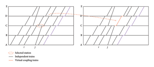
Station Selection Operator 1 Station selection operator 2 selects continuous trains and stations for virtual operations randomly, where both trains need to stop at the station. The coupling operator randomly selects a station (represented by N) as the station where two vehicles operate the virtual coupling. The decoupling operator selects a station from the stations where two trains stop continuously and simultaneously after station N, as the station where the two trains operate virtual decoupling. As shown in Figure 7, there are stations A, C, D, and E where both train i and train j stop. The coupling operator randomly selects station C to make two trains operate virtual coupling. The decoupling operator randomly selects station D as the station for virtual decoupling operation. The virtual operation of trains i and j can be described as two trains operating virtual coupling at station C and becoming a coupled train running to station D. The two trains operate virtual decoupling at station D and are restored to two independent trains running separately.
2.
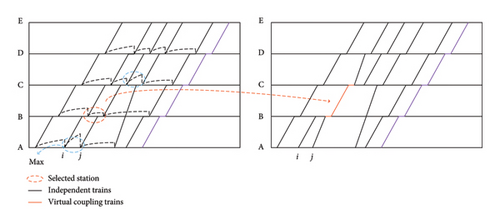
Station Selection Operator 2 Station selection operator 2 selects stations based on passenger demand, which require both trains to stop. The coupling operator searches for the station after the interval with the largest passenger demand. Select a station (represented by N) in the rear that is closest to the station and both trains, which are immediately adjacent to that interval and are parked as the location for operating virtual coupling. The decoupling operator searches for the interval with the largest passenger demand after the second train, making the two trains operate virtual decoupling at the station where the interval is located. It should be noted that the selection of stations is similar to station selection operator 1, which is a station where two consecutive trains stop at the same time after station N, as shown in Figure 8.

5.2.2. Train Operators

1.
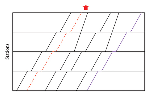
Train Operator 1 Train operator 1 selects trains that are inserted and removed randomly. The train remove operator removes a train randomly, while the train insert operator inserts a train randomly, as shown in Figure 9.
2.
Train operator 2 selects the inserted and removed trains based on the passenger flow demand in the interval. The train remove operator removes a train with the lowest passenger demand, while the train insert operator inserts a train in the interval with the largest passenger demand, as shown in Figure 10.

5.2.3. Some Details

1.
When the solution is reconstructed through operators, the departure and arrival times of trains may be adjusted due to the constraints of safe headway. The overtaking and virtual coupling between trains can create connections between them. When making adjustments to these trains, it is important to note whether only one train needs to be adjusted or whether other related trains need to be adjusted simultaneously.
2.
When inserting a train through a train operator, the train cannot be inserted between trains that have undergone overtaking or virtual coupling. The inserted train needs to stop at the station where the interval is located. If more than one type of train stops at that station, the type of inserted train is different from the type of train before the interval. If the position of the inserted train is before the first train, insert an all-stop train.
3.
After inserting a new train through the train operator each time, it can be determined whether the train can overtake another train or be overtaken by another train, and the overtaking operation can be performed.
4.
If it is not possible to operate the station selection operator or train operator at the interval with the highest passenger demand, then choose the interval with the second highest passenger demand, and so on.

5.3. Metropolis Criterion

The metropolis criterion causes the algorithm to accept a deteriorating solution with a certain probability p, which is calculated as shown in equation (36):

()

where f(x) is the objective function value of the initial solution, f(x^t) is the objective function value of the current solution, and t is the current temperature. For the random number r between [0,1), if p ≥ r, the current solution is accepted as the initial solution for the next iteration; otherwise, the current solution is rejected.

5.4. Update of Operator Weights

According to Barrena et al. [46], the weight of the combination operator can be calculated using the following equation:

()

where ω_i is the weight of the combination operator, and β_i is the score of the combination operator. n_o,i is the number of times the combination operator is executed in stage o, with γ iterations per stage. There are four optimization effects of the current solution during the iteration process:

1.
The current solution is not feasible.
2.
The current solution is feasible and superior to the optimal solution.
3.
The current solution is feasible and superior to the initial solution.
4.
The current solution is feasible and not superior to the initial solution, but meets the metropolis criterion.

The corresponding combination operator score is updated based on the optimization effect of the current solution. The higher the combination operator score, the greater the operator weight, and the greater the probability of being selected.

6. Case Study

6.1. Case Introduction

A certain urban rail transit line R is a skip-stop-operated urban rail transit line that connects the urban and suburban areas of the city. The total mileage of the line is about 60.6km, with a total of 21 stations, of which stations 7, 10, 12, 15, 18, and 19 are overtaking stations. The maximum operating speed of the line design is 120km/h. The stopping plan of skip-stop trains on the R line is shown in Table 4, and the spatiotemporal distribution of the passenger flow on the R line is illustrated in Figure 11.

Table 4. Train stopping plan.

Station number	Skip-stop train stop plan (equals 1 if the train stops and 0 otherwise)
1	1
2	1
3	1
4	1
5	0
6	1
7	1
8	0
9	1
10	0
11	0
12	0
13	0
14	1
15	0
16	0
17	1
18	0
19	0
20	0
21	1

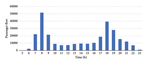
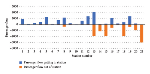
The mileage and interval distance of line R are relatively large, with the initial and final stations located in the central urban area and suburban areas, respectively. The service range of the line is relatively large, and the distribution of the passenger flow shows a significant temporal and spatial imbalance. The passenger flow demand of line R exhibits a clear bimodal distribution throughout the day, with the morning peak occurring from 7:00 to 9:00 and the evening peak occurring from 17:00 to 19:00 (see Figure 11(a)). During the morning peak hours of line R, the number of passengers arriving and departing the station is relatively small at stations 1–11, with more at stations 12–21. Among them, passengers departing the station are concentrated at stations 13–21 (see Figure 11(b)).

6.2. Passenger Demand and Parameter Setting

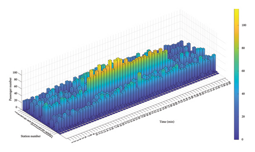
The study selected the morning peak period (8:00–8:59) in the upstream direction of a certain working day for research, during which a total of 25,125 passengers took the train. The distribution of passengers arriving at each station is shown in Figure 12, with blue indicating fewer passengers and yellow indicating more passengers. From the graph, it can be seen that during peak hours, the arrival of passengers at each station shows a pattern of more concentration in the middle period (20–40 min) and a decrease at both ends (0–20 and 40–60 min).

Regardless of specific line conditions, the study assumes that the fastest operating mode for a train in a section is as follows: the train accelerates uniformly to the maximum operating speed of the section with maximum acceleration after departing from the station, then advances at a constant speed until it needs to stop at the station with maximum deceleration, and the train stops steadily when the speed is 0. The shortest time for all-stop train and skip-stop train to operate in the section is calculated based on their stopping plan, as shown in Table 5.

Table 5. Line R interval length and interval running time.

Interval number	Station spacing (km)	Pure running time (min)	Additional time of train acceleration (min)	Additional time of train deceleration (min)	The shortest running time of all-stop train (min)	The shortest running time of skip-stop train (min)
1	1.2	1.2	0.1	0.3	1.3	1.3
2	3.3	2.9	0.2	0.4	2.3	2.3
3	2.1	1.8	0.2	0.3	1.7	1.7
4	1.2	1.2	0.1	0.2	1.3	0.9
5	2.1	1.6	0.2	0.3	1.7	1.4
6	3.4	3.0	0.2	0.3	2.4	2.4
7	1.9	1.6	0.2	0.4	1.6	1.3
8	2.5	2.1	0.1	0.3	1.9	1.6
9	2.2	2.0	0.1	0.4	1.8	1.4
10	3	2.2	0.2	0.5	2.2	1.5
11	6.1	4.2	0.1	0.4	3.7	3.1
12	6.1	4.3	0.2	0.3	3.7	3.1
13	2.2	1.8	0.1	0.3	1.8	1.4
14	2.1	1.7	0.1	0.4	1.7	1.4
15	3.2	2.7	0.2	0.3	2.3	1.6
16	2.9	2.1	0.2	0.3	2.1	1.8
17	3.2	2.4	0.1	0.3	2.3	1.9
18	4.5	3.2	0.1	0.3	2.9	2.3
19	5	3.4	0.1	0.4	3.2	2.5
20	2.4	2.1	0.1	0.3	1.9	1.5

To ensure safety, the longest dwell time at the station is used to calculate the headway. The interval running time of the train is taken as 120km/h. To facilitate the design and calculation of the timetable, the headway of trains under the CBTC system is taken as 2 min, and the headway of trains under the application of virtual coupling technology is 1.8 min, while the headway of trains with multiple formation is 2 min.

According to the actual situation of the line operation, there are approximately 13 trains operating between 8:00 and 9:00 during the morning peak hours, with the capacity of a train taken as 1962. Therefore, it is assumed that the operating frequency of trains during the study period is 13 trains per hour.

In Table 6, the relevant parameters of the adaptive neighborhood search algorithm used in the case study are listed.

Table 6. Parameters related to adaptive neighborhood search algorithm.

Parameters	Value
Initial temperature T₀	100,000
Termination temperature T_end	0.01
Cooling rate v
Maximum number of iterations iter_max	200,000

6.3. Results

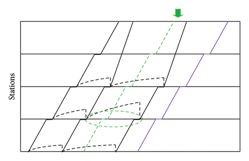
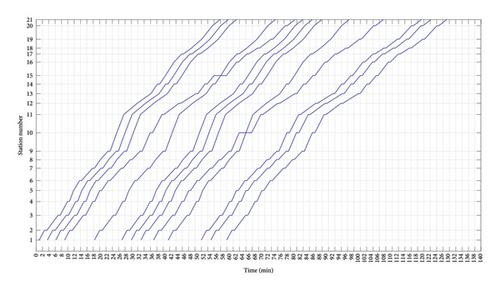
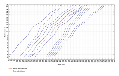
According to the different communication technologies used and whether the timetable has been optimized, the timetables are divided into Scheme 1, Scheme 2, and Scheme 3, as shown in Figure 13, 14, and 15. Scheme 1 and Scheme 2 are randomly generated initial timetables, with Scheme 1 applying traditional technology and Scheme 2 applying virtual coupling technology. There are no changes in train types and departure sequences between the two schemes, only some differences in tracking intervals. Scheme 3 is an optimized timetable, with Scheme 2 as the initial solution, which is optimized through the algorithm proposed in the previous chapters. The communication technology it applies is virtual coupling technology.

The variation of the objective function value (i.e. the total travel time of passengers) decreases periodically with the number of iterations during the optimization process from Scheme 2 to Scheme 3. In the early stages of the iteration (i.e., the first 1500 iterations), the objective function value rapidly decreases, then periodically decreases as the number of iterations continues to increase, and eventually stabilizes around 3200 iterations. The total travel time of passengers for different schemes is shown in Table 7. From the table, it can be seen that the optimized timetable (i.e. Scheme 3) applying virtual coupling technology has a certain improvement in the total travel time of passengers compared to the other two schemes.

Table 7. Comparison of passengers’ travel times for different schemes.

	Scheme 1	Scheme 2	Scheme 3
Total travel time (min)	657,716.3	657,034.9	608,988.8
Optimization effect	7.4%	7.3%	—

There is a crossover in the initial solution of applying two communication technologies separately. Under traditional CBTC conditions, all-stop train waits for skip-stop train at the overtaking station for 4 min, while this time is reduced to 3.6 min by 10% applying virtual coupling technology. This has shortened the on-board time of some passengers, especially those waiting for skip-stop train to overtake all-stop train, by about 12.4%, thereby shortening the total travel time of passengers by about 9.6%.

Table 8 shows the changes in the passengers’ travel time after the algorithm optimization of Scheme 2 to Scheme 3 under the same communication technology application. From the table, it can be concluded that Scheme 3 has been optimized for Scheme 2 in various components of the passengers’ travel time, with the highest proportion of optimization being the waiting time for subsequent trains and the transfer time, which are optimized by 65.9% and 57.0%, respectively. The waiting time for arrival passengers is reduced by about 300 min, with an optimization effect of about 0.3%. The in-vehicle travel time is shortened by about 5102 min, and the optimization effect is about 1.0%.

Table 8. Composition of passengers’ travel time between Scheme 2 and Scheme 3.

	Total travel time	Waiting time for arrival passengers	In-vehicle travel time	Waiting time for subsequent trains	Transfer time
Scheme 2 (min)	657,034.9	90,307.3	494,299.2	15,435.2	56,993.2
Scheme 3 (min)	608,988.8	90,006.7	489,196.9	5258.5	24,526.7
Optimize proportion	7.3%	0.3%	1.0%	65.9%	57.0%

As shown in Table 9, compared with Scheme 1, the total running time of trains in Scheme 2 is reduced by adjusting the train tracking interval. One of the reasons is the shortened train tracking interval, which shortens the time for the all-stop train to wait for skip-stop train to overtake. Based on passenger demand, the operating ratio of skip-stop train to all-stop train is changed from 8:5 to 4:9 in the optimized timetable, which is more in line with the actual situation.

Table 9. Trains’ running time and optimization effect of different schemes.

		Scheme 1	Scheme 2	Scheme 3
Skip-stop train	Train quantity	8	8	4
	Average operating time (min)	56.9	56.9	56.9
	Proportion of changes in the operating time	0%	0%	—

All-stop train	Train quantity	5	5	9
	Average operating time (min)	70.6	70.5	69.8
	Proportion of changes in the operating time	−1.1%	−0.9%	—

Total operating time (min)		808.4	807.6	856.2

7. Conclusions

In this paper, we focused on the optimization of skip-stop train schedules in urban rail transit under the application of virtual coupling technology. The calculation method for the tracking interval of urban rail transit trains at stations under the application of virtual coupling technology has been studied and sorted out, which provides a theoretical basis for the engineering application of virtual coupling technology. The optimization model for skip-stop train schedules of virtual coupling trains has been constructed. The model aims to minimize the total travel time of passengers, focuses on the change of train sequence caused by overtaking between trains, and sets the basic constraints such as dwell time constraints, interval running time constraints, and safe headway constraints. Based on the differences between virtual coupling trains and traditional trains, constraints on virtual operations are designed, including the selection of locations for virtual operations and the relationship between virtual operations and the arrival and departure status of trains. A hybrid algorithm is designed to solve the model. A case of a certain urban rail transit line R showed that the optimized timetable can effectively reduce the total travel time of passengers, and the model and algorithm are effective in practical applications.

Future research can focus on the following aspects: (1) The calculation method for the tracking interval of urban rail transit trains will be studied, which can pay more attention to the operational status of trains during the actual operation, by paying attention to the train speed curve or using simulation to conduct in-depth research. (2) The relationship between passenger demand and virtual coupling application technology, as well as passengers’ choice behavior, deserves further research. (3) The problem of bidirectional lines and complex networks is more complex and practical, and the problem of train turnover applying virtual coupling technology is also worth in-depth research.

Conflicts of Interest

The authors declare no conflicts of interest.

Funding

This study was supported by the Fundamental Research Funds for the Central Universities (No. 2022JBMC058) and Beijing Natural Science Foundation (No. L201013).

Acknowledgments

This study was supported by the Fundamental Research Funds for the Central Universities (No. 2022JBMC058) and Beijing Natural Science Foundation (No. L201013).

Open Research

Data Availability Statement

The data used to support the findings of this study are available from the corresponding author upon request.

References

1 Zhou Q. R., Analysis of the Express/Slow Trains Operation Mode for Urban Rail Transit of World Cities, Urban Rapid Rail Transit. (2013) 26, no. 2, 18–22.
Google Scholar
2 Abdelhafiez E. A., Salama M. R., and Shalaby M. A., Minimizing Passenger Travel Time in URT System Adopting Skip-Stop Strategy, Journal of Rail Transport Planning & Management. (2017) 7, no. 4, 277–290, https://doi.org/10.1016/j.jrtpm.2017.11.001, 2-s2.0-85035150370.
10.1016/j.jrtpm.2017.11.001
Google Scholar
3 Gu W., Amini Z., and Cassidy M. J., Exploring Alternative Service Schemes for Busy Transit Corridors, Transportation Research Part B: Methodological. (2016) 93, 126–145, https://doi.org/10.1016/j.trb.2016.07.010, 2-s2.0-84994417607.
10.1016/j.trb.2016.07.010
Web of Science® Google Scholar
4 Jiang F., Cacchiani V., and Toth P., Train Timetabling by Skip-Stop Planning in Highly Congested Lines, Transportation Research Part B: Methodological. (2017) 104, 149–174, https://doi.org/10.1016/j.trb.2017.06.018, 2-s2.0-85021840373.
10.1016/j.trb.2017.06.018
Web of Science® Google Scholar
5 Zolfaghari S., Azizi N., and Jaber M. Y., A Model for Holding Strategy in Public Transit Systems with Real-Time Information, International Journal of Transport Management. (2004) 2, no. 2, 99–110, https://doi.org/10.1016/j.ijtm.2005.02.001, 2-s2.0-33747384609.
10.1016/j.ijtm.2005.02.001
Google Scholar
6 Bock U. and Bikker G., Design and Development of a Future Freight Train Concept-Virtually Coupled Train Formations, IFAC Proceedings Volumes. (2000) 33, no. 9, 395–400, https://doi.org/10.1016/s1474-6670(17)38176-4.
10.1016/S1474-6670(17)38176-4
Google Scholar
7 Konig S. and Schnieder E., Modeling and Simulation of an Operation Concept for Future Rail Traffic, Proceedings of the 2001 IEEE Intelligent Transportation Systems Conference (ITSC), August 2001.
Google Scholar
8 Ständer D. I. T., Drewes J., Braun I., and Schnieder E., Operational and Safety Concepts for Railway Operation with Virtual Train-Sets, IFAC Proceedings Volumes. (2006) 39, no. 12, 261–266, https://doi.org/10.3182/20060829-3-nl-2908.00046.
10.3182/20060829-3-NL-2908.00046
Google Scholar
9 Flammini F., Marrone S., Nardone R., Petrillo A., Santini S., and Vittorini V., Towards Railway Virtual Coupling, Proceedings of the 2018 IEEE International Conference on Electrical Systems for Aircraft, Railway, Ship Propulsion and Road Vehicles & International Transportation Electrification Conference (ESARS-ITEC), November 2018.
Google Scholar
10 Aoun J., Quaglietta E., and Goverde R., Exploring Demand Trends and Operational Scenarios for Virtual Coupling Railway Signalling Technology, Proceedings of the 2020 IEEE 23rd International Conference on Intelligent Transportation Systems (ITSC), September 2020.
Google Scholar
11 Meo C. D., Vaio M. D., Flammini F., Nardone R., Santini S., and Vittorini V., ERTMS/ETCS Virtual Coupling: Proof of Concept and Numerical Analysis, IEEE Transactions on Intelligent Transportation Systems. (2019) 21, no. 6, 2545–2556.
10.1109/TITS.2019.2920290
Web of Science® Google Scholar
12 Lichtblau J., Scheiner B., Michler F. et al., Novel Approach for Virtual Coupling of Trains Using Different Modulation and Coding Schemes, Proceedings of the 2018 International Conference on Intelligent Rail Transportation (ICIRT), December 2018.
Google Scholar
13 Felez J. and Vaquero-Serrano M. A., Virtual Coupling in Railways: A Comprehensive Review, Machines. (2023) 11, no. 5, https://doi.org/10.3390/machines11050521.
10.3390/machines11050521
Web of Science® Google Scholar
14 Cao Y., Ma L. C., Xiao S., Zhang X., and Xu W., Standard Analysis for Transfer Delay in CTCS-3, Chinese Journal of Electronics. (2017) 26, no. 5, 1057–1063, https://doi.org/10.1049/cje.2017.08.024, 2-s2.0-85029353186.
10.1049/cje.2017.08.024
Web of Science® Google Scholar
15 Zhang Y. Z., Cao Y., Wen Y. H., Liang L., and Zou F., Optimization of Information Interaction Protocols in Cooperative Vehicle-Infrastructure Systems, Chinese Journal of Electronics. (2018) 27, no. 2, 439–444, https://doi.org/10.1049/cje.2017.10.009, 2-s2.0-85048807089.
10.1049/cje.2017.10.009
Web of Science® Google Scholar
16 Cao Y., Li P., and Zhang Y. Z., Parallel Processing Algorithm for Railway Signal Fault Diagnosis Data Based on Cloud Computing, Future Generation Computer Systems. (2018) 88, 279–283, https://doi.org/10.1016/j.future.2018.05.038, 2-s2.0-85048592068.
10.1016/j.future.2018.05.038
Web of Science® Google Scholar
17 Felez J., Kim Y., and Borrelli F., A Model Predictive Control Approach for Virtual Coupling in Railways, IEEE Transactions on Intelligent Transportation Systems. (2019) 20, no. 7, 2728–2739, https://doi.org/10.1109/tits.2019.2914910, 2-s2.0-85068269132.
10.1109/TITS.2019.2914910
Web of Science® Google Scholar
18 Liu L., Wang P., Zhang B., and Wei W., Coordinated Control Method of Virtually Coupled Train Formation Based on Multi Agent System, Proceedings of the Second International Conference on Smart Vehicular Technology, Transportation, Communication and Applications, October 2018.
Google Scholar
19 Liu L., Research and Prospect of Intelligent Control Technology for Virtually Coupled Train Formation, Railway Signalling & Communication Engineering. (2020) 17, no. 2, 1–9.
Google Scholar
20 Park J., Lee B. H., and Eun Y., Virtual Coupling of Railway Vehicles: Gap Reference for Merge and Separation, Robust Control, and Position Measurement, IEEE Transactions on Intelligent Transportation Systems. (2022) 23, no. 2, 1085–1096, https://doi.org/10.1109/tits.2020.3019979.
10.1109/TITS.2020.3019979
Web of Science® Google Scholar
21 Quaglietta E., Wang M., and Goverde R., A Multi-State Train-Following Model for the Analysis of Virtual Coupling Railway Operations, Journal of Rail Transport Planning & Management. (2020) 15, https://doi.org/10.1016/j.jrtpm.2020.100195.
10.1016/j.jrtpm.2020.100195
Web of Science® Google Scholar
22 Luo X. L., Tang T., Liu H. J., Zhang L., and Li K. C., An Adaptive Model Predictive Control System for Virtual Coupling in Metros, Actuators. (2021) 10, no. 8, https://doi.org/10.3390/act10080178.
10.3390/act10080178
Web of Science® Google Scholar
23 Cao Y., Wen J. K., and Ma L. C., Tracking and Collision Avoidance of Virtual Coupling Train Control System, Future Generation Computer Systems. (2021) 120, 76–90, https://doi.org/10.1016/j.future.2021.02.014.
10.1016/j.future.2021.02.014
Web of Science® Google Scholar
24 Wang H. W., Zhao Q. Q., Lin S. Y. et al., A Reinforcement Learning Empowered Cooperative Control Approach for IIoT-Based Virtually Coupled Train Sets, IEEE Transactions on Industrial Informatics. (2021) 17, no. 7, 4935–4945, https://doi.org/10.1109/tii.2020.3024946.
10.1109/TII.2020.3024946
Web of Science® Google Scholar
25 Liu H., Luo X., Tang T., Zhang Y., and Chai M., A Hierarchical Control Approach for Virtual Coupling in Metro Trains, Computer-Aided Civil and Infrastructure Engineering. (2024) 39, no. 9, 1318–1336, https://doi.org/10.1111/mice.13138.
10.1111/mice.13138
Web of Science® Google Scholar
26 Su H. X., Chai M., Chen L. J., and Lv J. D., Deep Learning-Based Model Predictive Control for Virtual Coupling Railways Operation, Proceedings of the 2021 IEEE International Intelligent Transportation Systems Conference (ITSC), September 2021.
Google Scholar
27 Chai M., Su H. X., and Liu H. J., Long Short-Term Memory-Based Model Predictive Control for Virtual Coupling in Railways, Wireless Communications and Mobile Computing. (2022) 2022, 1–17, https://doi.org/10.1155/2022/1859709.
10.1155/2022/1859709
Google Scholar
28 D3.1 Virtual Coupling Communication Solutions analysis[EB/OL], 2018.
Google Scholar
29 Ma S. M., Bu B., and Wang H. W., A Virtual Coupling Approach Based on Event-Triggering Control for CBTC Systems under Jamming Attacks, Proceedings of the 2020 IEEE 92nd Vehicular Technology Conference (VTC2020-Fall), December 2020, Canada.
Google Scholar
30 Cao Y., Wen J. K., and Ma L. C., Dynamic Marshalling and Scheduling of Trains in Major Epidemics, Journal of Traffic and Transportation Engineering. (2020) 20, no. 3, 120–128.
Google Scholar
31 Lee B. H., Chae S. Y., and Choi H. Y., Skip and Stop Scheduling Based on Virtually Coupled Trains, Journal of the Korean Society for Railway. (2020) 23, no. 1, 80–88, https://doi.org/10.7782/jksr.2020.23.1.80.
10.7782/JKSR.2020.23.1.80
Google Scholar
32 Gallo F., Febbraro A. D., Giglio D., and Sacco N., A Mathematical Programming Model for the Management of Carriages in Virtually Coupled Trains, Proceedings of the 2020 IEEE 23rd International Conference on Intelligent Transportation Systems (ITSC), Rhodes, Greece, September 2020.
Google Scholar
33 Muniandi G., Blockchain-enabled Virtual Coupling of Automatic Train Operation Fitted Mainline Trains for Railway Traffic Conflict Control, IET Intelligent Transport Systems. (2020) 14, no. 6, 611–619, https://doi.org/10.1049/iet-its.2019.0694.
10.1049/iet-its.2019.0694
Web of Science® Google Scholar
34 Gallo F., Febbraro A. D., Giglio D., and Sacco N., Planning and Optimization of Passenger Railway Services with Virtually Coupled Trains, Proceedings of the 2021 7th International Conference on Models and Technologies for Intelligent Transportation Systems (MT-ITS), Heraklion, Greece, June 2021.
Google Scholar
35 You T. and Yang Z., Optimal Design of Urban Rail Train Operation Plan Based on Virtual Coupling, Proceedings of the 2021 3rd International Academic Exchange Conference on Science and Technology Innovation (IAECST), December 2021.
Google Scholar
36 Chen C., Zhu L., and Wang X., An Integrated Train Scheduling Optimization Approach for Virtual Coupling Trains, 2022 IEEE 25th International Conference on Intelligent Transportation Systems (ITSC), Macau, China, October 2022.
Google Scholar
37 Zhang J., Simulation-based Schedule Optimization for Virtual Coupling-Enabled Rail Transit Services with Multiagent Technique, Journal of Advanced Transportation. (2023) 2023, https://doi.org/10.1155/2023/3196066.
10.1155/2023/3196066
Web of Science® Google Scholar
38 Zhang J., Exploring the Intra-platoon Planning Problem for Heterogeneous Train Traffic under Virtual Coupling in the Railway Network via Simulation, Journal of Rail Transport Planning & Management. (2024) 30, https://doi.org/10.1016/j.jrtpm.2024.100442.
10.1016/j.jrtpm.2024.100442
Web of Science® Google Scholar
39 Park Y. and Ha H. K., Analysis of the Impact of High-Speed Railroad Service on Air Transport Demand, Transportation Research Part E: Logistics and Transportation Review. (2006) 42, no. 2, 95–104, https://doi.org/10.1016/j.tre.2005.09.003, 2-s2.0-30044444801.
10.1016/j.tre.2005.09.003
Web of Science® Google Scholar
40 Román C. and Martín J. C., Integration of HSR and Air Transport: Understanding Passengers’ Preferences, Transportation Research Part E: Logistics and Transportation Review. (2014) 71, 129–141, https://doi.org/10.1016/j.tre.2014.09.001, 2-s2.0-84908173828.
10.1016/j.tre.2014.09.001
Web of Science® Google Scholar
41 Li Z. C. and Sheng D., Forecasting Passenger Travel Demand for Air and High-Speed Rail Integration Service: A Case Study of Beijing-Guangzhou Corridor, China, Transportation Research Part A: Policy and Practice. (2016) 94, 397–410, https://doi.org/10.1016/j.tra.2016.10.002, 2-s2.0-84991730363.
10.1016/j.tra.2016.10.002
Web of Science® Google Scholar
42 Yin J. T., Yang L. X., Tang T., Gao Z. Y., and Ran B., Dynamic Passenger Demand Oriented Metro Train Scheduling with Energy-Efficiency and Waiting Time Minimization: Mixed-Integer Linear Programming Approaches, Transportation Research Part B: Methodological. (2017) 97, 182–213, https://doi.org/10.1016/j.trb.2017.01.001, 2-s2.0-85009124442.
10.1016/j.trb.2017.01.001
Web of Science® Google Scholar
43 Dong X. L., Li D. W., Yin Y. H., Ding S. S., and Cao Z. C., Integrated Optimization of Train Stop Planning and Timetabling for Commuter Railways with an Extended Adaptive Large Neighborhood Search Metaheuristic Approach, Transportation Research Part C: Emerging Technologies. (2020) 117, https://doi.org/10.1016/j.trc.2020.102681.
10.1016/j.trc.2020.102681
Web of Science® Google Scholar
44 Zhang T., Li D., and Qiao Y., Comprehensive Optimization of Urban Rail Transit Timetable by Minimizing Total Travel Times under Time-dependent Passenger Demand and Congested Conditions, Applied Mathematical Modelling. (2018) 58, 421–446, https://doi.org/10.1016/j.apm.2018.02.013, 2-s2.0-85043990747.
10.1016/j.apm.2018.02.013
Web of Science® Google Scholar
45 Ropke S. and Pisinger D., An Adaptive Large Neighborhood Search Heuristic for the Pickup and Delivery Problem with Time Windows, Transportation Science. (2006) 40, no. 4, 455–472, https://doi.org/10.1287/trsc.1050.0135, 2-s2.0-33751011598.
10.1287/trsc.1050.0135
Web of Science® Google Scholar
46 Barrena E., Canca D., Coelho L. C., and Laporte G., Exact Formulations and Algorithm for the Train Timetabling Problem with Dynamic Demand, Computers & Operations Research. (2014) 44, 66–74, https://doi.org/10.1016/j.cor.2013.11.003, 2-s2.0-84888192388.
10.1016/j.cor.2013.11.003
Web of Science® Google Scholar

Citing Literature

All articles

Interval number	Station spacing (km)	Pure running time (min)	Additional time of train acceleration (min)	Additional time of train deceleration (min)	The shortest running time of all-stop train (min)	The shortest running time of skip-stop train (min)
1	1.2	1.2	0.1	0.3	1.3	1.3
2	3.3	2.9	0.2	0.4	2.3	2.3
3	2.1	1.8	0.2	0.3	1.7	1.7
4	1.2	1.2	0.1	0.2	1.3	0.9
5	2.1	1.6	0.2	0.3	1.7	1.4
6	3.4	3.0	0.2	0.3	2.4	2.4
7	1.9	1.6	0.2	0.4	1.6	1.3
8	2.5	2.1	0.1	0.3	1.9	1.6
9	2.2	2.0	0.1	0.4	1.8	1.4
10	3	2.2	0.2	0.5	2.2	1.5
11	6.1	4.2	0.1	0.4	3.7	3.1
12	6.1	4.3	0.2	0.3	3.7	3.1
13	2.2	1.8	0.1	0.3	1.8	1.4
14	2.1	1.7	0.1	0.4	1.7	1.4
15	3.2	2.7	0.2	0.3	2.3	1.6
16	2.9	2.1	0.2	0.3	2.1	1.8
17	3.2	2.4	0.1	0.3	2.3	1.9
18	4.5	3.2	0.1	0.3	2.9	2.3
19	5	3.4	0.1	0.4	3.2	2.5
20	2.4	2.1	0.1	0.3	1.9	1.5

Interval number	Station spacing (km)	Pure running time (min)	Additional time of train acceleration (min)	Additional time of train deceleration (min)	The shortest running time of all-stop train (min)	The shortest running time of skip-stop train (min)
1	1.2	1.2	0.1	0.3	1.3	1.3
2	3.3	2.9	0.2	0.4	2.3	2.3
3	2.1	1.8	0.2	0.3	1.7	1.7
4	1.2	1.2	0.1	0.2	1.3	0.9
5	2.1	1.6	0.2	0.3	1.7	1.4
6	3.4	3.0	0.2	0.3	2.4	2.4
7	1.9	1.6	0.2	0.4	1.6	1.3
8	2.5	2.1	0.1	0.3	1.9	1.6
9	2.2	2.0	0.1	0.4	1.8	1.4
10	3	2.2	0.2	0.5	2.2	1.5
11	6.1	4.2	0.1	0.4	3.7	3.1
12	6.1	4.3	0.2	0.3	3.7	3.1
13	2.2	1.8	0.1	0.3	1.8	1.4
14	2.1	1.7	0.1	0.4	1.7	1.4
15	3.2	2.7	0.2	0.3	2.3	1.6
16	2.9	2.1	0.2	0.3	2.1	1.8
17	3.2	2.4	0.1	0.3	2.3	1.9
18	4.5	3.2	0.1	0.3	2.9	2.3
19	5	3.4	0.1	0.4	3.2	2.5
20	2.4	2.1	0.1	0.3	1.9	1.5

Optimization of Skip-Stop Train Schedule in Urban Rail Transit Under Virtual Coupling

Abstract

1. Introduction

2. Literature Review

2.1. Train Operation Control and Communication Technology

2.2. Transportation Organization

3. Analysis of Skip-Stop Operation Using Virtual Coupling Technology

4. Mathematical Modeling

4.1. Problem Statement

4.1.1. Passenger Choice Behavior

4.1.2. Definition of the Research Question

4.2. Passenger Parameter Description

4.3. Objective Functions

4.4. Constraints

5. Solution Algorithms

5.1. Initial Solution

5.2. List of Operators

5.2.1. Station Selection Operators

5.2.2. Train Operators

5.2.3. Some Details

5.3. Metropolis Criterion

5.4. Update of Operator Weights

6. Case Study

6.1. Case Introduction

6.2. Passenger Demand and Parameter Setting

6.3. Results

7. Conclusions

Conflicts of Interest

Funding

Acknowledgments

Open Research

Data Availability Statement

References

Citing Literature

Figures

References

Related

Information

Interval number	Station spacing (km)	Pure running time (min)	Additional time of train acceleration (min)	Additional time of train deceleration (min)	The shortest running time of all-stop train (min)	The shortest running time of skip-stop train (min)
1	1.2	1.2	0.1	0.3	1.3	1.3
2	3.3	2.9	0.2	0.4	2.3	2.3
3	2.1	1.8	0.2	0.3	1.7	1.7
4	1.2	1.2	0.1	0.2	1.3	0.9
5	2.1	1.6	0.2	0.3	1.7	1.4
6	3.4	3.0	0.2	0.3	2.4	2.4
7	1.9	1.6	0.2	0.4	1.6	1.3
8	2.5	2.1	0.1	0.3	1.9	1.6
9	2.2	2.0	0.1	0.4	1.8	1.4
10	3	2.2	0.2	0.5	2.2	1.5
11	6.1	4.2	0.1	0.4	3.7	3.1
12	6.1	4.3	0.2	0.3	3.7	3.1
13	2.2	1.8	0.1	0.3	1.8	1.4
14	2.1	1.7	0.1	0.4	1.7	1.4
15	3.2	2.7	0.2	0.3	2.3	1.6
16	2.9	2.1	0.2	0.3	2.1	1.8
17	3.2	2.4	0.1	0.3	2.3	1.9
18	4.5	3.2	0.1	0.3	2.9	2.3
19	5	3.4	0.1	0.4	3.2	2.5
20	2.4	2.1	0.1	0.3	1.9	1.5