The burgeoning urbanization and construction activities pose significant challenges to the structural integrity and safety of the existing metro tunnels. This study introduces a hybrid spatial–temporal deep learning model, integrating graph convolutional network (GCN) and long short-term memory (LSTM) networks, to predict metro tunnel displacements under the imperatives of “dual carbon” goals. The model leverages the strengths of GCNs in capturing spatial correlations and LSTM networks in processing temporal dynamics, offering a robust framework for accurate displacement prediction. The methodology encompasses data preprocessing, including outlier removal and missing value imputation, followed by feature extraction and normalization. The proposed GCN-LSTM model is trained on historical displacement data, employing a robotic total station (RTS) for high-precision monitoring. The model’s performance is evaluated using metrics such as root mean square error (RMSE), mean absolute error (MAE), and weighted mean absolute percentage error (WMAPE) and is compared against other models including LSTM, recurrent neural network (RNN), gated recurrent unit (GRU), residual LSTM (ResLSTM), and a variant of GCN-LSTM. The results indicate that the GCN-LSTM model outperforms comparative models across various sliding window sizes, demonstrating lower error metrics and higher stability. The model’s efficacy is further corroborated through a case study on the Jinan Metro Line 2, where it provides reliable predictions crucial for proactive maintenance and sustainable urban development. The study contributes to the field of metro tunnel displacement prediction and supports the advancement of intelligent monitoring systems for urban infrastructure.

1. Introduction

Greenhouse gas emissions from tunnel construction are substantially higher than those from other engineering projects [1]. With governments and organizations globally placing increasing emphasis on carbon emissions, research progressively develops on qualitative analysis, quantitative assessment, and control measures of construction-phase emissions [2]. As the world’s major contributor to greenhouse gas emissions, China has established an ambitious target to achieve peak CO₂ emissions by 2030, with the goal of reaching carbon neutrality by 2060 [3, 4]. Metro systems, serving as energy-efficient low-carbon transportation solutions, play a vital role in decarbonizing the transportation sector [5]. Despite the rapid expansion of China’s metro network driven by environmental advantages, studies indicate persistent significant untapped energy-saving potential during tunnel operational phases, where innovations in energy-saving technologies enhance emission reduction effectiveness [6]. Within tunnel displacement monitoring applications, advanced predictive methodologies enable maintenance strategy optimization to address systemic inefficiencies primarily originating from prediction model deficiencies, manifesting through redundant detection procedures, excessive energy consumption patterns, and suboptimal construction process optimization. The integration of accurate prediction technologies not only resolves these operational challenges but facilitates lifecycle carbon reduction through strategic resource management coupled with optimized maintenance.

With the development of high-density urban excavation projects, it poses significant challenges to existing structures, particularly metro tunnels. The impact is characterized by additional internal forces, nonuniform longitudinal deformation, potential structural safety risks, and operational implications [7, 8]. To address these issues, comprehensive measures, including advanced monitoring, precise design, and effective management, are crucial for ensuring the safety and sustainability of urban development. Structural health monitoring (SHM) has been recognized as an effective way for tunnel stability [9–11].

By leveraging precise SHM and forecasting of metro tunnel displacements, the safety and reliability of metro systems are significantly enhanced, minimizing service disruptions and maintenance downtimes associated with tunnel-related issues [12, 13]. This approach not only propels the intelligent and automated evolution of urban rail transit but also optimizes energy utilization and reduces energy consumption. As a result, it lowers maintenance costs and carbon emissions, thereby contributing to sustainable urban development in line with efficiency and environmental stewardship.

Although SHM technology is advancing rapidly, tunnel deformation monitoring still presents several challenges [14]. The monitoring data acquisition phase may be subject to various interferences, including instrument errors, environmental noise, and equipment malfunctions [15]. In the case of metro tunnels, obtaining precise deformation information is even more challenging due to operational activities. In the data analysis phase, uneven loads caused by the worksite, heterogeneous geological conditions, construction methods, and groundwater, among other factors, create multifactorial systems with complex mathematical models and computational methods. The resulting complexity and diversity make the data analysis process relatively challenging. To ensure the safe operation of the metro tunnel, taking timely activities to potential hazards poses more challenges for the accuracy and real-time aspects of data analysis. Hence, it is crucial to develop an effective displacement monitoring and prediction method in early warning of tunnel deformation.

In the early stage of tunnel displacement prediction, continuum mechanics provides the theoretical foundation and numerical tools for considering complex interactions between the tunnel, soil, and rock [16, 17]. This involves using elastic and plastic constitutive models for immediate and permanent deformations and employing analytical models to analyze detailed behavior under various conditions. Continuum mechanics contributes to coupled hydromechanical analysis, settlement prediction, and parametric studies, ensuring optimized tunneling designs and improved predictive models for the safety of underground structures. As the development of soft computing, finite element analysis (FEA) quickly demonstrated its advantages over analytical models. With the assistance of FEA, both the accuracy and efficiency of predictions have been enhanced. The numerical simulation of tunnel deformations through FEA is also widely applied in the field of engineering technology [18, 19]. However, due to various factors such as nearby construction excavation and geological changes during tunnel operation, FEA struggles to provide accurate and real-time predictions of tunnel deformations.

Machine learning–based techniques have gained popularity in recent years in the field of intelligence displacement prediction [20]. Predictions based on deep learning do not require consideration of complex mathematical relationships among influence factors; instead, the techniques rely on the model to learn intrinsic connections from numerical data. Machine learning models, particularly neural networks, can automatically learn abstract representations and patterns from large amounts of input data without the need for manually defining complex mathematical equations. This data-driven approach makes deep learning particularly effective in handling complex, nonlinear, and high-dimensional data, achieving significant breakthroughs in tasks such as image recognition, natural language processing, and prediction [21–23]. With the help of the deep learning methods, the prediction models can easily aggregate complex spatial–temporal nonlinear factors and gain a better performance than the FEA analysis [8]. Zhang introduced an auto machine learning–based (Auto-ML) model to predict excavation-induced tunnel displacements and compared with genetic algorithm–based models to show the advantage of the Auto-ML model [24]. Feng proposed a Bayesian approach to improve time-dependent convergence predictions, updating them with new information provided by successive convergence measurements [25], and Zhao also introduced Bayesian approaches into tunnel displacement prediction, respectively [26, 27]. Li and Zheng proposed support vector machine (SVM) based methods in tunnel displacement, respectively [28, 29]. Other machine learning techniques such as extreme learning machine and artificial neural network are also applied in tunnel displacement predictions [30, 31]. However, these models recognize the displacement prediction a static regression problem [8, 32]. Compared to static regression methods, deep learning is better suited for capturing dynamic and complex relationships in data, particularly for time-series data or problems with temporal variability. Deep learning models can automatically extract and learn abstract features from the data, making them applicable to a broader range of problem domains [33]. Temporal sequence is viewed as a significant feature in displacement prediction due to its inherent temporal dependencies and dynamic nature. Analyzing historical patterns enables models to capture trends, seasonality, and cycles, providing valuable insights for real-time decision-making in applications such as finance, weather forecasting, and resource allocation. The recognition of temporal patterns also facilitates anomaly detection, making time-series analysis integral to understand and predict dynamic data behavior [34]. Mahmoodzadeh compared long short-term memory (LSTM) model and five other machine learning methods (deep neural networks, k-nearest neighbors, Gaussian process regression, support vector regression, and decision tree) for cavern sidewall displacement prediction. The result shows that the most accurate predictions were conducted by the LSTM model [35]. Shan proposed a framework for forecasting metro tunnel shield machine performance using a recurrent neural network (RNN) model and analyzed and compared with the autoregressive integrated moving average (ARIMA) model [36]. Apart from the temporal feature, displacement monitoring and predictions usually focus on the data of several points. Hence, the spatial locations of the points should be considered in deep learning models [37]. Some spatial–temporal hybrid prediction models are established, such as spatial–temporal fusion network [38] and deep attention temporal convolutional network (DATCN). Graph neural networks (GNNs) exhibit significant advantages in tunnel deformation prediction, particularly in their ability to effectively handle complex geological structures and network topologies, accommodate multimodal data, and support dynamic modeling [39]. With end-to-end learning and robust generalization capabilities, GNNs comprehensively consider spatial relationships, making them an effective tool for addressing complex challenges in tunnel deformation and related fields. The temporal graph convolutional network (T-GCN) is a spatial–temporal model integrated by graph convolutional network (GCN) and gated recurrent unit (GRU), where the GCN and GRU are used for handling spatial correlations and temporal correlations, respectively [40]. Applications of T-GCN and extended T-GCN models in displacement predictions are conducted by Ma and Fu [41, 42]. As the GCN has shown its strength for spatial features, GCN-embedded LSTM models are also popular in spatial–temporal prediction [43]. Fu aggregated the two models and adopted the hybrid model to predict the attitude and position in tunnel construction [44].

Graph WaveNet and ASTGCN are two such models that have gained considerable attention recently. The integration of the MixHop graph convolutional layer into Graph WaveNet has enabled the aggregation of neighbor information of any order, effectively modeling the complex spatial–temporal dependencies in traffic data [45]. Many studies are currently evaluating several state-of-the-art GNN architectures. For instance, Graph WaveNet has been applied for water flow prediction [46]. Additionally, a spatiotemporal attention fusion mechanism has been incorporated into Graph WaveNet to predict building energy consumption, underscoring the importance of reducing energy use and carbon emissions [47]. The attribute-augmented spatiotemporal graph convolutional network (AST-GCN) has also been proposed for traffic prediction, which not only considers historical traffic flow information but also factors in various external elements such as weather conditions and the distribution of points of interest (POI) around the area [48]. These studies provide valuable insights and references for the exploration and optimization of models in the field of traffic flow prediction and other related areas.

Previous studies have demonstrated that spatial–temporal prediction is an effective approach in displacement prediction [49, 50]. Current prediction models effectively capture either spatial features or temporal patterns, yet frequently neglect spatiotemporal interactions. This study advances beyond conventional single-dimensional analysis paradigms by establishing a coupled spatiotemporal modeling framework. The proposed architecture employs GCNs to decode topological relationships among monitoring nodes and utilizes LSTM to model temporal dynamics. This integration yields a novel GCN-LSTM architecture capable of concurrent spatiotemporal feature learning. Unlike the excavation process, the deformation limitations of operational metro tunnels are much smaller. Even minor displacements may result in severe consequences; therefore, there is a heightened requirement for increased efficiency and accuracy in prediction [51, 52]. To this end, a hybrid spatial–temporal tunnel displacement prediction model is proposed. The GCN and LSTM are integrated to improve the precision of the predictive model. The contribution of this paper is as follows:

1.
A framework is presented, combining the GCN with LSTM, to capture spatial and temporal dependencies within robotic total station (RTS) data for tunnel deformation prediction.
2.
The proposed approach yields accurate predictions for the deformation of monitoring points, serving as a reliable tool for improved decision-making and control by operators.
3.
The proposed method is analyzed in Jinan Metro Line 2 as a case indicating the advantage to LSTM, RNN, GRU, ResLSTM, and GCN-LSTM models in terms of root mean square error (RMSE), mean absolute error (MAE), and weighted mean absolute percentage error (WMAPE) evaluation metrics.

The structure of this paper is as follows. Section 2 introduces the background of the case. Section 3 introduces the methodology of the proposed model. Section 4 describes the case study and shows the comparison. Finally, in Section 5, the conclusions are obtained after the discussion.

2. Geological Condition and the Monitoring Points Layout

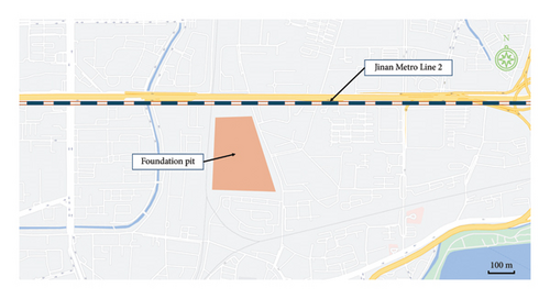
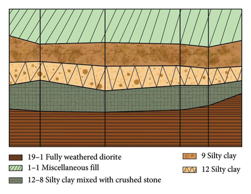
The Jinan Metro Line 2 typically stretches from west to east, with a construction site situated a mere 400 m from the subway’s path, as depicted in Figure 1. The construction site’s strategic placement at this distance is designed to mitigate any negative effects on the current operational tunnels during the excavation of the foundation pit. Continuous, real-time monitoring of the subway tunnel’s deformation at this precise spot is essential for swiftly taking appropriate countermeasures. The geological profile, derived from drilling and presented in Figure 2, reveals that the first 80 m of subsurface strata are predominantly made up of Quaternary Holocene alluvial sediments along with the recent sedimentation. The layers consist of 1-1 miscellaneous fill soil, nine fine-grained clay, 12 fine-grained clay, 12–8 fine-grained clay interspersed with crushed stone, and 19–1 fully weathered plagioclase. It is important to highlight that the subway tunnel functions within the nine fine-grained clay layer.

Details are in the caption following the image — **Figure 1**
Open in figure viewer PowerPoint

The layout of the monitoring zone.

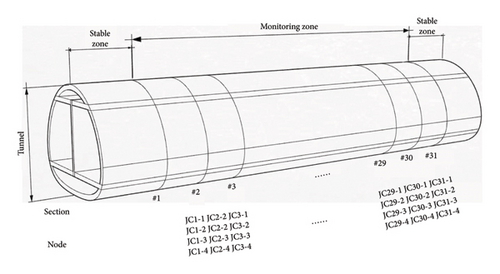
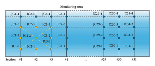
The minimum distance from the tunnel bottom to the arch crown ranges from 5.4 to 10.64 m, with a tunnel inner diameter of 5.8 m. To minimize the impact of tunnel construction on road traffic and ensure subway normalcy, 31 specified monitoring sections were calibrated using a total station method within the monitoring area, uniformly distributed at 10-m intervals. Subsequently, as shown in Figure 3, four monitoring points were allocated on the walls and arch crowns of each section, and real-time data automatic monitoring was conducted using the RTS. The three-dimensional coordinate information of tunnel deformation describes the geometric details of different points on various working faces inside the tunnel. Real-time monitoring coordinate data can be used to continuously analyze tunnel deformation, displacement, and trends, enabling dynamic safety assessments and timely decision-making. With the assistance of RTS and a cloud server system, real-time monitoring data can be automatically collected and transmitted to the cloud server.

3. Methodology

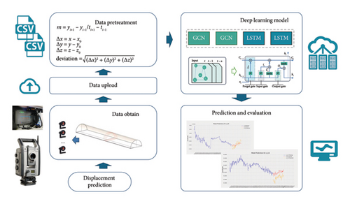
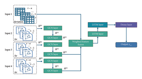
The real-time monitoring and prediction of tunnel deformation are significant for ensuring the safe operation of metro tunnels. In this study, tunnel deformation prediction is based on data acquired from an RTS. This section proposes a hybrid deep learning method combined two neural network models, GCN and LSTM. The process of the method is shown in Figure 4.

3.1. Data Pretreatment

In this research, the goal of forecasting is to predict the displacement in a certain period of time based on the historical displacement information of the metro tunnel. Before the prediction phase, three preprocessing tasks need to be performed.

3.1.1. Data Cleansing

The data cleansing phase includes two steps, outlier handling and missing value imputation.

In this study, multiple group data were collected per day. To ensure a consistent time interval in the training data, each day is treated as a time unit for prediction. Therefore, multiple sets of (x, y, z) coordinate data obtained each day are determined for that day by taking the average. However, due to various factors such as environmental conditions and subway operations, some data clearly exhibit errors and deviate from normal values. Such data, known as outliers, need to be removed before calculating the average. Ensure that the model training is conducted on cleaner and more reliable data, thereby improving the accuracy and robustness of the model.

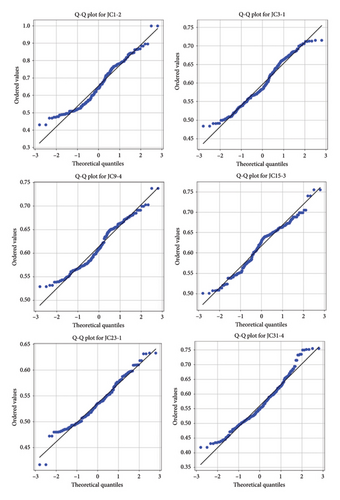
In our study, the Z-score is utilized in outlier detection. One of the primary advantages of the Z-score method lies in its standardization technique, allowing data to be transformed into a standardized normal distribution with consistent scales and units for easy comparison of different variables. Its straightforward and intuitive calculation, coupled with the flexibility to adjust the threshold for outlier detection, makes it easy to implement and fine-tune. Additionally, the interpretability of the Z-score is strong, as it denotes the deviation of data points from the mean, facilitating a clear understanding of the distribution of data [53]. To validate the normality assumption underlying the Z-score method, six random subsamples were extracted from the dataset. The resulting Q-Q plot (Figure 5) demonstrates that the points closely align with the 45° reference line, providing robust evidence that the dataset adheres to a normal distribution. This finding scientifically justifies the application of the Z-score method for subsequent analyses, including outlier detection and standardization procedures.

Assume for Node A and Date B, there are n monitoring data available, shown as a vector x. Then, the mean value of the vector is

()

Then, the standard deviation can be calculated in the following equation.

()

For each data point x_i, subtract the mean μ and divide by the standard deviation σ.

()

Take threshold as 2, corresponding to a 95% confidence level in a normal distribution. The outliers can be detected by the formula below.

()

Then, the average of the valid data can be calculated in the following equation.

()

where y_i represents the i^th valid data point, and m denotes the total number of valid data points.

By aggregating the data, a dataset is generated with a daily time series. The formulas below are used to determine the missed data by linear interpolation.

()

where the date missed value is t_i, corresponding missed value is y_i, and the data of i₋₁ and i₊₁ represent the days before and after the date missed value, respectively.

3.1.2. Statistical Features and Feature Combinations

Statistical features encompass basic data descriptions, such as mean and variance, aiding in summarizing the distribution and central tendencies of the data. Feature combinations, on the other hand, enhance the model’s expressive power by creating new features through the combination of the existing ones. This approach better captures complex relationships and nonlinear patterns, thereby improving model performance and generalization capabilities.

In our study, the gap value between the measurement coordinate data established through statistical features and the original coordinate data better reflects the model’s ability to express the data. The deviation formed through feature combinations can directly represent the deformation characteristics of the tunnel. Hence, for one node, there is a total of seven features for the prediction. The features are x, y, z, Δx, Δy, Δz, and deviation, respectively. The features Δx, Δy, Δz, and deviation can be calculated by the following formulas.

()

where (x₀, y₀, z₀) and (x, y, z) denote to the initial and the obtained position coordinate of the nodes, and the Δx, Δy, and Δz represent the gaps between them. The displacement relies to the prediction of deviation.

3.1.3. Normalization

Data normalization and rescaling are aimed at improving the effectiveness of model training, ensuring that the different scales of features do not lead to instability in model performance. For the specific node and specific feature, the normalization is conducted by the max–min method, as the following formula.

()

where x, x_min, and x_max denote the corresponding x, the minimum, and maximum values of the alternative dataset.

3.2. The GCN-LSTM Model

In this research, a multiple input GCN-LSTM model is proposed for the prediction of deviation, according to the data obtained from the RTS, and is stored in the cloud server, and the data format is comma-separated values (CSV). The initial positions and information of the nodes are also stored as an individual CSV file. Afterward, the real-time monitoring data are uploaded to the cloud server. After the data pretreatment phase, the proposed GCN-LSTM model will be developed to conduct the predictions for the displacement of the tunnel.

As a hybrid model integrated by GCN and LSTM, the proposed method consists of GCN and LSTM cells. The GCN have demonstrated powerful capabilities in addressing graphical correlation problems, the interplay between multiple features has gradually gained attention in tunnel engineering [54, 55], excels in capturing both long-range dependencies and nuanced distinctions between nodes, and has demonstrated notable efficacy in predicting the health status of tunnels [8].

As shown in Figure 6, the model includes four inputs. Input 1 is the deviation of each node. The deviation should be calculated according to equation (10), as is shown in Table 1. Input 2 to Input 4 represent Δx, Δy, and Δz, respectively. The data of the inputs are determined by the RTS, as shown in Figure 7.

Table 1. The deviation input of the prediction model.

Section	Position	Node	Unit	Resource	Symbols
1	2	JC1-2	(mm)	Equation (10)
1	4	JC1-4	(mm)	Equation (10)
1	1	JC1-1	(mm)	Equation (10)
…	…	…	…	…	…
31	2	JC31-2	(mm)	Equation (10)
31	1	JC31-1	(mm)	Equation (10)

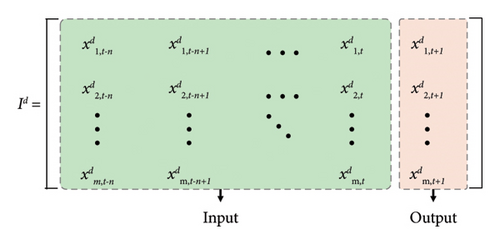
At a given timestamp t + 1, the objective is to predict the values of m nodes using historical monitoring data from the preceding n moments (from t − n to t). Figure 7 shows the input and output of deviation.

To improve the accuracy of the prediction, the GCN is applied to capture the influence of network topology.

The displacement of three dimensions Δx, Δy, and Δz is assigned in Input 2 to Input 4, as shown in Table 2 and equation (10).

Table 2. The Δx, Δy, and Δz inputs of the prediction model.

Section	Position	Node	Unit	Resource	Symbols
1	2	JC1-2	(mm)	RTS
1	4	JC1-4	(mm)	RTS
1	1	JC1-1	(mm)	RTS
…	…	…	…	…	…
31	2	JC31-2	(mm)	RTS
31	1	JC31-1	(mm)	RTS

()

where p represents the three dimensions Δx, Δy, and Δz.

In this work, monitoring node network G is established for GCN cells. An unweighted graph G = (V, E) is utilized to describe the structure of the monitoring zone network, and the monitoring nodes are integrated as follows:

()

where E represents the edge between nodes. We use an adjacency matrix A to illustrate the connection between monitoring nodes; then, we have

()

In tunnel monitoring, the interdependence among monitoring points may correlate with their spatial positions within the tunnel. If the monitoring points are in close proximity, they are likely to be influenced by similar geological conditions, construction impacts, or other external factors, suggesting a potential correlation in their displacement data. By taking into account the precise locations of the monitoring points, the geometric shape of the tunnel, and the actual distances between the monitoring points, if the points are sufficiently close, they can be considered to have a significant mutual influence, denoted by a value of 1 in the adjacency matrix to represent their connection.

As illustrated in Figure 8, taking “JC2-2” as an example, if the surrounding orange nodes are spatially adjacent and, according to the layout of the monitoring points and the specific conditions of the tunnel, these nodes are deemed to influence each other, then in the adjacency matrix, the connections between “JC2-2” and these orange nodes can be represented by 1. For nodes of other colors that are not adjacent to “JC2-2” or have a lesser impact, the corresponding values in the adjacency matrix are set to 0.

Based on the aforementioned definitions, the adjacency matrix A can be established.

For each element Δx, Δy, and Δz, it is essential to establish an integrated network model based on GCN and LSTM. The data reframing process is to be rearranged as a time-series–supervised learning problem. The input of Δx, Δy, and Δz for GCN is

()

Here, is obtained by adding the identity matrix I to the adjacency matrix A of the graph with the formula . is the degree matrix generated from the adjacency matrix A.

At the feature fusion layer, a concatenation method is applied in this model to capture multisource information. Concatenation enhances neural networks by merging diverse features, deepening pattern recognition capabilities. It optimizes deep learning models through feature synergy and streamlined architecture, balancing efficiency with performance.

Afterward, because of the prowess in managing long-term dependencies and their reliability in learning from sequential data, LSTM is used for prediction. LSTM is a powerhouse in the world of neural networks, particularly when it comes to sequence modeling and handling time-series data. It is a kind of the RNN that is designed to keep a long-term memory, overcoming the common issue of vanishing gradients that can trip up standard RNNs, as shown in Figure 9.

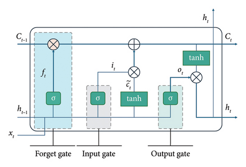
What makes LSTMs tick is their smart structure, featuring a memory cell and three key gates: the input gate, output gate, and forget gate. Think of the memory cell as a conveyor belt that keeps information flowing through the network. The input gate decides what new information to stash in the cell, the forget gate figures out what to toss out, and the output gate calls the shots on what to reveal at each step.

The steps of the LSTM unit are shown in Table 3.

Table 3. The steps of the LSTM unit.

Step	Mathematical expression	Variable
1. Forget gate update	f_t = σ(W_f·[h_t−1, x_t] + b_f)	f_t: The activation of the forget gate at time step t W_f: The weight matrix for the forget gate b_f: The bias term for the forget gate

2. Candidate memory cell		: The candidate memory cell at time step W_c: The weight matrix for the candidate memory cell b_c: The bias term for the candidate memory cell

3. Memory cell update		C_t: The memory cell state at the current time step i_t: The activation of the input gate at the current time step

4. Input gate update	i_t = σ(W_i·[h_t−1, x_t] + b_i)	—

5. Output gate update	o_t = σ(W_o·[h_t−1, x_t] + b_o)	—

6. Final hidden state	h_t = o_t∗tanh(C_t)	—

The deep learning framework that we proposed synergistically merges multiple input streams by harnessing the strengths of both GCN and LSTM networks. This fusion captures the intricate interplay of spatial and temporal dynamics within the input data. Specifically, distinct spatial features are concurrently extracted by the GCN layers, while the sequential LSTM layers are adept at uncovering temporal patterns. The outputs from these distinct yet complementary processes are then strategically concatenated and funneled through a dense layer, resulting in an enriched representation that encapsulates the multifaceted characteristics of the input.

4. Case Study, Result, and Discussion

4.1. Data Description and Pretreatment Phase

The dataset utilized in this study encompasses a comprehensive collection of displacement monitoring data for the Jinan Metro Tunnel, acquired over an extended period to ensure the analysis of tunnel stability and safety. The data were gathered continuously from March 1, 2023, to April 30, 2024, using a high-precision RTS system, which is adept at capturing the minute variations in the tunnel’s structure.

The dataset consists of a substantial volume of records, with each record detailing specific attributes such as node identifiers, initial coordinates, real-time coordinates, and the real-time variation in displacement for each monitoring point in the x, y, and z axes. The total variation in displacement is also documented, providing a cumulative measure of the deformation experienced by each point over the observation period. Despite operational errors, environmental changes, and structural aging affecting some of the 132 monitoring nodes, a total of 106 nodes consistently provided complete data throughout the study duration.

After pretreatment in Section 3.1, Input 1 to Input 4 (deviation, Δx, Δy, and Δz) are well prepared; Table 4 shows the input of deviation.

Table 4. The input description of the deviation.

Input	Count	Min	Max	Mean	Std
	427	0.1837	6.1154	3.4622	1.3429
	427	0.0721	5.3905	3.0184	1.4243
	427	0.1166	5.5454	2.7396	1.1315
	427	1.1105	18.9046	10.1705	7.0871
	427	0.1217	5.0910	2.4639	1.1951
	427	0.4656	7.4678	3.4438	1.3909
	427	0.1929	5.0429	2.5364	1.1155
	427	0.2857	22.4842	7.1591	6.2641
…	…	…	…	…	…
	427	0.1510	9.3013	3.6204	2.0704
	427	0.1414	9.4131	3.2713	2.1340

4.2. The Model Training Phase

The model training process involves the optimization of the deep learning framework that integrates GCN and LSTM networks, as detailed in the previous section. The training is conducted with the aim of minimizing the mean squared error (MSE) loss function, leveraging the Adam optimizer for efficient convergence.

Firstly, multiple datasets at different times are generated using a dynamic window. Then, the LSTM neural network is employed to determine the optimal window size. Finally, the dataset corresponding to the optimal window size is utilized for validation. The training process is meticulously tuned through the careful selection of parameters to ensure robust learning dynamics. The configuration for this training includes a layered approach within the LSTM architecture, with the first layer having 64 neurons and the second layer containing 32 neurons, a design aimed at effectively capturing the intricacies of the data without succumbing to overfitting. The model is subjected to 100 epochs of training, an ample number of iterations that allow for comprehensive learning from the dataset. Additionally, to assess the model’s responsiveness to temporal dynamics, three slide window sizes 5, 10, and 30 are incorporated, representing the number of preceding time steps the model considers for its predictions. The training process is systematically repeated for each look-back period to understand the impact of different historical dependencies on the model’s predictive performance. This parameter setup is intended to provide a nuanced evaluation of the model’s predictive capabilities across varying temporal scopes.

The training procedure begins with data preparation, where the input data are split into training and testing sets, with a ratio of 67% for training and the remainder for testing. For each look-back period specified, the training and testing datasets are further prepared by creating sequences of historical data that the model will use for prediction.

During each epoch, the model’s performance is evaluated on the validation set, and the loss is recorded. The training continues until the specified number of epochs is reached or the performance improvement plateaus.

After the training is completed, the model’s predictions are made on the test set, and the performance metrics, including RMSE, MAE, and WMAPE, are calculated. These metrics provide a comprehensive evaluation of the model’s predictive accuracy.

4.3. The Model Evaluation Phase

After the completion of the model training process, a thorough evaluation is conducted to assess the performance and accuracy of the predictive framework. The evaluation metrics are pivotal in understanding how well the model has learned from the training data and how effectively it can generalize to unseen data.

MSE is a fundamental measure in the assessment of a model’s performance. It represents the average of the squares of the differences between the predicted values and the actual values. Mathematically, MSE is defined as follows:

()

where n is the number of observations, y_i is the actual value of the ith observation, and

is the predicted value for the ith observation. MSE is particularly useful because it penalizes larger errors more than smaller ones due to the squaring operation, which can be beneficial in identifying and mitigating significant prediction errors.

While MSE is a key metric, other metrics provide different perspectives on model accuracy.

RMSE is the square root of MSE and measures the average magnitude of the errors in the same units as the data. It is particularly useful for understanding the scale of the prediction errors and is defined as follows:

()

Unlike MSE, MAE measures the average magnitude of the errors without squaring them, which makes it less sensitive to outliers. It is calculated as follows:

()

WMAPE provides a relative measure of accuracy by weighing the absolute percentage errors by the actual values. It is especially useful when the scale of the predictions varies significantly across different observations.

()

Each of these metrics offers a unique insight into the model’s predictive performance, and they are often used in conjunction to provide a comprehensive evaluation of a model’s effectiveness.

4.4. Result and Discussion

To assess the predictive prowess of our proposed model, this study conducts a comparative analysis with several other models, including the LSTM [56], RNN [57], GRU [58], and ResLSTM [59], and for ease of reference, another GCN-LSTM model with only deviation input which we have designated as GCN-LSTM-2. The comparison of slide window sizes 5, 10, and 30 is shown in Table 5 and Figure 10.

Table 5. Comparison of prediction performances with different deep learning models.

Slide window	5			10			30
Model\metrics	RMSE	MAE	WMAPE	RMSE	MAE	WMAPE	RMSE	MAE	WMAPE
LSTM	0.1359	0.0616	0.1042	0.1376	0.0623	0.1051	0.1499	0.0692	0.1163
RNN	0.1386	0.0681	0.1153	0.1396	0.0684	0.1156	0.1536	0.0808	0.1358
GRU	0.1377	0.0648	0.1097	0.1390	0.0635	0.1071	0.1529	0.0760	0.1278
ResLSTM	0.1366	0.0629	0.1064	0.1398	0.0646	0.1091	0.1495	0.0708	0.1190
GCN-LSTM-2	0.1335	0.0600	0.0932	0.1369	0.0620	0.1045	0.1490	0.0652	0.1102
GCN-LSTM	0.1275	0.0517	0.0917	0.1348	0.0572	0.1011	0.1468	0.0626	0.1098

Note: The bold values represents the proposed method in this paper compared to other methods.

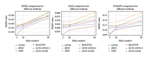
Based on the metrics, we can analyze the performance of the GCN-LSTM model as follows:

Larger sliding windows typically incorporate more historical information; however, the GCN-LSTM model maintains lower error metrics even with smaller windows (such as 5), highlighting its effectiveness in learning from limited data and making precise predictions. Hence, sliding Window 5 is suggested as a better parameter for the dataset.

The GCN-LSTM model consistently demonstrates lower RMSE, MAE, and WMAPE across all considered sliding window sizes (5, 10, and 30), indicating superior predictive accuracy. The model’s performance remains stable across these different window sizes, showcasing its robustness. Notably, for sliding windows 10 and 30, the model achieves even lower RMSE and MAE values compared to other models, underscoring its capability to handle data across varying time scales. When compared to other models such as LSTM, RNN, GRU, and ResLSTM, the GCN-LSTM model consistently achieves lower error metrics, indicating its overall superior predictive performance.

The model’s lower WMAPE values across all sliding window sizes indicate a reduced sensitivity to outliers and the ability to deliver more stable predictions. This stable performance across different time scales enhances the GCN-LSTM model’s practicality for real-world applications, especially in scenarios requiring prompt and accurate forecasting. The GCN-LSTM model exhibits lower errors and higher stability in predictive tasks, distinguishing it from other models. Nonetheless, model selection should account for specific application scenarios and requirements, as well as factors such as model interpretability, training time, and resource consumption.

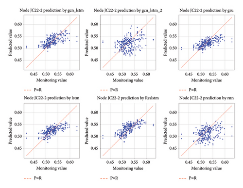
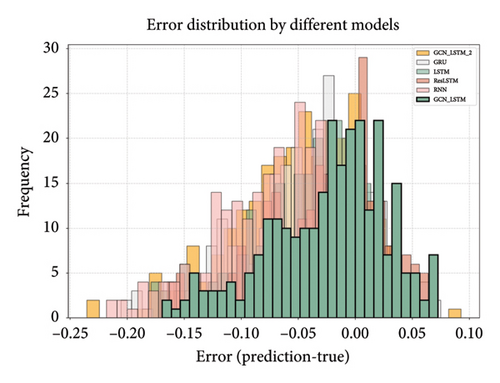
Figures 11 and 12 provide a vivid depiction of the actual and predicted variations at the randomly selected monitoring point JC22-2, illustrating a consistent trend between prediction and observation. The forecasted values align closely with the actual data, showcasing the model’s proficiency in reflecting the deviation changes over time. This visual congruence is further reinforced by the numerical data presented in Table 5 and Figure 10, which quantitatively validates the GCN-LSTM model’s superiority in predictive accuracy compared to other models such as LSTM, RNN, GRU, and ResLSTM. With lower error metrics including RMSE, MAE, and WMAPE, the GCN-LSTM model demonstrates a robust and reliable capability in forecasting displacement values. The collective evidence from both visual and quantitative analysis underscores the GCN-LSTM model’s excellence in predicting metro tunnel displacements, marking it as a preferred choice for such predictive tasks.

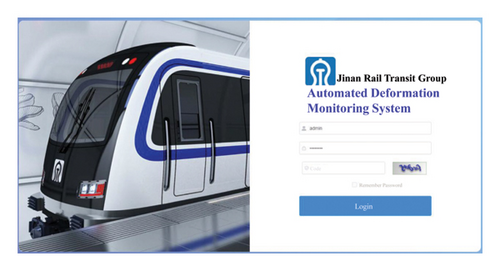
Comprehensive validation through multiple tunnel engineering projects in Jinan further confirms the model’s enhanced robustness under complex geological conditions and varying construction scenarios. The developed monitoring-prediction system has been rigorously validated through multiline engineering applications, with successful implementation across Jinan metro lines (Figure 13). Field deployments under heterogeneous geological and operational conditions demonstrate robust performance, confirming both the methodological generalizability and engineering viability of the proposed framework.

5. Conclusions

This study addresses significant challenges posed by urbanization and construction activities to metro tunnel safety and structural integrity. By introducing a hybrid spatial–temporal deep learning model that integrates GCN and LSTM networks, this research aligns with “dual carbon” goals and enhances the prediction of metro tunnel displacements. The GCN-LSTM model effectively combines GCN’s spatial relationship capture and LSTM’s temporal dynamics handling, providing a robust framework for accurate predictions.

The study developed a real-time monitoring and prediction framework utilizing a RTS for precise data collection, processed and transmitted via cloud servers. This approach not only improves the timeliness of monitoring data but also enhances prediction accuracy. Evaluations against various deep learning models (LSTM, RNN, GRU, and ResLSTM) demonstrate the GCN-LSTM model’s superior performance, validated across different sliding window sizes with lower error metrics and greater stability.

Methodologically, the study includes rigorous data preprocessing steps such as outlier removal, missing value imputation, feature extraction, and normalization. Historical displacement data collected using RTS informs the training of the GCN-LSTM model, evaluated through metrics such as RMSE, MAE, and WMAPE. Case studies, such as the analysis of Jinan Metro Line 2, underscore the model’s reliability for proactive maintenance and sustainable urban development.

Looking ahead, future research will focus on further enhancing the GCN-LSTM model’s accuracy and applicability. This includes integrating environmental factors such as climate and precipitation, refining the model to better reflect real-world displacement patterns, and optimizing neural network architectures. Leveraging multimodal data sources such as geospatial data and construction logs will enrich input features, providing a comprehensive understanding of factors influencing tunnel displacements. Scalability testing across diverse metro systems will ensure broader deployment and support the resilience of urban rail transit infrastructure.

Ethics Statement

This article does not contain any studies with human participants or animals performed by any of the authors.

Conflicts of Interest

The authors declare no conflicts of interest.

Author Contributions

Conceptualization: all authors; methodology: Limin Jia; data collection: Jianfeng Liu; data Analysis: Jianyong Chai; writing – original draft preparation: Jianyong Chai and Zhe Chen.

Funding

This research was supported by the National Key Research and Development Program of China (grant number: 2021YFB2601300) and the National Natural Science Foundation of China (grant number: 71801009).

Acknowledgments

The research was supported by the National Key Research and Development Program of China (2021YFB2601300) and the National Natural Science Foundation of China (71801009).

Open Research

Data Availability Statement

The data that support the findings of this study are available on request from the corresponding author. The data are not publicly available due to privacy or ethical restrictions.

References

1 Miliutenko S., Åkerman J., and Björklund A., Energy Use and Greenhouse Gas Emissions During the Life Cycle Stages of a Road Tunnel-The Swedish Case Norra Länken, European Journal of Transport and Infrastructure Research. (2012) .
Google Scholar
2 Xia Z., Mao J., Chen G., Wu D., and He Y., Decision Criteria and Intelligent Decision Method for Tunnel Excavation Scheme Selection Considering Carbon Emissions, Frontiers of Environmental Science. (2022) 10, https://doi.org/10.3389/fenvs.2022.972677.
10.3389/fenvs.2022.972677
Web of Science® Google Scholar
3 Wang Y., Kou L., He X., Li W., Liang H., and Shi X., A Modified Process Analysis Method and Neural Network Models for Carbon Emissions Assessment in Shield Tunnel Construction, Sustainability. (2023) 15, no. 12, https://doi.org/10.3390/su15129604.
10.3390/su15129604
Web of Science® Google Scholar
4 Bu T., Jiang Z., He M., Hua K., and Wu F., Development of Intelligent Coal Mine Carbon Emission Management System Under Double Carbon Target, Second International Conference on Sustainable Technology and Management (ICSTM 2023). (2023) .
10.1117/12.3007249
Google Scholar
5 Yang L., Wang Y., Han S., and Liu Y., Urban Transport Carbon Dioxide (CO2) Emissions by Commuters in Rapidly Developing Cities: The Comparative Study of Beijing and Xi’an in China, Transportation Research Part D: Transport and Environment. (2019) 68, 65–83, https://doi.org/10.1016/j.trd.2017.04.026, 2-s2.0-85019656423.
10.1016/j.trd.2017.04.026
Web of Science® Google Scholar
6 Li Y., He Q., Luo X., Zhang Y., and Dong L., Calculation of Life-Cycle Greenhouse Gas Emissions of Urban Rail Transit Systems: A Case Study of shanghai metro, Resources, Conservation and Recycling. (2018) 128, 451–457, https://doi.org/10.1016/j.resconrec.2016.03.007, 2-s2.0-84961226628.
10.1016/j.resconrec.2016.03.007
Web of Science® Google Scholar
7 Huang M., Li H., Yu J., Zhang C., and Ni Y., Approach for Evaluating Longitudinal Deformation of Underlying Tunnels Due to Excavation of Upper Foundation Pit (In Chiese), Chinese Journal of Geotechnical Engineering. (2023) 45, no. 11, 2209–2216.
Google Scholar
8 Tan X., Chen W., Yang J., and Tan X., Temporal–Spatial Coupled Model for Multi-Prediction of Tunnel Structure: Using Deep Attention-Based Temporal Convolutional Network, Journal of Civil Structural Health Monitoring. (2022) 12, no. 3, 675–687, https://doi.org/10.1007/s13349-022-00574-4.
10.1007/s13349-022-00574-4
Web of Science® Google Scholar
9 Cha Y.-J., Ali R., Lewis J., and Büyüköztürk O., Deep Learning-Based Structural Health Monitoring, Automation in Construction. (2024) 161, https://doi.org/10.1016/j.autcon.2024.105328.
10.1016/j.autcon.2024.105328
Web of Science® Google Scholar
10 Gómez J., Casas J. R., and Villalba S., Structural Health Monitoring With Distributed Optical Fiber Sensors of Tunnel Lining Affected by Nearby Construction Activity, Automation in Construction. (2020) 117, https://doi.org/10.1016/j.autcon.2020.103261.
10.1016/j.autcon.2020.103261
Web of Science® Google Scholar
11 Liu J. and Zou T., Identifying the Outlier in Tunnel Monitoring Data: An Integration Model, Computer Communications. (2022) 188, 145–155, https://doi.org/10.1016/j.comcom.2022.03.002.
10.1016/j.comcom.2022.03.002
Web of Science® Google Scholar
12 Liu J., Zhang Y., and Wang S., Data Reconstruction for Tunnel Structural Health Monitoring: An Updated KNN Model with Gray Relational Analysis, Marine Georesources & Geotechnology. (2024) 43, no. 4, 646–654, https://doi.org/10.1080/1064119x.2024.2349801.
10.1080/1064119x.2024.2349801
Web of Science® Google Scholar
13 Li H.-N., Ren L., Jia Z.-G., Yi T.-H., and Li D.-S., State-of-the-Art in Structural Health Monitoring of Large and Complex Civil Infrastructures, Journal of Civil Structural Health Monitoring. (2016) 6, no. 1, 3–16, https://doi.org/10.1007/s13349-015-0108-9, 2-s2.0-84959374564.
10.1007/s13349-015-0108-9
PubMed Google Scholar
14 Domaneschi M., Casciati S., Catbas N., Cimellaro G. P., Inaudi D., and Marano G. C., Structural Health Monitoring of In-Service Tunnels, International Journal of Sustainable Materials and Structural Systems. (2020) 4, no. 2/3/4, 268–291, https://doi.org/10.1504/ijsmss.2020.109085.
10.1504/ijsmss.2020.109085
Google Scholar
15 Wang X., Wang M., Jiang R. et al., Structural Deformation Monitoring During Tunnel Construction: a Review, Journal of Civil Structural Health Monitoring. (2024) 14, no. 3, 591–613, https://doi.org/10.1007/s13349-023-00741-1.
10.1007/s13349-023-00741-1
Web of Science® Google Scholar
16 Fahimifar A., Tehrani F. M., Hedayat A., and Vakilzadeh A., Analytical Solution for the Excavation of Circular Tunnels in a Visco-Elastic Burger’s Material Under Hydrostatic Stress Field, Tunnelling and Underground Space Technology. (2010) 25, no. 4, 297–304, https://doi.org/10.1016/j.tust.2010.01.002, 2-s2.0-77952545827.
10.1016/j.tust.2010.01.002
Web of Science® Google Scholar
17 Wu K., Shao Z., Qin S., Zhao N., and Chu Z., An Improved Nonlinear Creep Model for Rock Applied to Tunnel Displacement Prediction, International Journal of Applied Mechanics. (2021) 13, no. 08, https://doi.org/10.1142/s1758825121500940.
10.1142/s1758825121500940
Web of Science® Google Scholar
18 Cheng C. Y., Dasari G. R., Chow Y. K., and Leung C. F., Finite Element Analysis of Tunnel–Soil–Pile Interaction Using Displacement Controlled Model, Tunnelling and Underground Space Technology. (2007) 22, no. 4, 450–466, https://doi.org/10.1016/j.tust.2006.08.002, 2-s2.0-33947149663.
10.1016/j.tust.2006.08.002
Web of Science® Google Scholar
19 Zhang J.-F., Chen J.-J., Wang J.-H., and Zhu Y.-F., Prediction of Tunnel Displacement Induced by Adjacent Excavation in Soft Soil, Tunnelling and Underground Space Technology. (2013) 36, 24–33, https://doi.org/10.1016/j.tust.2013.01.011, 2-s2.0-84874797713.
10.1016/j.tust.2013.01.011
Web of Science® Google Scholar
20 Yang C., Yin Y., Zhang J., Ding P., and Liu J., A Graph Deep Learning Method for Landslide Displacement Prediction Based on Global Navigation Satellite System Positioning, Geoscience Frontiers. (2024) 15, no. 1, https://doi.org/10.1016/j.gsf.2023.101690.
10.1016/j.gsf.2023.101690
Web of Science® Google Scholar
21 Carleo G., Cirac I., Cranmer K. et al., Machine Learning and the Physical Sciences, Reviews of Modern Physics. (2019) 91, no. 4, https://doi.org/10.1103/revmodphys.91.045002.
10.1103/RevModPhys.91.045002
Web of Science® Google Scholar
22 Janiesch C., Zschech P., and Heinrich K., Machine Learning and Deep Learning, Electronic Markets. (2021) 31, no. 3, 685–695, https://doi.org/10.1007/s12525-021-00475-2.
10.1007/s12525-021-00475-2
Web of Science® Google Scholar
23 Mahesh B., Machine Learning Algorithms-A Review, International Journal of Science and Research. (2019) 9, no. 1, 381–386.
Google Scholar
24 Zhang D., Shen Y., Huang Z., and Xie X., Auto Machine Learning-Based Modelling and Prediction of Excavation-Induced Tunnel Displacement, Journal of Rock Mechanics and Geotechnical Engineering. (2022) 14, no. 4, 1100–1114, https://doi.org/10.1016/j.jrmge.2022.03.005.
10.1016/j.jrmge.2022.03.005
Web of Science® Google Scholar
25 Feng X., Jimenez R., Zeng P., and Senent S., Prediction of Time-dependent Tunnel Convergences Using a Bayesian Updating Approach, Tunnelling and Underground Space Technology. (2019) 94, https://doi.org/10.1016/j.tust.2019.103118, 2-s2.0-85072774067.
10.1016/j.tust.2019.103118
Web of Science® Google Scholar
26 Minini J., Zhang Y., Groslambert M., and Commend S., Finite Element-Based Probabilistic Framework Including Bayesian Inference for Predicting Displacements Due to Tunnel Excavation, Computers and Geotechnics. (2023) 162, https://doi.org/10.1016/j.compgeo.2023.105604.
10.1016/j.compgeo.2023.105604
Web of Science® Google Scholar
27 Zhao H., Chen B., Li S., Li Z., and Zhu C., Updating the Models and Uncertainty of Mechanical Parameters for Rock Tunnels Using Bayesian Inference, Geoscience Frontiers. (2021) 12, no. 5, https://doi.org/10.1016/j.gsf.2021.101198.
10.1016/j.gsf.2021.101198
PubMed Web of Science® Google Scholar
28 Li N., Nguyen H., Rostami J., Zhang W., Bui X.-N., and Pradhan B., Predicting Rock Displacement in Underground Mines Using Improved Machine Learning-Based Models, Measurement. (2022) 188, https://doi.org/10.1016/j.measurement.2021.110552.
10.1016/j.measurement.2021.110552
Web of Science® Google Scholar
29 Zheng G., Zhang W., Zhang W., Zhou H., and Yang P., Neural Network and Support Vector Machine Models for the Prediction of the Liquefaction-Induced Uplift Displacement of Tunnels, Underground Space. (2021) 6, no. 2, 126–133, https://doi.org/10.1016/j.undsp.2019.12.002.
10.1016/j.undsp.2019.12.002
Web of Science® Google Scholar
30 Huang Z.-K., Zhang D.-M., and Xie X.-C., A Practical ANN Model for Predicting the Excavation-Induced Tunnel Horizontal Displacement in Soft Soils, Underground Space. (2022) 7, no. 2, 278–293, https://doi.org/10.1016/j.undsp.2021.07.009.
10.1016/j.undsp.2021.07.009
Web of Science® Google Scholar
31 Kong F., Lu D., Ma Y., Li J., and Tian T., Analysis and Intelligent Prediction for Displacement of Stratum and Tunnel Lining by Shield Tunnel Excavation in Complex Geological Conditions: A Case Study, IEEE Transactions on Intelligent Transportation Systems. (2022) 23, no. 11, 22206–22216, https://doi.org/10.1109/tits.2022.3149819.
10.1109/tits.2022.3149819
Web of Science® Google Scholar
32 Zhang L., Shi B., Zhu H., Yu X. B., Han H., and Fan X., PSO-SVM-based Deep Displacement Prediction of Majiagou Landslide Considering the Deformation Hysteresis Effect, Landslides. (2021) 18, no. 1, 179–193, https://doi.org/10.1007/s10346-020-01426-2.
10.1007/s10346-020-01426-2
Web of Science® Google Scholar
33 Pu C., Huang H., and Yang L., An Attention-Driven Convolutional Neural Network-Based Multi-Level Spectral–Spatial Feature Learning for Hyperspectral Image Classification, Expert Systems with Applications. (2021) 185, https://doi.org/10.1016/j.eswa.2021.115663.
10.1016/j.eswa.2021.115663
Web of Science® Google Scholar
34 Liu Z., Wang Y., Li L., Fang X., and Wang J., Realtime Prediction of Hard Rock TBM Advance Rate Using Temporal Convolutional Network (TCN) With Tunnel Construction Big Data, Frontiers of Structural and Civil Engineering. (2022) 16, no. 4, 401–413, https://doi.org/10.1007/s11709-022-0823-3.
10.1007/s11709-022-0823-3
Web of Science® Google Scholar
35 Mahmoodzadeh A., Mohammadi M., Hashim Ibrahim H., Gharrib Noori K. M., Nariman Abdulhamid S., and Farid Hama Ali H., Forecasting Sidewall Displacement of Underground Caverns Using Machine Learning Techniques, Automation in Construction. (2021) 123, https://doi.org/10.1016/j.autcon.2020.103530.
10.1016/j.autcon.2020.103530
Web of Science® Google Scholar
36 Shan F., He X., Armaghani D. J., and Sheng D., Effects of Data Smoothing and Recurrent Neural Network (RNN) Algorithms for Real-Time Forecasting of Tunnel Boring Machine (TBM) Performance, Journal of Rock Mechanics and Geotechnical Engineering. (2024) 16, no. 5, 1538–1551, https://doi.org/10.1016/j.jrmge.2023.06.015.
10.1016/j.jrmge.2023.06.015
Web of Science® Google Scholar
37 Tan X., Chen W., Tan X., Zou T., and Du B., Prediction for the Future Mechanical Behavior of Underwater Shield Tunnel Fusing Deep Learning Algorithm on SHM Data, Tunnelling and Underground Space Technology. (2022) 125, https://doi.org/10.1016/j.tust.2022.104504.
10.1016/j.tust.2022.104504
Web of Science® Google Scholar
38 Chen L., Hashiba K., Liu Z., Lin F., and Mao W., Spatial-Temporal Fusion Network for Maximum Ground Surface Settlement Prediction During Tunnel Excavation, Automation in Construction. (2023) 147, https://doi.org/10.1016/j.autcon.2022.104732.
10.1016/j.autcon.2022.104732
Web of Science® Google Scholar
39 Wu Z., Pan S., Chen F., Long G., Zhang C., and Yu P. S., A Comprehensive Survey on Graph Neural Networks, IEEE Transactions on Neural Networks and Learning Systems. (2021) 32, no. 1, 4–24, https://doi.org/10.1109/tnnls.2020.2978386.
10.1109/TNNLS.2020.2978386
PubMed Web of Science® Google Scholar
40 Zhao L., Song Y., Zhang C. et al., T-GCN: A Temporal Graph Convolutional Network for Traffic Prediction, IEEE Transactions on Intelligent Transportation Systems. (2020) 21, no. 9, 3848–3858, https://doi.org/10.1109/tits.2019.2935152.
10.1109/TITS.2019.2935152
Web of Science® Google Scholar
41 Fu X., Pan Y., and Zhang L., A Causal-Temporal Graphic Convolutional Network (CT-GCN) Approach for TBM Load Prediction in Tunnel Excavation, Expert Systems with Applications. (2024) 238, https://doi.org/10.1016/j.eswa.2023.121977.
10.1016/j.eswa.2023.121977
Web of Science® Google Scholar
42 Ma Z., Mei G., Prezioso E., Zhang Z., and Xu N., A Deep Learning Approach Using Graph Convolutional Networks for Slope Deformation Prediction Based on Time-Series Displacement Data, Neural Computing & Applications. (2021) 33, no. 21, 14441–14457, https://doi.org/10.1007/s00521-021-06084-6.
10.1007/s00521-021-06084-6
Web of Science® Google Scholar
43 Chen J., Wang X., and Xu X., GC-LSTM: Graph Convolution Embedded LSTM for Dynamic Network Link Prediction, Applied Intelligence. (2022) 52, no. 7, 7513–7528, https://doi.org/10.1007/s10489-021-02518-9.
10.1007/s10489-021-02518-9
Web of Science® Google Scholar
44 Fu X., Wu M., Ponnarasu S., and Zhang L., A Hybrid Deep Learning Approach for Dynamic Attitude and Position Prediction in Tunnel Construction Considering Spatio-Temporal Patterns, Expert Systems with Applications. (2023) 212, https://doi.org/10.1016/j.eswa.2022.118721.
10.1016/j.eswa.2022.118721
Web of Science® Google Scholar
45 Ba B., MixHop Graph WaveNet for Traffic Forecasting, Communications in Computer and Information Science, 2022, Springer Nature Singapore, Singapore, 117–131.
Google Scholar
46 Sun A. Y., Jiang P., Mudunuru M. K., and Chen X., Explore Spatio-Temporal Learning of Large Sample Hydrology Using Graph Neural Networks, Water Resources Research. (2021) 57, no. 12, https://doi.org/10.1029/2021wr030394.
10.1029/2021WR030394
Web of Science® Google Scholar
47 Han Y., Hao Y., Feng M. et al., Novel STAttention GraphWaveNet Model for Residential Household Appliance Prediction and Energy Structure Optimization, Energy. (2024) 307, https://doi.org/10.1016/j.energy.2024.132582.
10.1016/j.energy.2024.132582
Web of Science® Google Scholar
48 Zhu J., Wang Q., Tao C., Deng H., Zhao L., and Li H., AST-GCN: Attribute-Augmented Spatiotemporal Graph Convolutional Network for Traffic Forecasting, IEEE Access. (2021) 9, 35973–35983, https://doi.org/10.1109/access.2021.3062114.
10.1109/ACCESS.2021.3062114
Web of Science® Google Scholar
49 Wang X., Liu J., Lin H., Garg S., and Alrashoud M., A Multi-Modal Spatial–Temporal Model for Accurate Motion Forecasting With Visual Fusion, Information Fusion. (2024) 102, https://doi.org/10.1016/j.inffus.2023.102046.
10.1016/j.inffus.2023.102046
Web of Science® Google Scholar
50 Zhang W.-S., Yuan Y., Long M., Yao R.-H., Jia L., and Liu M., Prediction of Surface Settlement Around Subway Foundation Pits Based on Spatiotemporal Characteristics and Deep Learning Models, Computers and Geotechnics. (2024) 168, https://doi.org/10.1016/j.compgeo.2024.106149.
10.1016/j.compgeo.2024.106149
Web of Science® Google Scholar
51 Sun H., Chen Y., Zhang J., and Kuang T., Analytical Investigation of Tunnel Deformation Caused by Circular Foundation Pit Excavation, Computers and Geotechnics. (2019) 106, 193–198, https://doi.org/10.1016/j.compgeo.2018.11.001, 2-s2.0-85056220973.
10.1016/j.compgeo.2018.11.001
Web of Science® Google Scholar
52 Sun H., Wang L., Chen S., Deng H., and Zhang J., A Precise Prediction of Tunnel Deformation Caused by Circular Foundation Pit Excavation, Applied Sciences. (2019) 9, no. 11, https://doi.org/10.3390/app9112275, 2-s2.0-85067226227.
10.3390/app9112275
Google Scholar
53 Smiti A., A Critical Overview of Outlier Detection Methods, Computer Science Review. (2020) 38, https://doi.org/10.1016/j.cosrev.2020.100306.
10.1016/j.cosrev.2020.100306
PubMed Web of Science® Google Scholar
54 Du B., Zou T., Ye J., Tan X., Cheng K., and Chen W., Prediction of Tunnel Mechanical Behaviour Using Multi-Task Deep Learning Under the External Condition, Georisk: Assessment and Management of Risk for Engineered Systems and Geohazards. (2023) 18, no. 1, 275–287, https://doi.org/10.1080/17499518.2023.2182890.
10.1080/17499518.2023.2182890
Web of Science® Google Scholar
55 Li Q., Wang Y., Chen W., Li L., and Hao H., Machine Learning Prediction of BLEVE Loading With Graph Neural Networks, Reliability Engineering & System Safety. (2024) 241, https://doi.org/10.1016/j.ress.2023.109639.
10.1016/j.ress.2023.109639
Web of Science® Google Scholar
56 Zhao Z., Chen W., Wu X., Chen P. C. Y., and Liu J., LSTM Network: a Deep Learning Approach for Short-Term Traffic Forecast, IET Intelligent Transport Systems. (2017) 11, no. 2, 68–75, https://doi.org/10.1049/iet-its.2016.0208, 2-s2.0-85015163282.
10.1049/iet-its.2016.0208
Web of Science® Google Scholar
57 Khandelwal P., Konar J., and Brahma B., Training RNN and It’s Variants Using Sliding Window Technique, 2020 IEEE International Students’ Conference on Electrical,Electronics and Computer Science (SCEECS), 2020, 1–5, https://doi.org/10.1109/sceecs48394.2020.93.
10.1109/sceecs48394.2020.93
Google Scholar
58 Hussain B., Afzal M. K., Ahmad S., and Mostafa A. M., Intelligent Traffic Flow Prediction Using Optimized GRU Model, IEEE Access. (2021) 9, 100736–100746, https://doi.org/10.1109/access.2021.3097141.
10.1109/access.2021.3097141
Web of Science® Google Scholar
59 Tong X., Huang C.-W., Mallidi S. H. et al., Streaming ResLSTM With Causal Mean Aggregation for Device-Directed Utterance Detection, 2021 IEEE Spoken Language Technology Workshop (SLT), 2021, 659–664, https://doi.org/10.1109/slt48900.2021.9383607.
10.1109/slt48900.2021.9383607
Google Scholar

All articles

A Hybrid Spatial–Temporal Deep Learning Method for Metro Tunnel Displacement Prediction Under “Dual Carbon” Background

Abstract

1. Introduction

2. Geological Condition and the Monitoring Points Layout