A Distributed Magnetic Sensor Network: Vehicle Trajectory Tracking Based on Cellular Automaton
Abstract
Magnetic sensor-based vehicle detection is a crucial approach for traffic information collection. However, existing methods that rely on individual magnetic sensors—typically installed at the lane center or roadside—struggle in multilane scenarios due to weak data correlation across sensors and limited accuracy from the isolated sensor. To address these challenges, this paper proposes a novel method that integrates a distributed wireless magnetic sensor network with a temporal-spatial correlation algorithm to associate vehicle signals from multiple sensors. Compared with traditional single-sensor methods, the proposed approach significantly enhances detection reliability by enabling cross-lane vehicle signal fusion. A vehicle position localization technique is introduced to identify detection events, achieving a detection rate of approximately 90%. Experimental results show that while common errors include lane positioning, duplication, omission, and interference, these tend to counteract each other, resulting in a traffic volume detection accuracy of 99.6%. Furthermore, a cellular automaton-based trajectory tracking model is proposed to connect vehicle positions into continuous trajectories, yielding an 89.0% trajectory accuracy and further reducing detection errors. The construction of vehicle trajectories also lays a foundation for future applications such as vehicle speed estimation and vehicle type classification.
1. Introduction
In the field of intelligent transportation systems (ITS), traffic sensing technologies are essential for providing accurate and reliable data to support efficient traffic management. Commonly used detection technologies include inductive loops [1], cameras [2], microwave radar [3], and infrared sensors [4]. Despite their effectiveness, inductive loops face significant limitations due to the need for extensive pavement excavation during installation, which hampers their widespread adoption. Furthermore, the installation and maintenance costs of these systems are relatively high [5]. Cameras, although widely utilized, experience performance degradation in adverse weather conditions such as heavy rain, fog, or when objects obstruct the field of view. Radar and infrared detectors, while effective, are constrained by their high costs. Magnetic sensors present a promising alternative for vehicle detection, offering several advantages including low cost, compact size, low power consumption, and strong resistance to interference under various environmental conditions.
Ferrous metals present in a vehicle’s body disturb the ambient geomagnetic field, enabling vehicle detection via magnetic sensors [6]. Existing studies have primarily focused on sensor deployments either at the roadside [7, 8] or at the center of the lane [9]. Roadside installations are limited to detecting vehicles in the outermost lanes, making them unsuitable for multilane scenarios. Sensors placed at the lane center face challenges in achieving coordinated detection across lanes and are vulnerable to interference from adjacent vehicles. Moreover, current magnetic sensor–based vehicle detection approaches lack effective modeling and association of upstream and downstream vehicle relationships in multilane environments. This issue is exacerbated in complex traffic scenarios such as lane changes, where associating detection results across space and time becomes more difficult. Consequently, it is challenging to infer vehicle dynamics—such as speed and type—based on upstream and downstream sensor data.
- 1.
Design of a magnetic sensor network for spatiotemporal vehicle signal association: A distributed magnetic sensor network is constructed using SRSs, enabling the association of vehicle detection signals across multiple nodes by leveraging both spatial proximity and temporal continuity. This design facilitates robust vehicle recognition in complex multilane environments.
- 2.
Development of a vehicle position localization: A novel localization algorithm is proposed to identify and extract discrete vehicle positions based on magnetic signal patterns. These vehicle positions serve as the foundation for downstream tracking and motion analysis.
- 3.
Trajectory tracking via a CA model: A CA-based method is introduced to model vehicle dynamics and establish logical connections between vehicle positions. This approach enables accurate reconstruction of vehicle trajectories by incorporating lane-specific movement rules and spatiotemporal constraints.
The remainder of this paper is structured as follows: Section 2 reviews prior research on traffic information detection using magnetic sensors, providing the foundation for the proposed approach. Section 3 presents the system architecture of the SRS and outlines the problem formulation. Section 4 describes the method for localizing vehicle positions, while Section 5 explains the vehicle trajectory construction method based on CA. Section 6 evaluates the effectiveness and performance of the proposed methods using data collected from an urban road. Finally, Section 7 concludes the paper, summarizing the key findings and contributions.
2. Related Work
Magnetic sensors have been widely applied in vehicle detection, speed estimation, and vehicle classification [10–12]. Vehicle detection using magnetic sensors typically relies on a single sensor. Feng et al. [5] developed a moving vehicle model to simulate the magnetic field generated by vehicles at different speeds, enabling speed estimation based on detected signals. Wang et al. [13] installed a pair of magnetic sensors in the middle of the lane and applied cross-correlation techniques to estimate vehicle speed. This approach, combined with semiautomated feature extraction, allowed for the determination of vehicle length. Sarcevic et al. [14] employed a three-layer feed forward artificial neural network using time-domain features as inputs for vehicle classification. Tafish et al. [15] utilized discrete Fourier transform and principal component analysis for automatic feature extraction from magnetic signatures and a cost-sensitive support vector machine for vehicle classification. Miklusis et al. [16] proposed an optimal similarity measure function for magnetic sensor signals to facilitate vehicle reidentification, achieving optimal results by linearly combining three signal components (X-Y-Z) [8]. A two-pass moving-average filter is introduced to enhance signal fidelity in low-speed traffic, successfully eliminating high-frequency interference. Similarly, Yang and Lei [17] developed a fixed threshold state machine algorithm based on signal variance to detect vehicles within a single lane in congested, low-speed traffic. Although single-sensor detection simplifies data processing, it faces challenges in handling interference signals, identifying speed, and classifying vehicle types, resulting in limited traffic information acquisition.
Due to the inherent limitations of single-detector systems, multiple sensor approaches have been explored to improve the accuracy of traffic information detection [18, 19]. A common method for vehicle velocity detection involves analyzing the time difference between signals from two magnetic sensors placed along the vehicle’s path [9, 16, 20]. For example, Markevicius et al. [18] used four magnetic sensors to estimate vehicle length based on average speed and signal duration. However, accurate results depend on precise time synchronization between sensors. To address time asynchrony, Feng et al. [7] employed linear discriminant analysis to align measurements from multiple sensors and introduced a magnetometer track-oriented multihypotheses tracker to estimate vehicle trajectories. This method, however, assumes that sensors are roadside-installed and is not suitable for detecting multilane vehicle trajectories.
Multiple cross-sections can detect different positions of the same vehicle simultaneously. By associating these data, vehicle trajectory tracking can be achieved. Trajectory reconstruction is a key research area in traffic studies. Most existing work focuses on fitting and analyzing historical trajectory data to explore traffic flow characteristics and evaluate the safety of transportation infrastructure. For example, Zhao et al. [21, 22] proposed a two-dimensional trajectory reconstruction method based on actual vehicle trajectories and driver behavior factors, which helps analyze traffic flow patterns and supports infrastructure evaluation. However, such approaches mainly rely on historical data mining. In contrast, this study focuses on real-time vehicle trajectory monitoring and reconstruction, offering significant advantages in terms of timeliness.
Trajectory tracking requires the digitization of road space, and CA is a commonly used method for spatial digitization in the field of transportation. CA models have frequently been used to simulate vehicle behavior on roads and analyze traffic states. For instance, Małecki and Wątróbski [23] applied CA to study the effects of traffic rule changes in roundabouts, effectively simulating roundabout sizes and vehicle speeds. Wang et al. [24] extended CA modeling to analyze vehicle-following and lane-changing behaviors in highway ramp segments. The advantage of CA lies in its ability to simulate road geometry and easily formulate vehicle movement rules. In this study, CA is employed to simulate roads and formulate rules for vehicle trajectory tracking.
The key innovation of this research lies in tracking vehicle trajectories using a magnetic sensor network. By integrating signal features from multiple detectors across both time and space, the proposed methods aim to deliver more accurate traffic information.
3. System Architecture and Problem Formulation
In this section, we focus on introducing the proposed detection system and outlining the problem formulation.
3.1. System Architecture
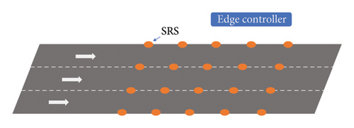
The magnetic sensor network consists of two primary components: the SRSs and the roadside edge controller, as shown in Figure 1. The SRS units are strategically placed on lane markings, and adjacent SRSs across a road section collaborate to detect vehicles passing between them. When a vehicle is detected, the SRS broadcasts packets containing relevant vehicle data to the roadside edge controller via Bluetooth 5.0. The structure of these data packets is detailed in Table 1. To ensure robust communication, each signal message is transmitted 30 times at 300 ms intervals. In the absence of vehicle detection, the SRSs periodically send background magnetic field strength data to the edge controller. The edge controller plays a key role in vehicle tracking by receiving data from approximately 20 SRS units, using this collective information to accurately locate and monitor vehicle trajectories. Moreover, the edge controller serves as a time synchronization hub for the SRSs, which is essential for the fusion of multisensor detection data. Accurate time synchronization is crucial for coordinated detection and precise data integration across multiple sensors.
| Content | Annotation |
|---|---|
| ID | SRS identity number |
| tarrive_time | The starting time of the signal |
| tduring time | The duration of the signal |
| Xmax, Ymax, Zmax, Xmin, Ymin, and Zmin | The maximum and minimum of magnetic field components along the X, Y, and Z axis |
| Xb, Yb, and Zb | The background of the magnetic field along the X, Y, and Z axis |
- 1.
Microcontroller (CC2640): Manufactured by Nordic Semiconductor, it features a Cortex-M4 processor running at a main frequency of 64 MHz and supports Bluetooth low energy communication.
- 2.
Magnetic sensor (RM3100): A PNI magnetic sensor with a measuring range of ±800 μT, operating at a sample frequency of 100 Hz. The orientation of its three axes is predefined relative to the road. The X axis runs perpendicular to the lane, the Y axis is parallel to the X axis and points to the right when aligned with the direction of vehicle travel, and the Z axis is oriented vertically, pointing upwards.
- 3.
Light-emitting diode (LED): Serving as a warning system, the LED alerts drivers to road conditions, making the SRS not only a detector but also an intelligent upgrade to conventional road studs.
- 4.
Rechargeable solar-powered battery: Simplifies the installation process by providing a sustainable power source.
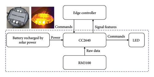
During operation, the RM3100 detects the surrounding magnetic field strength, while the CC2640 processes the raw data to extract vehicle signals. To minimize wireless communication load, only essential signal features are retained and transmitted to the edge controller. This approach ensures efficient data transmission without compromising the accuracy of vehicle detection.
- 1.
Traffic information fusion: The edge controller integrates feature data uploaded by multiple sensors to detect traffic information. This data fusion enhances the accuracy and reliability of the traffic insights obtained.
- 2.
Local traffic control: The edge controller issues local traffic control commands to the SRSs, enabling dynamic management of traffic flow and road conditions.
- 3.
Cloud communication: The edge controller uploads traffic information to the cloud and relays cloud-based commands to the SRSs. The SRSs respond to these commands by adjusting the LED colors, facilitating efficient communication and coordination between the edge controller, the cloud, and the SRSs.
The paper primarily focuses on the first function—traffic information fusion. While a single SRS can provide basic vehicle detection, it struggles in complex situations, such as detecting two vehicles with short headways. To address this, higher-level traffic information detection is necessary. By receiving data from multiple SRSs, the edge controller expands its field of view and achieves significantly higher precision in detecting traffic information.
3.2. Problem Formulation
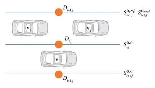
To achieve data fusion, establishing relationships between the signals is essential. Each signal is denoted as , where i and j are the identity number of the signal and represent the index of the SRS that detected the signal. The variable t represents the arrival time of the signal, and v denotes the specific vehicle that induced the signal. In the WSN, signals are correlated in two ways: time correlation and space correlation. These correlations enable the effective combination and analysis of signals from multiple SRSs, resulting in comprehensive and accurate traffic information detection.
TIME correlation: Signals detected by Di,j are linked based on the order of tarrive_time. Multiple signal packets uploaded by different SRSs simulate the sequence of vehicle arrivals. By using time correlation, the system can efficiently identify the most recent signals without searching through all signal packets.
SPACE correlation: Signals induced by the same vehicle and detected by different SRSs in the same column are spatially linked. For example, as shown in Figure 3, the signal detected by Di,j may be induced by more than one vehicle. In such cases, the signal is linked to other signals, such as , on the left, and on the right. Space correlation helps to track the movement of vehicles, facilitating further analysis in subsequent research.
After signal correlation, most detections form multisensor observations, enabling both vehicle position localization and trajectory tracking. As a vehicle passes through the WSN, magnetic sensors at each cross-section capture its signals, which are used to estimate its precise lane-level position—this process is referred to as vehicle position localization. As the vehicle passes multiple cross-sections, a sequence of spatiotemporal vehicle positions is generated. To reconstruct complete trajectories from these discrete positions, we introduce a CA-driven model that associates vehicle positions across sections. Together, they form an integrated framework that significantly improves trajectory reconstruction in multilane, high-density traffic environments, supporting advanced vehicle behavior analysis and traffic management.
4. Vehicle Position Localization
A vehicle position refers to the location of the geometric center of the vehicle. This section focuses on establishing the location of vehicle positions, which will be used for vehicle trajectory tracking.
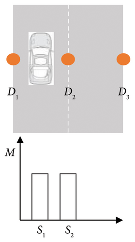
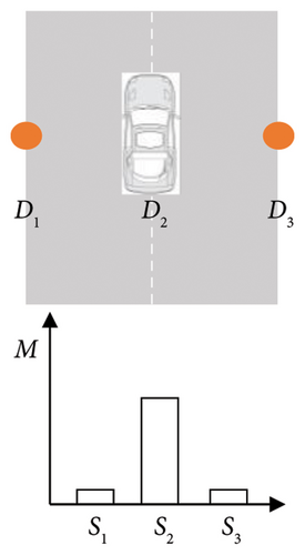
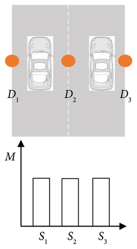
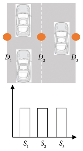
An individual SRS can detect various signals, including interference and signals from multiple vehicles. Previous research [25, 26] has shown that distinguishing between interference signals, single-vehicle signals, and multivehicle signals using a single SRS can be challenging. However, employing multiple SRSs effectively mitigates these issues. To enable comprehensive recognition in complex scenarios, a minimum detection system comprising three SRSs is proposed, as illustrated in Figure 4.
4.1. The Recognition for Interference Signals
4.2. The Recognition for Different Scenarios
- 1.
Single vehicle in the lane (scenario (a) in Figure 4): The magnitude of signals S1 and S2 is sufficient to establish the vehicle’s location. If either S1 or S2 indicates that the vehicle is in the left lane, the vehicle is classified accordingly.
- 2.
Single vehicle on lane markings (scenario (b) in Figure 4): The magnitudes of S1 and S3 are significantly smaller than S2, indicating that they can be classified as interference signals. Therefore, if only an SRS not installed at the roadside detects the vehicle, it is considered to be on the lane markings. Since lane markings are not separately classified in CA models, assigning the vehicle to either the left or right lane is considered valid.
- 3.
Two vehicles (scenario (c) in Figure 4): The magnitudes of S1, S2, and S3 do not show significant differences, allowing for accurate identification of the locations of both vehicles.
- 4.
More than two vehicles (scenario (d) in Figure 4): The left-linked signals of S2 as indicated by space correlation suggest the presence of multiple vehicles. By comparing each signal in the set with S2, the locations of these vehicles can be determined.
Based on the above analysis, Algorithm 1 outlines the method for vehicle position localization. Detailed information regarding each vehicle position is provided in Table 2.
| Attributes | Annotation |
|---|---|
| i, j | The row and column index |
| tarrive time | The arrive time of the vehicle, equal to that of the signal |
| frontVP | The front-connected vehicle position in the trajectory |
| rearVP | The rear-connected vehicle position in the trajectory |
| Signal | The signal that is induced by the vehicle |
-
Algorithm 1: Vehicle position localization.
-
Input: signal S.
-
Output: vehicle position location VP.
- 1.
VP⟵None.
- 2.
ifS is interference signal:
- 3.
VP⟵None
- 4.
else ifS has no left and right linked signals:
- 5.
Establish VP according to S along X axis
- 6.
else ifS has right linked signals:
- 7.
ifS or its right linked signals indicating that the vehicle is in the right lane
- 8.
VP⟵right lane
- 9.
end if
- 10.
end if
-
Remarks: if all the linked signals are interferences, it also indicates that S has no linked signals.
-
VP⟵None indicates no vehicle.
5. Vehicle Trajectory Tracking
This section details the process of tracking vehicle trajectories.
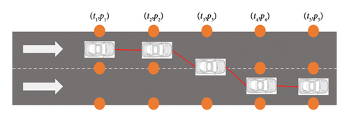
As illustrated in Figure 5, when a vehicle traverses the monitored zone, five vehicle positions are generated, where ti is time stamp and pi is a vehicle position. These vehicle positions collectively form the vehicle’s trajectory. In real-world road scenarios, the WSN must detect multiple vehicles simultaneously.
- 1.
Road simulation: This step simulates the road environment to determine each vehicle’s location.
- 2.
Trajectory construction: The vehicle positions belonging to the same vehicle are connected to form the vehicle’s complete trajectory.
5.1. The Simulation of the Road
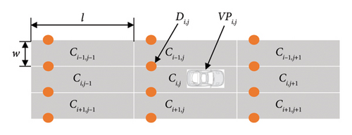
Both vehicle positions and the left-side SRSs of the cells (facing the direction of the vehicle’s movement) share the same row and column index as the cell they are located in. For instance, when a vehicle enters the cell Ci,j, it will be detected by the SRSs: Di,j and Di+1,j. The vehicle position is denoted as VPi,j. This alignment ensures the synchronization of vehicle positions and SRSs with the respective cells, facilitating seamless tracking and correlation of vehicle movement within the CS.
5.2. Trajectory Construction
The essence of trajectory tracking lies in establishing operational rules for vehicles within the CS. These rules are defined as follows:
This indicator F measures the amplitude similarity of two signals, with higher similarity indicating a higher likelihood that the vehicle positions belong to the same vehicle.
- 1.
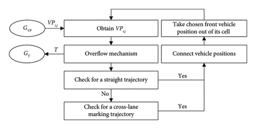
Obtain a Vehicle Position: Take the earliest vehicle position, denoted as VPi,j, from the set of detected vehicle positions, referred to as GVP. Place VPi,j into the corresponding cell Ci,j on the road.
- 2.
Implement the Overflow Mechanism: At the current time tp, examine cells that currently contain vehicle positions. Calculate the duration time td for each vehicle position in its respective cell. If td exceeds the predefined threshold dth, remove the vehicle position from the cell and record its trajectory information T in the trajectory set GT.
- 3.
Check for a Straight Trajectory: If the cell Ci,j−1 is not empty and the head vehicle positions, VPi,j−1, and VPi,j, satisfy the conditions of time continuity, connect the two vehicle positions and remove VPi,j−1 from the cell Ci,j−1. Return to step 1. If there is no vehicle position in Ci,j−1 that meets the TC with VPi,j, proceed to step 4.
- 4.
Check for a Cross-Lane Marking Trajectory: Consider the possibility of two sources of front vehicle positions, from Ci−1,j−1 and Ci+1,j−1. For example, examine Ci−1,j−1. If the head vehicle position VPi−1,j−1 does not meet the conditions for a straight trajectory (i.e., if VPi−1,j−1 and the earliest vehicle position VPi−1,j in GVP from the same lane do not meet the time continuity), then VPi−1,j−1 is considered a part of a cross-lane marking trajectory and can be connected. However, VPi+1,j−1 may also meet the conditions for a cross-lane marking trajectory. In such cases, the indicator F is used to measure the similarity of the signals of the vehicle positions. The trajectory with a higher F value will be chosen as the final connection. The chosen vehicle positions will be removed from its cell. Return to step 1.
- 5.
Extract Remaining Trajectories: Extract all remaining trajectories in the CA and add them to the trajectory set GT.
5.3. Trajectory Error Handling
The entire process of trajectory tracking involves several steps, including signal extraction, interference identification, vehicle position localization, and trajectory construction. Errors can occur at each of these stages, leading to two main types of errors in the final tracked trajectories: incomplete trajectories and repeated trajectories. This subsection discusses the causes of these errors and the methods for correcting them.
- 1.
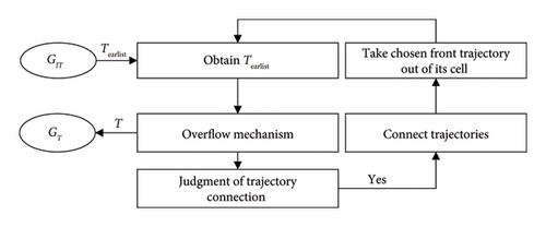
Prepare incomplete trajectories: Extract trajectories from GT with fewer than 5 columns, identifying them as incomplete trajectories. Place these trajectories into the set GIT and sort them by the arrival time tfirst of their first vehicle position in ascending order.
- 2.
Obtain a trajectory: Select the earliest trajectory Tearlist from GIT, and note its first VPfirst and last vehicle positions VPlast. Place Tearlist into the CA based on the location of VPlast, with VPlast marking the starting time in its current cell.
- 3.
Overflow mechanism: Using tfirst as the current time, calculate the duration of each trajectory within its cell. If the duration exceeds a threshold dmean (the mean vehicle passage time for the road section), remove the trajectory from its cell and return it to GT.
- 4.
Evaluate trajectory connection: For the trajectory VPfirst, check previous columns starting from the column index of VPfirst, denoted as cfirst. Assess the time difference tdif between the last vehicle position of a candidate preceding trajectory and the first vehicle position of Tearlist. The connection condition is defined as follows:
() -
where tlow and tup are thresholds based on the column distance and vehicle speed range. If multiple trajectories satisfy the condition, prioritize the trajectory with the longest length and shortest row distance for connection. Extract the front incomplete trajectories from the CA, and repeat step 2 to select the next trajectory for connection.
- 5.
Extract remaining trajectories: Remove all remaining trajectories from the CA, and add them to GT.
Repeated trajectories can occur due to two primary reasons: (1) signal extraction errors, such as large or complex vehicles generating multiple signals, and (2) vehicle position localization errors, where a vehicle is detected by two SRSs and both erroneously record the vehicle’s position, resulting in duplicate vehicle positions and trajectories.
6. Experiment and Result Analysis
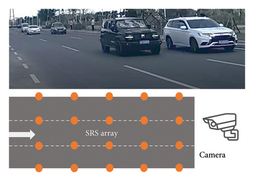
The data used in this study were collected from an urban road in Harbin, China, as shown in Figure 9. The monitored area includes three lanes. To construct the WSN, a grid of 4 rows and 5 columns of SRSs was systematically deployed to capture real-time vehicle data. Simultaneously, a roadside camera was installed to continuously record the entire data collection process. These video recordings were later manually reviewed to obtain accurate ground truth traffic information.
The relevant parameters for vehicle detection and trajectory construction are provided in Table 3.
| Symbol | Description | Value(s) | |
|---|---|---|---|
| fth | A threshold to recognize interference signals | 0.25 | |
| Δtlow | The lower thresholds of time continuity | 0 | |
| Δtup | The upper thresholds of time continuity | 2 | |
| dth | A threshold of duration in the overflow mechanism of trajectory construction | 2 | |
| tlow | The lower threshold of time difference to connect two incomplete trajectories | cd = 1 | 1 |
| cd = 2 | 2 | ||
| cd = 3 | 3 | ||
| tup | The upper threshold of time difference to connect two incomplete trajectories | cd = 1 | 3 |
| cd = 2 | 4 | ||
| cd = 3 | 5 | ||
| dmean | A duration threshold in the overflow mechanism of incomplete trajectory connection | 5 | |
| Δtth | A threshold to judge if two vehicle positions have short arrival time difference | 1 | |
- Note: (1) The data collection process operates on a minimum time scale of 1 s, resulting in all time-related thresholds being rounded to the nearest second. (2) It is important to note that the time-related thresholds utilized in the experiment are specifically tailored for urban roads with vehicle speeds ranging from 30 km/h to 80 km/h. In the context of highway scenes, these thresholds may require adjustment to account for higher vehicle speeds and different traffic conditions.
6.1. Analysis for the Results of the Vehicle Position Location
Table 4 presents the results of vehicle position localization, showing that approximately 90% of the detected vehicle positions are correctly identified. However, four types of error vehicle positions have been observed: lane location error (LLE), repeat error (RE), miss error (ME), and interference error (IE). These errors can be attributed to the following factors:
| Column | 1 | 2 | 3 | 4 | 5 | |
|---|---|---|---|---|---|---|
| Correct | Number Q | 508 | 501 | 506 | 507 | 505 |
| Proportion | 92.2% | 91.9% | 89.7% | 93.9% | 89.7% | |
| LLE | 14 | 18 | 13 | 10 | 11 | |
| RE | 26 | 25 | 39 | 21 | 40 | |
| ME | 29 | 33 | 31 | 34 | 33 | |
| IE | 3 | 1 | 6 | 2 | 7 | |
| Number of vehicle positions | Total detected traffic volume | 551 | 545 | 564 | 540 | 563 |
| Mean detected traffic volume Qmean | 553 | |||||
| Real traffic volume QReal | 551 | |||||
| Accuracy | 99.6% | |||||
- Note: Proportion = Q/QReal and Accuracy = 1-|Qmean − QReal|/QReal.
LLE: The disturbance direction of the signal along the X axis is generally effective in determining the vehicle location, but a small number of errors can occur. Previous research [25] has shown that such errors are more likely when the magnetic field component in the vertical direction from a vehicle is weak. However, since most areas have a vertical component of Earth’s magnetic field, the occurrence of these errors is quite rare.
RE: REs are primarily caused by large vehicles, vehicles with complex signals, or LLE. This type of error represents a significant portion of all errors and is difficult to eliminate using only individual vehicle positions. However, trajectories constructed from repeated vehicle positions are considered repeated trajectories and are removed during the later stages of processing.
ME: MEs account for a considerable proportion of total errors and arise from two main causes. First, vehicles with low signal amplitudes may be obscured by larger vehicles, causing their signals to be mistaken for interference, leading to a missed detection. Second, when the time headway between vehicles is very short, signals from both the front and rear vehicles may be extracted as a single signal. However, as time headways vary, some SRSs can detect both vehicles. Constructing trajectories helps mitigate MEs through mutual correction.
IE: IEs make up a small percentage of all errors and are typically caused by background noise or system disturbances. Not all columns of SRSs experience these errors, and constructing trajectories allows for mutual correction to address these issues.
Despite approximately 10% of vehicle positions being error-prone, it is noteworthy that the number of missed vehicle positions is nearly balanced by the combined number of repeated and interference signals. This balance results in the total number of detected vehicle positions being close to the actual count. During the detection period, the recorded traffic volume was 551 vehicles, and the average number of vehicle positions detected by different columns of SRSs was 553. This leads to a detection accuracy of 99.6%, demonstrating the system’s reliability.
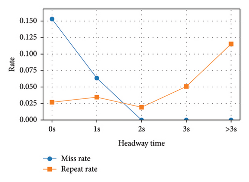
Figure 10 illustrates the distribution of missed detection and duplicate detection rates under varying time headways. When the time headway is short, the incidence of missed detections increases, primarily due to mutual occlusion between vehicles. This effect is particularly pronounced when large and small vehicles travel side by side, as the magnetic signal of the smaller vehicle may be masked, resulting in detection failure. As the time headway increases, the issue of missed detections is significantly alleviated. In contrast, duplicate detections predominantly occur under long time headway conditions, suggesting that the cause is not interference between vehicle magnetic fields, but rather misjudgment triggered by a single vehicle. Case studies reveal that such errors are mainly caused by large vehicles passing independently. As these vehicles traverse the system, they are detected simultaneously by multiple sensors on the same cross-section, leading to a false identification of vehicles in multiple lanes.
6.2. Analysis for the Results of Vehicle Trajectory
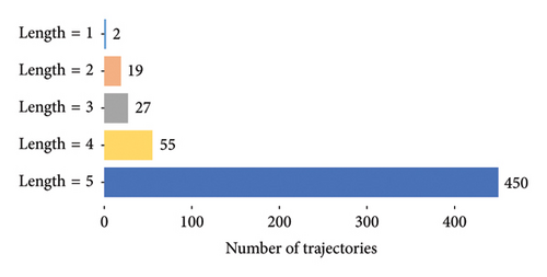
As shown in Figure 11, the distribution of trajectory lengths reveals that, due to missed vehicle positions and the implementation of the overflow mechanism, not all extracted trajectories contain the full set of five vehicle positions. Among the extracted trajectories, 450 trajectories consist of five vehicle positions, accounting for approximately 81.4% of the total. These incomplete trajectories illustrate the process of mutual correction across different columns of SRSs. While a vehicle may be missed by some columns, the likelihood of it being missed by all columns is extremely low. This mutual correction mechanism significantly enhances the overall accuracy of the trajectory tracking process.
As illustrated in Table 5, the term “Correct” refers to trajectories where all vehicle positions belong to the same vehicle, indicating accurate tracking. In contrast, the abbreviations E1, E2, and E3 represent cases where there are 1, 2, and 3 vehicle positions, respectively, in the trajectory that does not belong to the target vehicle (the one with the highest proportion of vehicle positions in the trajectory). “RE” stands for repeated trajectories, which occur when redundant vehicle positions result in duplicate tracking. “NE” indicates interference trajectories caused by background disturbances or system issues. Lastly, “ME” signifies missed vehicles, which result from low signal amplitude or short time headways during detection.
| Type | Correct | E1 | E2 | E3 | RE | IE | ME |
|---|---|---|---|---|---|---|---|
| Number | 492 | 22 | 20 | 2 | 15 | 2 | 15 |
| Total number of trajectories Qtrajectory | 553 | ||||||
| Real traffic volume QReal | 551 | ||||||
| Accuracy | 99.6% | ||||||
| Proportion | 89.0% | 4.0% | 3.6% | 0.04% | 2.7% | 0.04% | |
- Note: Accuracy = 1 − |Qtrajectory − QReal|/QReal and Proportion = Number/Total.
The majority of the trajectories are of the “Correct” type, demonstrating the effectiveness of the proposed method for constructing trajectories. However, the E1, E2, and E3 errors collectively account for approximately 8% of the total trajectories, primarily due to LLEs. Figure 12 illustrates an example of this type of error: vehicle A is correctly detected in Lane 2 at time tA, whereas vehicle B is mistakenly detected in Lane 1 at time tB. If the time difference tB − tA falls within the threshold for temporal continuity, a connection error may occur. To reduce these errors, appropriate lower (0.4 s) and upper (1.8 s) thresholds in time continuity can be applied. However, in our experiment, the time precision is limited to whole seconds, which is insufficient for obtaining highly accurate trajectories. Future research will focus on utilizing smaller time scales to reduce these errors.
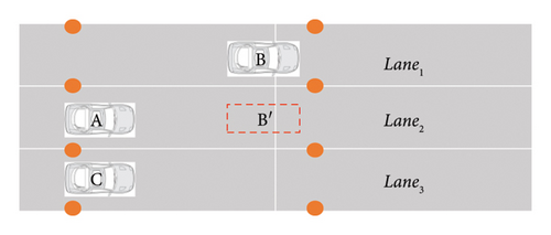
The number of repeated, interference, and missed errors has significantly decreased due to mutual correction achieved through trajectory construction. However, it is important to note that the process of removing repeated trajectories may lead to the omission of some vehicles. For example, in high-density traffic, vehicles such as A and C passing through the monitored area in parallel may result in one of their trajectories being mistakenly identified as a repeated trajectory and subsequently removed. Such occurrences are more frequent in high-traffic scenarios. Additionally, in dense traffic, signals from vehicles with strong magnetic fields may overlap with those from vehicles with weaker magnetic fields, which is a limitation of magnetic sensors.
The predicted traffic volume of 553 demonstrates an accuracy of approximately 99.6%, which is higher than the results detected by most columns of SRSs. While the accuracy matches the average of those results, the predicted volume is considered more reliable due to the reduced occurrence of repeated, interference, and missed errors. Compared to other similar studies on vehicle detection using magnetic sensors, as shown in Table 6, our methods demonstrate higher accuracy and are better suited for multilane scenarios, as shown in the table.
7. Conclusion
The proposed method of tracking vehicle trajectories using multiple distributed magnetic sensors has yielded promising results, with approximately 89.0% of trajectories being accurately extracted. Although some incorrect trajectories were observed, the overall accuracy of detected traffic volume reached 99.6%. Due to the limitations of the time scale in the current study, additional traffic information such as speed and traffic density could not be extracted. Nevertheless, methods for extracting these types of traffic data have been briefly introduced.
- 1.
Future research will focus on improving the time scale of sampled data, and three key directions will be pursued:
- 2.
Evaluating methods to extract traffic information such as speed and density: Future research will aim to develop robust methods to accurately measure vehicle speed and estimate traffic density based on the collected data.
- 3.
Adapting time-related thresholds to vehicle speed: The current study employed fixed time-related thresholds, which may not be optimal for varying vehicle speeds. Future studies will explore adaptive thresholds that adjust based on vehicle speed.
- 4.
Investigating methods for distinguishing vehicle types: Vehicle types are often linked to vehicle length, and accurate speed data are essential for reliable length estimation. Future work will focus on innovative approaches to identify and classify different vehicle types based on their trajectory and speed characteristics.
Conflicts of Interest
The authors declare no conflicts of interest.
Author Contributions
Xinpeng Yao: conceptualization and methodology; Yanli Sun: writing; Mengfei Liu: data analysis; Hua Wang: supervision, funding acquisition, and reviewing; Zijian Wang: reviewing; Wei Quan: reviewing; Wen Rong: reviewing.
Funding
The research work is supported by the State Key Lab of Intelligent Transportation System (Traffic holographic perception network structure and system under linear road features) and the National Natural Science Foundation of China 42171451.
Acknowledgments
The research work is supported by the State Key Lab of Intelligent Transportation System (traffic holographic perception network structure and system under linear road features) and the National Natural Science Foundation of China 42171451.
Open Research
Data Availability Statement
The datasets generated during and/or analyzed during the current study are available from the corresponding author on reasonable request.


