A Study on Fitting Longitudinal Profiles of Railway Station Tracks
Abstract
The accurate fitting of railway station track profiles is crucial for improving the quality of station-related engineering projects. However, in practice, there are still cases where straight lines are used to approximate vertical curve segments. To avoid the ‘straight-line approximation’ deviation in the gradient value of the profile’s straight segments, this paper establishes a mathematical programming model with the objective of minimising the total amount of track raising and lowering. To satisfy the model constraints, an optimal vertical curve fitting algorithm, utilising a bisector vector approach to unambiguously resolve the conjugacy issue in analytical circular curve calculations, and a genetic algorithm based on neighbourhood search, specifically designed to fine-tune initial least squares gradient estimates and avoid systematic deviations, are proposed. Finally, the effectiveness of the proposed model and algorithm is validated through a case study. With a total grade value adjustment of only 0.45‰ based on the least squares method, the proposed fitting algorithm achieves a 38.7% reduction in track raising and lowering compared to manual fitting. This demonstrates the effectiveness of the proposed method in achieving the integrated optimisation of straight-line segments and vertical curve segments within the longitudinal profile. The implementation of this algorithm through programming can significantly enhance both the efficiency and quality of railway station track profile fitting.
1. Introduction
Railway station track alignment design plays a crucial role in ensuring smooth train operation, passenger comfort and efficient freight transport. The longitudinal profile, a critical component of track alignment, dictates the vertical geometry of the track. This geometry directly impacts train acceleration and deceleration characteristics, energy consumption and overall operational efficiency [1]. In the context of railway stations, the accurate representation and optimisation of the longitudinal profile are paramount for various renovation and upgrading projects. These projects might involve track realignment, platform construction, or even the integration of new high-speed rail lines [2]. Precisely capturing the profile ensures the feasibility and accuracy of subsequent design modifications.
However, the longitudinal profiles of railway stations, particularly those constructed in earlier periods, often exhibit irregularities and deviations from ideal geometric curves [3]. This can be attributed to factors like ground settlement over time, track maintenance practices and the limitations of surveying techniques employed during the original construction. Traditional methods of manually fitting straight lines and circular curves to represent the profile can result in inaccuracies, especially in sections with significant vertical transitions [4]. These inaccuracies can lead to problems during construction and operation, including excessive track raising or lowering, abrupt changes in gradient and compromised ride quality.
To address these challenges, this paper proposes a novel approach for fitting the longitudinal profile of railway station tracks. This approach aims to minimise the amount of track raising and lowering required, thereby reducing construction costs and minimising disruptions to existing infrastructure. Specifically, the novelty lies in two key algorithmic contributions integrated within an optimisation framework: (1) an optimal vertical curve fitting algorithm employing a bisector vector method to robustly handle the inherent conjugacy issues in analytical curve calculations, ensuring accurate and unambiguous curve geometry, and (2) a neighbourhood search genetic algorithm (NSGA) strategy designed not for general alignment optimisation from scratch but to intelligently fine-tune initial gradient estimates derived from least squares fitting. This combination is particularly advantageous for reconstructing existing profiles, as it leverages initial data whilst performing a global search to minimise costly track adjustments and simultaneously satisfy complex geometric and operational constraints, offering a more practical and efficient solution compared to standard fitting or general optimisation techniques.
2. Literature Review
Extensive research has been conducted on railway track alignment design and optimisation, with a particular focus on new railway lines. However, the unique challenges associated with fitting railway station track profiles have received relatively less attention. This section reviews the relevant literature in three key areas: (1) traditional railway track alignment design methods, (2) optimisation techniques applied to railway alignment and (3) existing methods for fitting railway track profiles.
2.1. Traditional Railway Track Alignment Design Methods
Traditional railway track alignment design primarily relies on manual methods based on engineering experience and design codes [5]. These methods involve dividing the alignment into straight lines, circular curves and transition curves (typically cubic parabolas) to connect straight segments with circular curves smoothly [6]. Engineers typically rely on their expertise and judgment to determine the appropriate parameters for these geometric elements, ensuring compliance with design standards for grade, curvature and superelevation [7]. Whilst these methods have been successfully applied in numerous railway projects, they can be time-consuming and require significant manual adjustments, especially for complex terrain and railway stations with irregular profiles.
2.2. Optimisation Techniques in Railway Alignment Design
With the advancement of computing power and optimisation algorithms, researchers have explored various optimisation techniques to automate and improve the railway track alignment design process. These techniques aim to find the optimal alignment that minimises construction costs, environmental impacts and/or operational expenses whilst satisfying design constraints [8].
-
Genetic Algorithms (GAs): Inspired by natural selection, GAs have been widely used for railway alignment optimisation due to their ability to handle complex, nonlinear problems with multiple objectives [9–11].
-
Simulated Annealing (SA): SA is a metaheuristic optimisation technique that simulates the annealing process in metallurgy to find the global optimum by gradually decreasing the probability of accepting worse solutions [12].
-
Particle Swarm Optimisation (PSO): Inspired by the social behaviour of bird flocking or fish schooling, PSO iteratively improves candidate solutions based on their position and velocity in the search space [13].
-
Ant Colony Optimisation (ACO): ACO mimics the foraging behaviour of ants to find the shortest path between a food source and the colony, making it suitable for solving routing problems, including railway alignment optimisation [14].
Furthermore, whilst several studies have proposed innovative methods for spatiotemporal data modelling and traffic flow prediction, their direct applicability to railway track profile reconstruction is limited. Monte Carlo tree search (MCTS) [15], whilst effective for path discovery, may struggle with the continuous and constrained nature of track alignment optimisation. Temporal graph convolutional networks (TGCNs) [16] and spatial-temporal dependence models [17], primarily designed for traffic flow prediction, do not readily accommodate the specific geometric constraints and the objective of minimising track raise and lower, which are crucial in track profile reconstruction. Our proposed method addresses these limitations by directly incorporating engineering constraints within a mathematical programming model and employing a GA tailored to this specific application.
2.3. Fitting Railway Track Profiles
Whilst the aforementioned optimisation techniques have shown promise in optimising new railway alignments, their application to fitting railway station track profiles remains limited. The main challenge lies in accurately capturing the track geometry, which often exhibits irregularities and deviations from ideal geometric elements.
-
Least Squares Method: This widely used method minimises the sum of squared errors between measured data points and the fitted curve [18]. However, it can be sensitive to outliers and may not accurately represent the actual track geometry, especially in sections with abrupt changes in gradient.
-
Spline Interpolation: Spline functions, particularly cubic splines, offer a flexible approach for fitting smooth curves to scattered data points [19]. However, selecting appropriate spline parameters and ensuring continuity at knot points can be challenging.
These methods often focus on accurately representing the profile without explicitly considering the minimisation of track raising and lowering during subsequent design modifications.
In summary, whilst existing research provides valuable insights into railway alignment design and optimisation, there is a need for a dedicated approach that addresses the unique challenges of fitting railway station track profiles whilst minimising track raising and lowering. This paper aims to bridge this gap by proposing a novel optimisation model and algorithm specifically designed for this purpose.
3. Problem Description
The key to fitting the longitudinal profiles of railway station tracks lies in determining the locations of points of vertical intersection (PVI). Methods for identifying these points include analysing gradient changes between survey points and consulting technical logbooks maintained by railway maintenance departments [20, 21]. Whilst the precise identification and accuracy of PVI locations are crucial in practical engineering and can influence the final alignment quality, this study presupposes that the PVI mileages are known with sufficient accuracy, typically derived from standard surveying practices and existing railway records. This assumption is made to focus the scope of this paper on the development and validation of the optimal fitting algorithm between these predefined points. Furthermore, the model takes into full account constraints representing essential geometric and operational requirements commonly mandated by railway design standards for station areas, such as the maximum gradient, acceptable levels of track raising and lowering, standard vertical curve radii limits and ensuring vertical curves do not overlap with turnout mileages. These constraints (detailed in equations (2)–(5)) are considered fundamental for ensuring safe and efficient train operations within station limits. Based on these assumptions and constraints, this study aims to derive a fitting solution that satisfies these essential criteria whilst minimising deviation. This problem can be formulated mathematically using the following optimisation model.
-
i: Survey point number (i = 1, 2, ⋯, m);
-
j: PVI number (j = 1, 2, ⋯, n, n + 1), totalling n PVIs. For convenience of expression, the last survey point is designated as PVI n + 1, thereby assigning each number to a corresponding gradient segment.
-
p: Turnout number (p = 1, 2, ⋯, o);
-
: For survey point i, these represent the mileage, actual elevation, fitted elevation and amount of raising or lowering (where , respectively)
-
kj, Rj: The gradient value of segment j and the radius of the vertical curve at PVI j, respectively
-
: The positions of the straight-to-curve and curve-to-straight points when a vertical curve is applied at PVI j; the pair denotes the extent of the vertical curve
-
: Upper and lower limits, respectively, for the amount of raising or lowering Δyi
-
: Upper and lower limits for the radius of the vertical curve
-
: The start and end mileages of turnout p; the pair denotes the extent of turnout p
-
kλ: The threshold limit for the gradient difference between adjacent segments when they are connected by a vertical curve
-
: The maximum gradient allowed for station tracks
Equation (1) represents the objective function, aiming to minimise the total deviation in raising and lowering amounts for the longitudinal profile fitting. Equation (2) constitutes a constraint, stipulating that the fitted gradient values for each segment must not exceed the predefined maximum gradient. Equation (3) is another constraint, accounting for the allowable range of raising and lowering at each survey point after considering factors such as the ballast thickness and overhead contact line height. Equation (4) serves as a constraint, dictating that when the gradient difference between adjacent segments at any PVI exceeds the specified tolerance, a vertical curve must be employed for connection, with its radius kept within predefined limits. Lastly, equation (5) acts as a constraint, ensuring that the range of any vertical curve, necessitated by a gradient difference exceeding the standard at a PVI, does not overlap with the extent of any turnout.
The mathematical model formulated above presents a complex constrained optimisation problem. The objective function, aimed at minimising the total amount of track raising and lowering (equation (1)), can exhibit nonlinear characteristics due to the absolute value function and the conditional inclusion of vertical curves based on gradient differences. Furthermore, the problem involves multiple continuous variables (gradient values for each segment) and a series of practical engineering constraints (equations (2)–(5)), including limitations on maximum gradient, allowable track adjustments, vertical curve parameters and noninterference with turnouts. Traditional deterministic optimisation methods may face challenges in efficiently finding a global optimum for such a problem, particularly given the potential for numerous local optima and the discrete nature of some decisions (e.g., whether to insert a vertical curve). This complexity necessitates an approach capable of exploring a broad solution space whilst effectively managing these diverse constraints.
4. Solutions
This paper assumes that the mileage positions of PVIs are known, implying that the lengths of the gradient segments comply with established standards. The primary focus is on discussing an integrated fitting method for both the straight-line segments and vertical curve segments of the longitudinal profile. The algorithm adopts a fundamental approach of ‘straight-first, then curve, unified fitting’, which entails initially handling straight segments before proceeding to the fitting of vertical curves in a cohesive manner.
- 1.
Based on the identified PVI locations, we employ the least squares method to individually fit the gradient values for each straight-line segment.
- 2.
We sequentially inspect the gradient differences between segments before and after each PVI. If the difference exceeds the limit, incorporate a vertical curve with an appropriate radius for connection.
- 3.
We assess whether the constraints outlined in equation (2) through equation (5) are satisfied. If they are, we iteratively compute whether the deviation in raising and lowering for the fitted profile decreases further. Upon reaching the termination criterion, we output the results; otherwise, we make minor adjustments to the gradient values based on the least squares fitting and continue iterating to optimise the profile.
-
Algorithm 1: Once the gradient values for each segment are determined, during the assessment of the constraints in equations (4) and (5), the fitting of a vertical curve is necessary. The analytical method for computing the circle equation during this fitting process can generate conjugate issues. To address this, a vertical curve fitting technique based on the bisector vector is devised to attain the optimal line shape.
-
Algorithm 2: To mitigate systemic biases that may arise from solely using the least squares method to fit the gradients of straight-line segments in station tracks, a neighbourhood search-based GA is proposed. This algorithm efficiently solves for the best gradient values that satisfy the constraints in equations (1) and (2), ensuring a more accurate fitting under given conditions.
4.1. Optimal Vertical Curve Fitting Algorithm
4.1.1. Conjugacy Issues in Vertical Curve Fitting
The fitting of straight-line segments within railway station tracks essentially involves solving for the optimal gradient of a line passing through a fixed point (with the starting point predefined). The use of vertical curves to connect station track gradient segments is primarily to ensure that when trains pass through PVIs with substantial differences, they do not derail or uncouple, maintain smooth operation, adhere to clearance limits and promote safety. The vertical curve’s geometric characteristic manifests in the tangency of the vertical curve to the two adjacent straight-line segments, as illustrated in Figure 1(a).
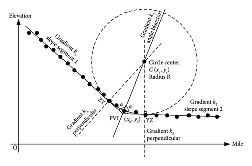
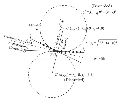
Given the assumptions, after fitting to obtain the linear equations l1 and l2 for the straight-line segments adjacent to the PVI, the bisector line passing through the PVI (x0, y0) must be calculated, as depicted in Figure 1(b). The solution yields two mutually perpendicular bisectors, l3 and , with gradient values , representing a pair of conjugate roots, where A = (k1k2 − 1/k1 + k2). Obviously, if the angle between the PVIs forms an obtuse angle, the selection of the ± sign for k3 should be made by discarding the gradient of the acute angle bisector according to the actual line shape.
After determining the angle bisector line l3, it is necessary to further identify the coordinates of the centre of the circle with radius R. As shown in Figure 1(b), there are two circles that are tangent to both lines l1 and l2. Solving for their centres yields the conjugate centres C′ and C″, with coordinates (xc, yc) = (x0 ± B, y0 ± k3B), where . Clearly, the selection of the ± sign for the vertical curve’s centre should be determined by whether the geometric figure formed by the curve centre, grade change point and its two adjacent measured points constitutes a convex curve. If it does not form a convex curve, the solution should be discarded.
Once the centre of the circle is established, according to the equation of the circle, in solving for the elevation equations that fit the vertical curve segment, we have , which also exhibits conjugacy. Obviously, the choice of the ± sign in this equation can be determined based on the concavity or convexity of the vertical curve.
All three instances of determining the ± signs mentioned above can be resolved by manually predetermining the geometric characteristics of the vertical curve [22].
4.1.2. Method for Vertical Curve Fitting Based on Bisector Vector
To address the issue in Section 4.1.1 where multiple determinations of the ± symbols are required when calculating the fitting equations for vertical curves, and to facilitate computer programming, this paper proposes a fitting method centred around the bisector vector, taking into account the characteristics of railway station track longitudinal profiles. By utilising vector operations to determine the ± symbols during computation, this method eliminates the impact of conjugacy in the fitting process, optimising the calculation procedure and reducing the complexity of finding solutions.
Technically, operation stations’ various yard tracks, external running lines for workshops and sections and internal tracks within workshops and sections are ideally situated on level ground. Different types of lines have distinct maximum gradient limits. For example, the maximum gradient for a high-speed rail maintenance depot’s running line is set at 30‰ (with a challenging value of 35‰). Where algebraic differences exceed these limits and the absolute values of gradients in adjacent segments differ, concave and convex vertical curves can form, manifesting in four distinct configurations, as illustrated in Figure 2. Furthermore, when the sum of the gradient values equals zero, the bisector of the angle is aligned parallel to the vertical axis.
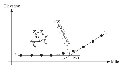
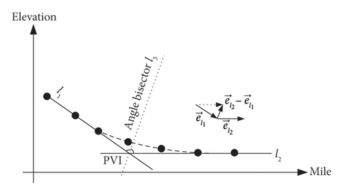
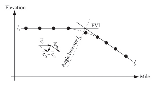
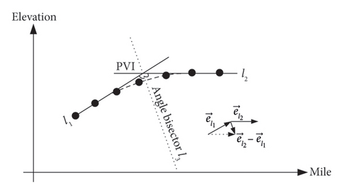
Taking the concave vertical curve type 1 illustrated in Figure 2(a) as an example, during fieldwork involving horizontal measurements moving in a certain direction (for instance, with increasing mileage), the straight lines l1 and l2 represent the segments adjacent to the PVI. Assuming that the gradient values fitted for these straight-line segments using the method described in Section 4.1.1 are k1 and k2, we can then define unit vectors parallel to lines l1 and l2 as and , respectively. Constructing vector in accordance with the subtraction rule for vectors means that vector represents the bisector vector. When a ≠ 0, the gradient of the bisector line can be derived as k3 = (b/a).
To solve for the coordinates of the circle’s centre, after obtaining the conjugate centre coordinates C′ and C″ using the method in Section 4.1.1, one can assess whether the vector formed from this point to the PVI is collinear with the bisector vector , and if they are pointing in the same direction, this identifies the desired centre coordinate.
In determining the appropriate ± sign for the elevation fitting formula, the elevation component b of the vector can serve as the criterion. Evidently, for the bisector in Figures 2(a), 2(b), with the positive ordinate component b > 0, the applicable circle equation is ; conversely, for the bisector in Figures 2(c), 2(d), with the negative ordinate component b < 0, the suitable circle equation becomes .
4.1.3. Algorithm for Optimal Vertical Curve Fitting
Current design specifications stipulate the range of vertical curve radii for railway longitudinal profiles according to different grades or categories, such as a minimum of 600 m for elevated unloading lines and a maximum of 30,000 m for high-speed mainlines. Hence, within these prescribed limits, a traversal scope and a search step size λ can be set according to practical circumstances. Utilising the calculation method detailed in Section 4.1.2 and Algorithm 1 enables the swift identification of the fitted vertical curve that minimises deviation whilst conforming to standards. In actual design practice, the radius of circular curves is usually rounded off, whereas theoretical calculations permit precision to several decimal places [23].
-
Algorithm 1: Optimal vertical curve fitting algorithm for individual PVI.
-
Input: Coordinates of the PVI (x0, y0), where the adjacent gradient difference exceeds the limit, preceding segment gradient k1, succeeding segment gradient k2, radius step size λ, radius range and limits for raising or lowering .
-
Output: Radius of the vertical curve R, centre of the circle C and the raising or lowering values Δyi for each survey point within the range of the vertical curve.
-
Begin
-
Step 1: Based on k1 and k2, we formulate the equations f1(x) and f2(x) for the fitted straight lines of the preceding and succeeding segments, respectively. We construct unit vectors and accordingly. We compute the bisector vector , with the bisector gradient k3 = b/a. Then, we write the equation f3(x) for the bisector line.
-
Step 2: Main Body of the Algorithm
-
2.1. We initialise radius , and let Y be the set of the largest deviation in raising or lowering values from the measured elevations; initially, we set as Y = ∅.
-
2.2. Using f3(x), we calculate the circle centres C′ and C″ for the vertical curve with radius R. We construct vectors and from the PVI (x0, y0) to these centres, respectively. We assume . If θ > 0, then C′ is the circle centre; otherwise, C″ is the centre.
-
2.3. We calculate the coordinates of the straight-to-curve point (xZY, yZY) and the curve-to-straight point (xYZ, yYZ).
-
2.4. We individually compute the fitted elevations for survey points lying within the mileage range xZY to xYZ of the front and back segments, and we calculate the raising or lowering values Δyi.
-
2.5. We record the maximum deviation in raising or lowering from the measured elevations under the current radius R as . We update the set Y with this maximum deviation, , and we record the circle centre coordinates and the raising or lowering values Δyi for each survey point.
-
2.6. Increment R by λ. If , we proceed to Step 2.2; otherwise, we move to Step 3.
-
Step 3: Amongst the set Y, we identify the smallest value that adheres to the limits for raising or lowering, making radius R the optimal fitting radius for the vertical curve. This is expressed as . Consequently, we output the optimal radius R of the vertical curve, the circle centre C, and the raising or lowering values Δyi for each survey point within the scope of the vertical curve.
-
End
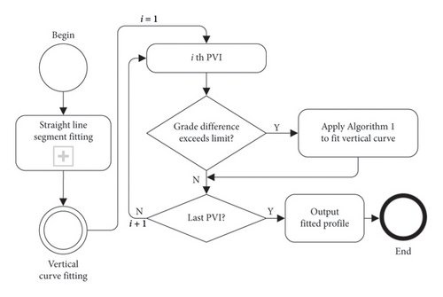
In summary, the basic procedure of the integrated fitting algorithm for both the straight-line segments and vertical curves of the longitudinal profile is illustrated in Figure 3.
4.2. GA Based on Neighbourhood Search
To address the complexities of the optimisation model described in Section 3, particularly its nonlinear objective function and multiple engineering constraints, a heuristic approach is warranted. Whilst the least squares method can provide an initial estimate for the straight-line segment gradients, it often fails to satisfy all practical constraints, such as the limits on track raising and lowering or the specific requirements for vertical curves. Therefore, this paper proposes a GA enhanced with a neighbourhood search mechanism (NSGA). GAs are well-suited for exploring complex, multimodal search spaces and can handle nonlinear objective functions and constraints effectively. The incorporation of a neighbourhood search aims to refine the solutions obtained by the GA, facilitating a more efficient convergence towards high-quality, feasible solutions by performing localised adjustments to the continuous gradient variables. This hybrid approach leverages the global search capabilities of GA with the local exploitation strength of neighbourhood search, making it a suitable strategy for the railway station track profile fitting problem.
When fitting the gradients of straight-line segments within station areas using the least squares method, two notable issues arise. First, the elevation values calculated based on the fitted gradient values may exceed the prescribed limits for raising or lowering. Second, when the algebraic difference in gradients between segments before and after a PVI is near the critical value kλ, especially when the segment lengths are short or the radii of vertical curves are large, connections between segments may incorrectly use straight-line segments instead of vertical curves, particularly when the distance between survey points is small, exacerbating the deviation.
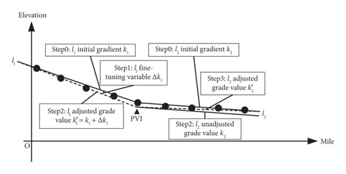
To solve the mathematical programming model, this paper proposes a GA based on neighbourhood search. The primary idea is to initialise the fitting gradient values for each gradient section kj, using the gradient values found by the least squares method. Through the algorithm’s solution mechanism, the corresponding fine-tuned gradient values Δkj are generated, thus yielding new fitting gradient values . A generic GA is employed, with special considerations given to the characteristics of neighbourhood search. This includes the design of a high-precision binary string chromosome coding scheme and the adoption of genetic operations, including single-point crossover, bit inversion mutation and the roulette wheel selection model.
4.2.1. Chromosome Design
Before the algorithm commences its search, the initial gradients of each gradient segment, denoted as kj, are set to the values obtained from the least squares fitting method. On this foundation, microadjusted gradient values Δkj within the range [−a, a] are generated through genetic operations. By making minute adjustments to the gradient of one gradient segment, corresponding subtle changes are induced in the gradient values of neighbouring segments, thereby facilitating a more rapid discovery of the optimal fitting gradient values, as illustrated in Figure 4. For instance, when a = 0.500‰, and the length of a gradient segment is 200 m, the resultant deviation at the endpoint of a gradient segment can reach up to 10 cm, which adequately satisfies the need for fine-tuning gradient values in the fitting process, as outlined in this paper.
Since the precision of the gradient change values Δkj for each segment is consistent, the total length of the string is . Here, ωj represents the length associated with the adjustment of a single gradient segment, making the total length of the initial chromosome vz(·) (where z = 1, 2, ⋯, popSize) equal to ω, with popSize being the population size. The encoding and decoding methods for the chromosomes are outlined in Algorithms 2 and 3, respectively. The notation random[0, 1] signifies generating either a 0 or 1 randomly within the interval [0, 1].
-
Algorithm 2: Binary encoding algorithm.
-
Input: Chromosome length ω.
-
Output: Chromosome vz(·).
-
Begin
-
for i = 1 to ω
-
vz(i)⟵random[0, 1];
-
end
-
Output: vz(·);
-
End
-
Algorithm 3: Binary decoding algorithm.
-
Input: Number of segments n + 1, number of encoding gene bits ωj for the gradient change value of segment j, initial gradient kj, gradient change value range [−a, a] and chromosome vz(·).
-
Output: Fine-tuned gradient value .
-
Begin
-
s⟵0, t⟵0;
-
for j = 1 to n + 1
-
s⟵t + 1;
-
t⟵t + ωj;
-
;
-
end
-
Output: Fine-tuned gradient value ;
-
End
4.2.2. Overall Algorithm Flow
GAs are characterised by parallel search capabilities, random search and probabilistic searches not bound by deterministic theories. This paper’s mechanism, based on neighbourhood search, employs a classic GA framework and customises the chromosome encoding and decoding methods according to problem characteristics. Genetic operations include single-point crossover, bit inversion mutation and selection via the roulette wheel model [24]. The essence of the algorithm is to refine the gradient values of individual straight-line segments. From each generation of the population, the best chromosome, which represents the gradient values of the straight-line segments with the smallest deviations between fitted and actual elevations, is selected. After decoding each chromosome, the integrated fitting algorithm for the longitudinal profile’s straight and curved segments, as depicted in Figure 3, is invoked. Leveraging the algorithm’s randomness and survival-of-the-fittest mechanism, an optimised fitting solution for the longitudinal profile is achieved, ensuring that the fitting results meet all model constraints whilst minimising the amounts of raising or lowering. The overall workflow of the algorithm is illustrated in Figure 5.
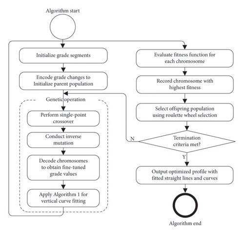
The computational complexity of the proposed GA is primarily determined by the population size, the number of generations and the complexity of the fitness function evaluation (which includes vertical curve fitting). Adjusting parameters of the GA, such as the population size or mutation rate, can improve convergence speed and efficiency. In practice, the survey data, whilst serving as input to the algorithm, do not determine the computational complexity, as its size depends on the length of the station track. Furthermore, the computational cost is negligible compared to the significant gains in fitting accuracy and the potential for substantial reductions in construction costs due to minimised track adjustments.
5. Case Study Analysis
The GA proposed in this paper, based on neighbourhood search, has been embedded into a computer program and validated for efficiency and accuracy using the centreline elevation measurement data from Track No. 7 in Area II of the Core Zone of L Railway Port in Guangxi Zhuang Autonomous Region, China. The original data were sourced from a reconstruction project at L Railway Port. The mileage spans from K537 + 980 to K540 + 100, totalling 2120 m in length, with survey points spaced 20 m apart along the rail surface, amounting to 107 survey points. The railway line is categorised as a dual-use passenger and freight line, designed for station tracks accommodating train passage. When the gradient difference between contiguous segments exceeds 4‰, it is mandatory to employ a vertical curve with a radius of 5000 m (with a challenging minimum value of 3000 m) to connect them. The shortest allowable length for any gradient section is 200 m. The throat areas, encompassing the turnout sections, are delineated from K538 + 008.53 to K538 + 229.31 and from K539 + 301.93 to K539 + 433.27. It should be noted that the stretch from K539 + 433.27 to K540 + 100 serves as the entry and exit route for the station.
For the NSGA implementation in this case study, the following parameters were employed: a population size of 10, a single-point crossover rate of 0.5, and a bit inversion mutation rate of 0.1, and the algorithm was terminated after 1000 generations. The neighbourhood search explored solutions within a ±0.5‰ gradient adjustment range for randomly selected segments in each generation.
Considering operational realities such as the ballast thickness and overhead contact line structure height, an upper limit for raising of 15 cm and a lower limit for lowering of 3 cm were set. Black diamonds in the diagram denote PVIs determined based on the engineering records, located at K38 + 320, K39 + 200, K39 + 440 and K39 + 660. The fitting results obtained using the least squares method and the NSGA are illustrated in Figure 6. As depicted in the figure, the profile generated by the NSGA avoids any overlap between PVIs and turnout areas (indicated by black dots). Additionally, the minimum grade segment length is 220 m, which exceeds the required minimum of 200 m. Notably, no track raising or lowering violations are observed. In contrast, the profile derived from the least squares method exhibits three instances of lowering violations, with a maximum violation of 5 cm.
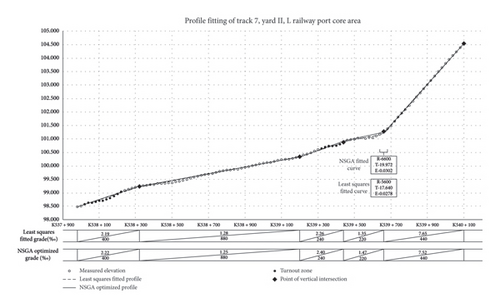
Based on the least squares fitting results for each straight-line segment, a comparison is made between the fitting outcomes from the NSGA and those from manual fitting. The relevant indicators are summarised in Table 1.
| Indices | Units | LS fitting | NSGA fitting | Manual fitting |
|---|---|---|---|---|
| Total raising amount | cm | 188 | 243 | 453 |
| Total lowering amount | cm | −67 | −37 | −4 |
| Total raising & lowering amount | cm | 255 | 280 | 457 |
| Maximum raising value | cm | 8 | 10 | 13 |
| Minimum lowering value | cm | −5 | −3 | −2 |
| Raising points | — | 48 | 62 | 79 |
| Lowering points | — | 47 | 31 | 3 |
| Maximum gradient difference | ‰ | 6.3 | 6.04 | 6.3 |
| Vertical curve radius | m | 5600 | 6600 | — |
| Length of vertical curve | m | 35.250 | 39.875 | — |
| Tangent length | m | 17.640 | 19.972 | — |
| External distance | cm | 2.78 | 3.02 | — |
| Maximum raising/lowering amount in vertical curve segment | cm | −5 | 0 | 4 |
Compared to manual fitting, the total raising or lowering amounts using the NSGA are reduced by 38.7%, indicating a closer adherence to the existing vertical profile alignment. The distribution of raising or lowering amounts in the GA fitting is relatively balanced. Constraints such as the maximum gradient limit and the maximum gradient difference comply with specified limitations, with the maximum lifting amount being 10 cm, less than the result from manual fitting. Manual fitting, adhering to the principle of ‘prefer lifting over lowering’, prioritises lifting, primarily considering factors like the thickness of the existing ballast layer and the difficulty of construction.
At PVI K39 + 660, the algebraic difference in gradients between adjacent segments surpasses the 4‰ limit, necessitating the use of a vertical curve with a radius greater than 5000 m for connection. The NSGA determines that a 6600 m-radius vertical curve is required for this section, resulting in zero lifting or lowering deviation. The length of the vertical curve is 39.875 m, the tangent length is 19.972 m, and the external offset measures 3.02 cm. Importantly, the vertical curve does not overlap with the turnout area. Conversely, manual fitting, considering the raising or lowering deviations at this location to be within an acceptable range, opts for a straight-line segment instead of a curved segment for fitting, resulting in a 4 cm deviation.
Comparing the gradient values obtained from the least squares method and the NSGA fitting, the sum of the absolute differences in gradient across segments is merely 0.45‰, as shown in Table 2. It is evident that after the NSGA fine-tunes the gradient values based on the least squares method results, it successfully avoids points of exceedance whilst yielding smaller deviations compared to manual fitting. Moreover, it effectively realises the fitting of vertical curves, highlighting the efficacy and practicality of the NSGA.
| Gradient segment | Segment 1 | Segment 2 | Segment 3 | Segment 4 | Segment 5 | |
|---|---|---|---|---|---|---|
| Fitted gradient (‰) | LS fitting | 2.19 | 1.28 | 2.26 | 1.35 | 7.65 |
| NSGA fitting | 2.22 | 1.25 | 2.40 | 1.47 | 7.52 | |
| Absolute difference | 0.03 | 0.03 | 0.14 | 0.12 | 0.13 | |
6. Conclusion
- 1.
The issue of conjugacy arising in fitting the vertical curve segments of railway station lines was addressed, and a fitting algorithm centred on the bisector vector was proposed for the integrated fitting of straight-line segments and vertical curves in longitudinal profiles. This approach optimises the calculation process and reduces the complexity of finding solutions.
- 2.
An optimisation model for fitting station line longitudinal profiles was established, accompanied by the design of a GA based on neighbourhood search. By finely adjusting the gradient values of linear segments and concurrently invoking the integrated fitting algorithm for both straight and curved segments of the longitudinal profile, a globally optimised fitting of the longitudinal profile was achieved.
- 3.
The case study demonstrates the effectiveness of the proposed model and algorithm. The approach achieves high accuracy with minimal fitting deviations, successfully integrating the optimisation of both straight-line segments and vertical curves within the longitudinal profile. Compared to manual fitting, the proposed method achieves a 38.7% reduction in track raising and lowering requirements whilst also reducing the subjectivity of manual fitting. Implementation through programming has the potential to significantly enhance both the efficiency and quality of railway station track profile fitting.
The proposed method demonstrates broad applicability for fitting longitudinal profiles of railway stations. The mathematical model, focused on minimising track adjustments under standard constraints, is generally applicable. Thus, the NSGA is suitable for various station types. It can be directly applied to small/medium stations. For larger facilities like hubs or marshalling yards, individual yard fitting and optimisation would be necessary. The fitting accuracy is inherently linked to data quality; sufficient point density is crucial for accurate curve representation and to capture the track geometry effectively. Whilst the 20 m point spacing used herein is empirically sound for typical projects, high noise levels could cause deviations. For less critical applications, sampling density might be relaxed, provided point uniformity is maintained with minimal distance variance.
Conflicts of Interest
The authors declare no conflicts of interest.
Funding
This work was supported by the National Natural Science Foundation of China (Grant No. U1834209), the Middle-Aged and Young Teachers’ Basic Ability Promotion Project of Guangxi (Grant No. 2024KY1608) and the Research Project of Guangxi Vocational College of Safety Engineering (Grant No. GAZY2023KYB005).
Acknowledgments
This study was supported by the National Natural Science Foundation of China (Grant No. U1834209), the Middle-Aged and Young Teachers’ Basic Ability Promotion Project of Guangxi (Grant No. 2024KY1608) and the Research Project of Guangxi Vocational College of Safety Engineering (Grant No. GAZY2023KYB005).
Open Research
Data Availability Statement
The data used to support the findings of this study can be obtained at the request of the corresponding author.


