An Optimization Model of Urban Transportation Travel Carbon Footprint Based on Game Theory
Abstract
To address climate change and promote green and low-carbon development, this study proposes an urban travel carbon footprint optimization method for transportation structures. Considering the environmental friendliness and efficiency of travel and combining carbon incentive policies and regret mechanisms, the travel preference model is constructed using game theory. Through the comprehensive perceived benefit function and multidimensional analysis, the effective reduction of travel carbon footprint is achieved. Taking Beijing as an example, the optimized transportation structure reduces the carbon footprint of travel by 17.17% and the total carbon emissions by 13.04%. Research has shown that to achieve the optimal carbon footprint, the green travel preference weight p1 in the multiobjective optimization model needs to be no less than 0.48, which verifies that this method can effectively alleviate the problem of transportation carbon emissions. Although this study has certain limitations in dynamic traffic demand applications, it has good practical application value for travel carbon footprint optimization under static demand conditions and contributes to the sustainable development of urban transportation and the realization of the “dual carbon” goals in China.
1. Introduction
As the global economy and society continue to evolve, environmental pollution has emerged as a focal point of research worldwide, with the call for environmental conservation growing stronger. Therefore, carbon dioxide (CO2) emissions, a primary contributor to global warming, have garnered heightened scrutiny. In response, China, a significant source of CO2 emissions [1], introduced the “dual carbon” goal in 2020. This policy aims to effectively combat climate change and foster green, low-carbon growth. The “dual carbon” initiative’s pivotal objective is to cap carbon emissions by 2030, signifying a halt in the rise of CO2 emissions, and to endeavor for carbon neutrality by 2060 [2]. Achieving carbon neutrality entails counterbalancing CO2 emissions through diverse strategies to reach a state of net-zero emissions.
By the “Strategy to Reduce Greenhouse Gas Emissions from Inland Transport,” ratified by the United Nations Inland Transport Committee (ITC) in February 2024, it has been revealed through data that the transportation sector is responsible for nearly 23% of the global annual greenhouse gas emissions, positioning it as a key contributor to carbon emissions [3]. The strategy underscores the significance of public transportation and advocates for a target of net-zero emissions for greenhouse gases within the transportation sector by the year 2050. In China, it is observed that urban transportation systems not only facilitate a substantial daily passenger turnover but also contribute significantly to greenhouse gas emissions. Low carbon and green transportation have become increasingly popular demands, so how to effectively control the carbon emissions of urban transportation systems has become the key to achieving net-zero emissions in transportation. Among them, the transformation and optimization of urban transportation structures stand out as pivotal measures in advancing green transportation. Many scholars adjust the overall structure of urban transportation to achieve a reduction in the total carbon emissions of transportation [4–6]. Nonetheless, considering only reducing total carbon emissions may inevitably lead to a reduction in total traffic volume, which to some extent reduces transportation efficiency. The concept of the carbon footprint, introduced as a significant metric for CO2 emissions in 1990, emphasizes the enhancement of carbon emission reduction efficiency [7]. The travel carbon footprint is defined by the emissions produced per kilometer traveled by an individual, offering a more accurate representation of low-carbon travel efficiency. Due to the diverse travel preferences of different groups in the urban transportation structure, there is currently limited research on optimizing the overall structure of urban transportation considering subjective preferences. Therefore, starting from individual travel choices, this study considers two aspects of travel environmental friendliness and travel efficiency and uses game theory to analyze the macro travel-biased weight problem. It is then introduced into the urban transportation structure optimization model to explore a new method for optimizing the travel carbon footprint under the overall system. This effectively alleviates the problem of urban transportation CO2 pollution and provides theoretical research support for China to achieve the “dual carbon” goal.
2. Literature Review
In the development process of urban transportation, green transportation and sustainable development have always been the focus of academic attention. With the acceleration of urbanization, the number of cars has surged, leading to traffic congestion and a decline in air quality, posing a threat to the sustainable development of cities [8–10]. Therefore, how to reduce the negative impact on the environment while ensuring convenient transportation has become an urgent problem to be solved.
Among them, the monitoring and governance of carbon emissions from transportation is of paramount importance in promoting the sustainable development of urban transportation [11]. For example, Ji et al. [12] studied the monitoring method of carbon emissions from Shanghai’s highway transportation considering electric vehicles. Based on summarizing vehicle emission measurement methods, Mądziel [13] studied the accuracy of different emission simulation software. Zong and Yue [14] analyzed the impact of carbon emissions generated by vertical transportation oscillations on environmental pollution. There are other studies on carbon emission monitoring, including models for measuring traffic emissions and pollution in high-speed environments [15], methods for calculating traffic carbon emissions in complex urban building structures [16], and carbon emission assessment methods combining gray cubic index smoothing models [17]. In addition, in recent years, while exploring monitoring algorithms, research on optimizing the governance of transportation carbon emissions has also emerged one after another. The efficient and sustainable urban transportation structure is currently a hot topic in the research of emission reduction plans [18, 19]. Tsoi et al. [20] studied the overall traffic structure optimization considering environmental pollution in the context of electric vehicles. Qiang et al. [4] constructed a carbon emission optimization model that considers energy efficiency to optimize urban transportation structure. Lin andWang [21] explored the specific carbon emission reduction effects of transportation structure adjustment under different situations. Therefore, establishing a reasonable and superior multiobjective optimization model has become an important way to control and optimize transportation carbon emissions [22, 23].
However, in the existing multiobjective optimization research on urban transportation structure, most only consider objective factors such as traffic turnover [18], traffic carbon emissions [20], and traffic energy consumption [4] and fit and add them through dimensionless transformation, thus ignoring the influence of residents’ subjective perception on the weights of different objective indicators. Moreover, in the research field of residents’ subjective travel choices, scholars have focused more on determining the probability of different travel mode choices and have rarely further combined it with overall structural optimization [24]. Among them, Mishra et al. [25] used the comprehensive intuitionistic fuzzy proximity coefficient to study the selection of urban transportation travel plans. Zhou et al. [26] used a latent class nested logit model to analyze the travel mode choices of urban tourists.
In actual travel, due to factors such as carbon incentive policies and travel regret psychology, conventional logit models and other analysis methods have low efficiency in dealing with this nonlinear system [25, 26]. To improve the stability and effectiveness of the overall model, this paper introduces the idea of game theory, treating the allocation of indicator weights in multiobjective models as a game process, and proposes a new carbon footprint optimization method that combines game theory and multiobjective modeling ideas. Compared with the existing achievements mentioned above, the method proposed in this paper not only considers the subjective perception of residents’ travel but also replaces the conventional total carbon emission indicators [4, 20, 21], taking carbon footprint as the main influencing indicator and focusing on improving carbon emission reduction efficiency, thereby reducing the possibility of comprehensive traffic reduction in the optimization results, which has more practical application value. This study aims to explore the feasibility of game theory methods and multiobjective function joint modeling, analyze the impact of individual subjective preferences on overall transportation mode optimization, discuss the necessary conditions for achieving optimal travel carbon footprint under sustainable development goals, and provide a theoretical basis for achieving China’s “dual carbon” goals.
3. Methodology
3.1. Model Architecture
To address the “dual carbon” goal and cater to the need for sustainable transportation, this study zeroes in on the comprehensive structural refinement of urban transit systems. It presents a carbon footprint optimization model tailored for urban transportation, which thoroughly accounts for residents’ subjective preferences in travel decisions, ensuring a closer alignment with real-world scenarios. The model aims to integrate the characteristics and advantages of different transportation modes while maintaining travel efficiency and minimizing travel carbon footprint as much as possible. Considering the complexity and uncertainty of urban transportation, to ensure the accuracy and effectiveness of the method, the model only considers the five major transportation modes in the city, namely, private car (x1), taxi (x2), bus (x3), rail transit (x4), and bicycle (x5). Due to the different subjective travel biases of different resident groups in the optimization model, a travel choice distribution model is constructed using game theory to address the two subjective preferences of travel environmental friendliness and travel efficiency. The game model combines the travel satisfaction-regret mechanism and considers the impact of different urban carbon incentive policies, thereby improving the stability and objectivity of the model. Finally, this study sets constraints based on four dimensions: demand, resource, space–time, and scale. Based on the proportion of environmental and efficiency preferences, the carbon footprint of travel is optimized to obtain the optimal urban transportation structure. This structure is instrumental in steering urban transport evolution in the direction of sustainable progress. The specific architecture of the model is shown in Figure 1.
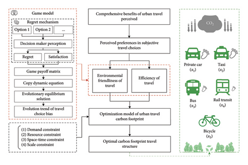
From Figure 1, it can be seen that the method proposed in this article is mainly based on a multiobjective optimization model, introducing game theory methods to determine the weights of multiobjective functions, achieving maximum travel perception benefits, and thus obtaining the optimal carbon footprint travel structure.
3.2. Optimization Model of Urban Residents’ Travel Carbon Footprint
This section will provide a detailed introduction to the calculation process of the urban transportation travel carbon footprint optimization model proposed in this article.
3.2.1. Objective Function
3.2.1.1. Environmental Friendliness of Travel
3.2.1.2. Efficiency of Travel
To improve the stability of the model, equation (1) is used to perform dimensionless processing on T, resulting in T∗, which is expressed as the degree of travel utility per person per kilometer (0∼1), reflecting the efficiency of travel.
3.2.1.3. Comprehensive Objective Function
3.2.2. Constraint Conditions
This article constructs the constraints of a mathematical model from four dimensions: demand constraints, resource constraints, space–time constraints, and scale constraints.
3.2.2.1. Demand Constraints
3.2.2.2. Resource Constraints
3.2.2.3. Space–Time Constraints
3.2.2.4. Scale Constraints
3.2.3. Multiobjective Optimization Model
3.3. Evolutionary Game Model of Urban Travel Choice Preferences Under the Goal of Dual Carbon
Travel perception preference weight refers to the subjective psychological bias that arises during an individual’s travel process due to external and personal circumstances. For example, if travelers believe that travel efficiency is more important than low-carbon environmental protection, then p2 > p1, and vice versa. Its value range is mainly determined by the subjective perception of individual travel and the importance judgment of different choices. Therefore, it has uncertainty and dynamic variability. Because this dynamic perception selection process is a game decision-making process [29], and the two choices tend to be relative, this paper uses game theory to study the subjective choice bias weights of residents’ travel, providing a basis for solving the optimization model of urban travel carbon footprint. In addition, due to the dynamic behavior characteristics of travel choice decisions, evolutionary game theory is more suitable for the research content of this paper than traditional Nash equilibrium or discrete choice models.
In the urban transportation, there may be two travel biases: green travel or efficient travel, and different people have various acceptance of environmental protection concepts. Assuming that the decision to adopt green travel is G, the decision to adopt efficient travel is E, the acceptance of environmental protection ideas is recorded as IA, and the nonacceptance of environmental protection ideas is recorded as IR. Assuming there are two types of undifferentiated groups I and II, they have reached a consensus on noncooperative behavior in the large-scale decision-making of green and efficient travel, forming a collective convergence behavior. If both travel groups I and II lean toward green travel, the game benefits are recorded as (A, A). If both travel groups I and II lean toward efficient travel, the game benefits are recorded as (B, B). If travel group I leans toward green travel and travel group II leans toward efficient travel, the game benefits are recorded as (C, D). If travel group I leans toward efficient travel and travel group II leans toward green travel, the game benefits are recorded as (D, C).
- •
Decision 1 (G, IA): leaning toward green travel and accepting environmental protection ideas and will receive additional environmental policy and psychological benefits, denoted as θ + α.
- •
Decision 2 (G, IR): leaning toward green travel and rejecting environmental protection ideas and will receive additional environmental policy benefits and psychological costs, denoted as θ − α.
- •
Decision 3 (E, IA): leaning toward efficient travel and accepting environmental protection ideas and will receive additional psychological costs, denoted as −α.
- •
Decision 4 (E, IR): leaning toward efficient travel and rejecting environmental protection ideas and will receive additional psychological benefits, denoted as +α.
In summary, based on game theory, an analysis is conducted on the travel benefits of urban residents, taking into account the mechanism of travel regret and the benefits of low-carbon policies. The game payoffs matrix M4×4 with preferences toward urban travel choices is constructed, as shown in Table 1.
| Decisions | (G, IA) | (G, IR) | (E, IA) | (E, IR) |
|---|---|---|---|---|
| (G, IA) | (A + θ + α, A + θ + α) | (A + θ + α, A + θ − α) | (C + θ + α, D − α) | (C + θ + α, D + α) |
| (G, IR) | (A + θ − α, A + θ + α) | (A + θ − α, A + θ − α) | (C + θ − α, D − α) | (C + θ − α, D + α) |
| (E, IA) | (D − α, C + θ + α) | (D − α, C + θ − α) | (B − α, B − α) | (B − α, B + α) |
| (E, IR) | (D + α, C + θ + α) | (D + α, C + θ − α) | (B + α, B − α) | (B + α, B + α) |
According to equation (27), if y1 ≠ 0, then , and it is obvious that y2 = 0; On the contrary, when y2 ≠ 0, then y1 = 0. Similarly, according to equation (28), it can be concluded that y3 and y4 must have a value of 0. Based on the actual transportation selection environment, it can be found that Decision 2 and Decision 3 are relatively disadvantaged strategies. Therefore, in real life, their evolutionary game trend will gradually develop toward Decision 1 and Decision 4 and tend to stabilize. To obtain a stable trend toward the evolution of urban travel choices, the matrix M4×4 was simplified, considering only Decision 1 and Decision 4. The simplified game payoffs matrix H2×2 is shown in Table 2.
| Decisions | (G, IA) | (E, IR) |
|---|---|---|
| (G, IA) | (A + θ + α, A + θ + α) | (C + θ + α, D + α) |
| (E, IR) | (D + α, C + θ + α) | (B + α, B + α) |
Let dz1(t)/dt = 0 and dz2(t)/dt = 0, then there are clearly three sets of evolutionary equilibrium solutions, two of which are and . These two sets of solutions are too ideal and have a low degree of conformity with the actual traffic situation. Therefore, this article mainly considers the equilibrium state of the third set of solutions. According to equations (32) and (33), it can be obtained and . Among them, α is reduced in the derivation. Due to 0 < z1, z2 < 1, the equilibrium conditions are obtained as follows: Condition 1: C + D − A − B > 0, B − C < θ, D − A > θ and Condition 2: C + D − A − B < 0, B − C > θ, D − A < θ.
If is substituted into equation (34), then . According to the stability rule of game theory [31], if and only when , tends to a stable state, which can be divided into the following conditions: (1) C + D − A − B > 0, B − C < θ, D − A > θ; (2) C + D − A − B > 0, B − C > θ, D − A < θ; (3) C + D − A − B < 0, B − C > θ, D − A > θ; and (4) C + D − A − B < 0, B − C < θ, D − A < θ.
Comparing equilibrium Conditions 1 and 2, it is found that the game evolution model has evolutionary equilibrium solutions and that conform to the general meaning of transportation, only when C + D − A − B > 0, B − C < θ, and D − A > θ are satisfied. Thus, the preference weights for green travel and efficient travel in the multiobjective optimization model of this article can be calculated, i.e., and .
4. Case Analysis
To verify the effectiveness of the method proposed, a case study was conducted on the behavior of residents in the central urban area of Beijing. In this case, with 2020 as the current year and 2030 as the planning year, we aim to optimize the transportation structure and carbon footprint of the central urban area of Beijing. By referring to the overall plan of Beijing and relevant literature [32], the current traffic situation and planning requirements in the central urban area of Beijing are obtained as follows.
In 2020, the construction land in the central urban area of Beijing was approximately 778 km2, with a permanent population of 10.9890 million people and a total daily travel volume of 36.1900 million people. The daily travel distance was 11.1 km, and the daily travel rate was 3.29 times per person. According to the plan, the construction land scale of the central urban area in 2030 is 832 km2, with an equivalent urban radius R of 16.28 km. Based on the land area, the estimated population size is around 11.7517 million people, and the daily travel rate is about 3.58 times per person. Therefore, the planned annual daily travel volume is 42.0711 million people. Excluding the travel volume of walking and other small-scale transportation modes, as referenced in reference [32], their proportion is approximately 32.89%. The planned annual daily travel volume N of the five mainstream urban passenger transportation modes discussed in this article in the central urban area of Beijing is about 28.2339 million people. Based on the overall plan of Beijing, the urban per capita road area LS is set at 10 m2/person by 2030. Assuming that the ideal average travel time t in Beijing is 0.67 h and the ideal average travel distance r is 11.6 km, the total turnover demand TN is 327.51 million people·km. According to Carlsson-Kanyama and Linden [33] and the current energy situation in China, the upper limit of energy consumption for passenger transportation in Beijing is 18.1MJ/d (Mega Joule/day). Therefore, the daily energy carrying capacity EN of Beijing’s passenger transportation system in 2030 is 2.13 × 10⁸ MJ. Through the current situation investigation, it was found that the parking rate δ in Beijing is about 0.78. Based on the number of planned parking spaces, the total planned parking area M is 5.06 × 10⁷m2. Taking 80% of the travel time demand as the tolerable maximum travel time, ts is about 1.05 h, and the unit time value vot is 30.97 yuan/h. According to relevant references and survey status, the relevant parameter settings of the model in this article are shown in Table 3. Among them, referring to the carbon footprint data of different vehicle models published by the Ecological China website and relevant literature [7], the carbon emission coefficients of different transportation modes can be obtained. However, although transportation modes x1 and x2 are two different modes of transportation, they belong to the same category of vehicles. Therefore, by combining the average passenger capacity coefficient Si, the ei of both can be inferred. For example, according to statistics, the carbon footprint of a car is 259.7 g/vehicle, so the carbon emission coefficient of x1 is e1 = 259.7/S1.
| Parameters | Transportation modes | Units | References | ||||
|---|---|---|---|---|---|---|---|
| Private car | Taxi | Bus | Rail transit | Bicycle | |||
| x1 | x2 | x3 | x4 | x5 | |||
| ei | 92.75 | 129.85 | 30.40 | 24.70 | — | g/(person·km) | [7] |
| ki | 0.0237 | 0.0144 | 0.0429 | 0.0893 | 0.0171 | — | [34] |
| εi | 1.82 | 1.34 | 1.00 | 1.00 | 0.63 | — | [35] |
| Oi | 14.3 | 21.0 | 2.0 | 4.0 | 1.5 | Yuan | [35] |
| μi | 0.291 | 0.291 | 0.170 | 0.113 | 0.021 | Yuan/(person·km) | [35] |
| ci | 8.9 | 5.7 | 1.1 | 1.2 | 3.6 | — | [36] |
| ri | 14.0 | 9.1 | 10.7 | 17.4 | 2.9 | km | [32] |
| lsi | 15.00 | 18.75 | 1.50 | 0.50 | 7.40 | m2/person | [37] |
| Si | 2.8 | 2.0 | 52.0 | 410.0 | 1.0 | Person/vehicle | [38] |
| Ai | 13.25 | 13.25 | 45.60 | — | 1.20 | m2 | [38] |
| ti | 0.674 | 0.433 | 0.998 | 1.119 | 0.382 | h | [32] |
| vi | 33.0 | 30.0 | 26.0 | 35.6 | 10.3 | km/h | [32] |
| γi | 1.46 | 1.82 | 0.23 | 0.21 | — | MJ/(person.km) | [27] |
| 69.97 | 3.79 | 66.84 | 115.95 | 13.29 | Million people·km | [32] | |
| 101.69 | 11.37 | 133.69 | 253.64 | 15.22 | Million people·km | [32] | |
According to the equilibrium condition obtained in Section 3.3 and concerning reference [39], the range of model parameters can be calibrated as follows without losing generality: A, B ∈ {1, 2, 3}, C, D ∈ {4, 5, 6}, corresponding to the corresponding return levels of low, medium, and high, respectively. Among them, if the subsidy income generally does not exceed the regular income, then θ ∈ (0, 1). Based on Table 3 and the relevant travel situation in Beijing, it can be concluded that A is Medium (2), B is Low (1), C is High (6), and D is Medium (5). Due to the rich carbon incentive policies in Beijing, let θ = 0.8. Therefore, the evolution trend of travel choices in Beijing is shown in Figure 2.

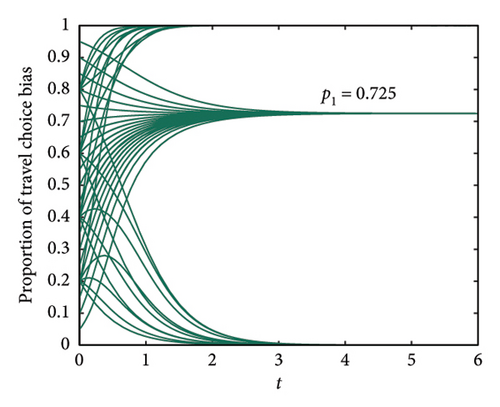
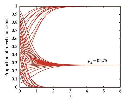
As shown in Figure 2, the preference weights for travel choices are 0.725 and 0.275, respectively. According to equation (7) and reference [28], combined with the survey status, the weights for turnover efficiency, travel economy, and travel comfort are 0.18, 0.23, and 0.59, respectively. Due to multiple normalization processes in the article to ensure the reliability of the model, in order to clarify the objective functions of each stage of the model, the corresponding coefficients are given in Table 4. Taking C∗ as an example, , and the same applies to others.
| Parameters | x1 | x2 | x3 | x4 | x5 |
|---|---|---|---|---|---|
| I(C∗) | −3.6340 | −6.7839 | 1.6596 | 2.1435 | 4.2406 |
| −1.7871 | −2.3968 | −0.5284 | 2.5134 | −2.2198 | |
| −2.9168 | −5.6985 | 1.3427 | 2.3125 | −1.2160 | |
| 5.4508 | 2.6369 | −1.4081 | −1.3201 | 0.7903 | |
| I(T∗) | 5.2656 | −1.2341 | −2.3960 | −0.1776 | −1.3060 |
| I(Z) | −1.1866 | −5.2577 | 0.5443 | 1.5052 | 2.7153 |
Among them, by importing the values of each parameter in Table 3 into equation (17), the specific values of the constraints for solving the problem in this paper can be obtained. Moreover, since the normalization equations (1) and (2) require obtaining the MAX and MIN of each indicator under these constraints, each stage of the model is equivalent to solving an optimization problem. Table 4 directly shows the coefficient situation of the normalized objective function. According to equation (8) and Table 4, the final objective function is obtained as .
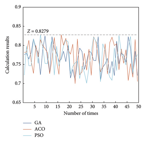
Because the problem studied in this article is a fractional programming problem, and using heuristic intelligent algorithms to solve such problems is prone to getting stuck in local optima, this article uses the Dinkelbach’s Transform [40] to transform fractional programming into linear programming for solution. The Dinkelbach’s Transform is a mature method for solving fractional programming problems. Its core idea is to iteratively transform the division problem into a subtraction problem, that is, to transform f(x)/g(x) into f(x) − ζg(x) and iteratively update the value of ζ to find the global optimal solution. In practical calculations, due to the complexity of the model, MATLAB programming was used to simulate the iterative process and obtain the optimal solution Max Z = 0.8279. The daily traffic turnover of the five transportation modes under this optimal solution are 69.97, 3.79, 66.84, 233.14, and 13.29 million people·km. Based on equations (9) and (10) and their related descriptions, it can be inferred that the travel volume is xi/ri, thus obtaining the daily traffic volume for each mode of transportation after optimization. And, the total traffic volume is 29.6428 million people per day. In combination with the status quo of the investigation before optimization, the changes in the urban travel structure before and after optimization are obtained, as shown in Table 5.
| Transportation modes | x1 | x2 | x3 | x4 | x5 |
|---|---|---|---|---|---|
| Daily traffic turnover (million people·km) | 69.97 | 3.79 | 66.84 | 233.14 | 13.29 |
| Daily traffic volume (million people) | 4.9979 | 0.4165 | 6.2467 | 13.3989 | 4.5828 |
| Partaking rate after optimization (%) | 16.86 | 1.41 | 21.07 | 45.20 | 15.46 |
| Partaking rate before optimization (%) | 24.37 | 3.16 | 24.05 | 32.82 | 15.60 |
| Proportional change (%) | −7.51 | −1.75 | −2.98 | 12.38 | −0.14 |
To avoid travel calculation errors in iterative solving using the Dinkelbach’s Transform in this article, three commonly used heuristic algorithms, genetic algorithm (GA) [41], ant colony optimization (ACO) [42], and particle swarm optimization (PSO) [43], were selected to verify the accuracy of the results. The results of 50 local optima obtained by solving 50 random initial solutions using three algorithms are shown in Figure 3(a). Among them, all solutions are less than or equal to 0.8279, and some initial solutions can converge to Z = 0.8279, thus verifying that Z = 0.8279 is the global maximum value.
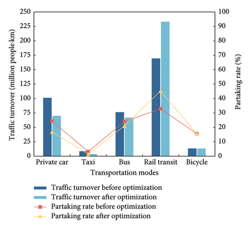
According to the partaking rates of transportation modes before optimization in Table 5 and the parameter ri regarding travel distance in Table 3, the traffic turnover volumes before optimization are 101.14, 8.52, 76.28, 169.28, and 13.41 million people·km, respectively. The comparison chart of turnover and partaking rate before and after optimization is shown in Figure 3(b). From the graph, it can be seen that the proportion of rail transit travel has significantly increased after optimization, by 12.38%.
By combining equation (3) with traffic turnover before and after optimization, the average travel carbon footprint and total carbon emissions of Beijing before and after optimization can be obtained. Among them, the carbon footprint of Beijing’s travel was 46.08 g/(person·km) before optimization and 38.17 g/(person·km) after optimization, a reduction of 17.17%. The total daily carbon emissions were 16,987.333 t (metric tons) before optimization and 14,772.343 t after optimization, a decrease of 13.04%.
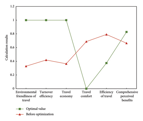
Based on the travel structure before and after optimization, the optimization degree of different indicators is obtained using equations (1)–(8), as shown in Table 6. A comparison chart of different indicators before and after optimization is drawn, as shown in Figure 4. It can be seen from this that optimized travel has significantly improved environmental friendliness, economy, and turnover efficiency. Although the travel comfort has decreased to a certain extent, the overall perceived benefits of travel have been improved, with an optimization degree of 0.1640. This verifies that the method proposed in this article ensures travel efficiency to a certain extent while significantly reducing the carbon footprint of travel, effectively alleviating CO2 pollution, and providing a theoretical basis for the green development of urban transportation.
| Parameters | C∗ | T∗ | Z | |||
|---|---|---|---|---|---|---|
| Optimal value | 1.0000 | 1.0000 | 1.0000 | 0.0000 | 0.3742 | 0.8279 |
| Before optimization | 0.3282 | 0.4184 | 0.3636 | 0.6876 | 0.7913 | 0.6639 |
| Optimized degree | 0.6718 | 0.5816 | 0.6364 | −0.6876 | −0.4171 | 0.1640 |
5. Discussion
To further study the issues of environmental pollution and carbon footprint optimization, this article will discuss and analyze the following aspects, highlighting the practical application value of the model.
5.1. Stability Analysis of Low-Carbon Travel Structure Under Different Carbon Incentive Policies
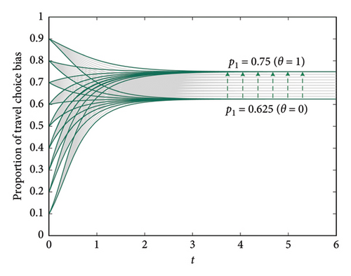
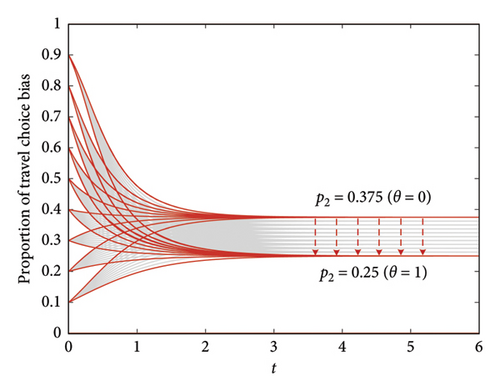
Under the “dual carbon” goal, different cities in China are paying increasing attention to carbon emission control and have formulated different carbon incentive policies, such as carbon credits and carbon neutrality subsidies. So, under different carbon incentive policies, what kind of stable structure does urban transportation exhibit? This article uses the data from Section 4 for further analysis, taking θ as 0∼1 for discussion: the larger the θ is, the greater the corresponding carbon incentive policy intensity will be. Through programming and simulation, the evolution trend of travel preferences in Beijing under different carbon incentive policies was obtained, as shown in Figure 5. Among them, Figure 5(a) shows the evolution of the weight of green travel in the comprehensive travel perceived benefit when θ varies from 0 to 1; Figure 5(b) shows the evolution of the weight of efficient travel in the comprehensive travel perceived benefit when θ varies from 0 to 1. It can be seen from this that the greater the carbon incentive policy, the higher the degree of inclination toward green travel. Also, when θ is 0, p1 = 0.625 and p2 = 0.375 and when θ is 1, p1 = 0.75 and p2 = 0.25.
Using the carbon footprint optimization model, the urban travel structure with θ between 0 and 1 was calculated. It was found that the optimal travel structure remained unchanged, as shown in Table 5. Under this structure, there is the optimal travel carbon footprint, presenting a low-carbon travel structure. However, by analyzing the values of the objective function under different carbon incentive policies, it was found that the value of the comprehensive perceived benefit Z is not constant but shows a linear change trend, as shown in Figure 6.
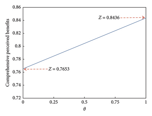
According to Figure 6, it can be seen that when θ = 0, the comprehensive perceived benefit Z is 0.7653 and when θ = 1, the comprehensive perceived benefit Z is 0.8436. Among them, as θ tends toward 1, the value of Z increases, indicating a higher degree of recognition of the travel structure. Therefore, the greater the intensity of carbon incentive policies, the higher the stability of low-carbon travel structure in urban transportation.
5.2. Parameter Analysis of Residents’ Travel-Biased Game Model Under Optimal Carbon Footprint Objective
To meet the needs of sustainable transportation development, it is always necessary to maintain the goal of prioritizing low-carbon transportation in urban planning. This section will explore the parameter changes in the residents’ travel-biased game model based on the optimal carbon footprint. To achieve the optimal travel carbon footprint, urban transportation needs to stabilize toward the low-carbon travel structure. Using the carbon footprint optimization model constructed in this article, the perceived benefits and changes in travel structure of green travel preference weight p1 between 0 and 1 were studied, as shown in Figure 7. Combining equation (8), Figure 7(a) shows the changing trends of indicators C∗, T∗, and Z under different p1, which, respectively, represent environmental friendliness of travel, efficiency of travel, and comprehensive perceived benefits. Figure 7(b) highlights the optimal travel structure under different p1, showing the composition of traffic turnover for each mode of transportation. Thus, according to Figure 7, it can be concluded that when p1 is 0.3∼0.5, the stable state of its travel structure changes from the efficient to the low-carbon travel structure.
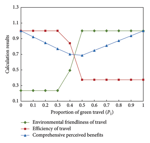
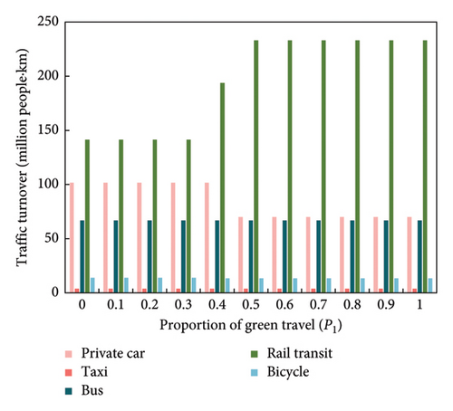
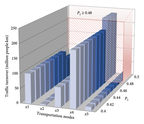
From Figure 7(b), it can be seen that there is a stable point in p1 between 0.4 and 0.5, which stabilizes the travel structure toward low-carbon travel and achieves the goal of the lowest travel carbon footprint. Through calculation and analysis, the optimal travel structure composition of p1 between 0.4 and 0.5 after refinement was obtained, as shown in Figure 8. From Figure 8, it can be observed that the stable point of p1 is at 0.48. When p1 ≥ 0.48, the travel structure is low carbon, which meets the requirements of optimizing travel carbon footprint and reduces travel carbon emissions.
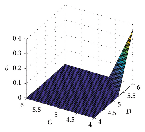
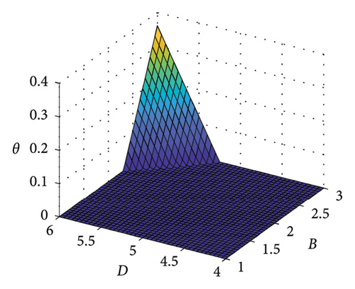
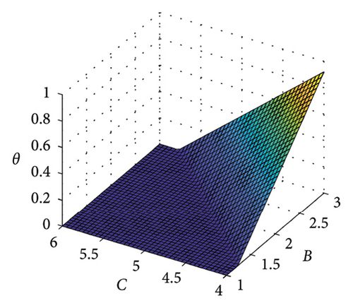
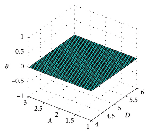
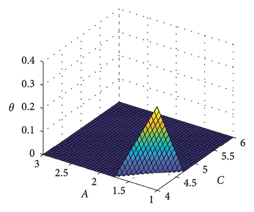
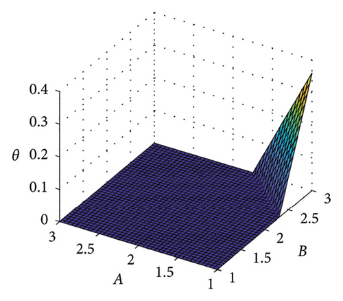
According to the game model in Section 3.3, it can be concluded that when (θ + C − B)/(C + D − A − B) ≥ 0.48, the travel structure satisfies the optimal carbon footprint. Therefore, the parameter analysis of the game model for achieving the optimal carbon footprint target is shown in Figure 9. Based on the current data in Section 4, under the condition of fixed values for two parameters, we explored the range of values for the other three variables that meet the minimum travel carbon footprint target. (i.e. the area above the color plane). From Figure 9, it can be seen that the larger the value of A, the better; the smaller the value of B, the better; the larger the value of C, the better; and the smaller the value of D, the better. Among them, the value of θ is very important for the stability of the low-carbon travel structure, and cities should continuously promote carbon incentive policies to promote sustainable development of urban transportation.
6. Conclusion
As one of the main sources of carbon emissions, the transportation sector actively deals with urban traffic pollution, which can effectively respond to climate change and promote green and low-carbon development. This study focuses on improving urban transportation structure, analyzes individual travel preferences through game theory, and proposes a new method for optimizing travel carbon footprint. The study considers two aspects of travel environmental friendliness and travel efficiency, combined with factors such as carbon incentive policies and regret mechanisms. It constructs an evolutionary game model for travel choices, which provides a theoretical basis for determining the weight of travel preferences. By integrating the benefits of both parties to obtain a comprehensive perceived benefit function, this study combines dimensions of demand, resource, space–time, and scale to explore the urban transportation structure that can effectively reduce the travel carbon footprint. The model in this paper has a certain degree of universality. Even for some cities without rail transit, the model can be solved by flexibly adding constraints.
Taking Beijing as a case study, the analysis and discussions show that the optimized transportation structure reduced the carbon footprint of travel by 17.17% and the total carbon emissions by 13.04%. To achieve the goal of optimal carbon footprint and stabilize the transportation structure toward low-carbon travel, the green travel preference weight p1 in the multiobjective optimization model needs to be no less than 0.48. This indicates that cities need to continuously improve carbon incentive policies, such as improving public transport priority policies, carbon points reward policies, congestion charging policies, and new energy vehicle subsidy policies, to meet the needs of urban travel to reduce the carbon footprint. The method proposed in this article not only fully considers the subjective psychology of residents and calculates the optimized traffic structure positively but also effectively deduces the necessary conditions for achieving the optimal carbon footprint in reverse, which has important practical application value. This contributes to the sustainable development of urban transportation in China and the implementation of the “dual carbon” goals.
Conflicts of Interest
The authors declare no conflicts of interest.
Author Contributions
Xiaoyu Wu: conceptualization, methodology, data curation, supervision, and writing the original draft; Aiguo Lei and Lishuang Bian: reviewing and editing.
Funding
This work was supported by the National Natural Science Foundation of China (51178157); the High-Level Project of the Top Six Talents in Jiangsu Province (JXQC-021); and the Key Science and Technology Program in Henan Province (182102310004).
Appendix A: The Summary Table of Variables
Table A1 summarizes the meanings and units of all variables in the carbon footprint optimization model for urban travel in this article.
| Variables | Meanings | Units |
|---|---|---|
| xi | Daily turnover of different transportation modes | People·km |
| Cf | Average travel carbon footprint | g/(person·km) |
| Variable Cf that has undergone dimensionless processing | — | |
| C∗ | Low-carbon level of travel per person per kilometer (0∼1) | — |
| ei | Carbon emission coefficient of transportation mode xi | g/(person·km) |
| T1 | Average transportation capacity of traffic | — |
| T2 | Average travel cost of traffic | Yuan/(person·km) |
| T3 | Average travel comfort level of traffic | — |
| ki | Transportation turnover coefficient of transportation mode xi | — |
| Tt | Average time cost of travel | Yuan/(person·km) |
| Tu | Average usage cost of travel | Yuan/(person·km) |
| Te | Average external cost of travel | Yuan/(person·km) |
| vot | Per capita unit time value of urban residents | Yuan/h |
| εi | Time value coefficient of transportation mode xi | — |
| vi | Average operating speed of transportation mode xi | km/h |
| Oi | Average transportation price per person using xi | Yuan |
| ri | Average travel distance of transportation mode xi | km |
| μi | External cost per unit distance generated by each person using xi | Yuan/(person·km) |
| ci | Comfort coefficient of transportation mode xi | — |
| Variable T1 that has undergone dimensionless processing | — | |
| Variable T2 that has undergone dimensionless processing | — | |
| Variable T3 that has undergone dimensionless processing | — | |
| ωi | Weights of turnover efficiency T1, travel economy T2, and travel comfort T3 | — |
| T∗ | Degree of travel utility per person per kilometer (0∼1) | — |
| pi | Travel perception bias weight of C∗ and T∗ | — |
| Z | Comprehensive perceived benefits of transportation | — |
| TN | Total travel demand turnover | People·km |
| N | Daily travel demand | People/day |
| r | Average travel distance | km |
| λ | Error range (generally taken as 5%) | — |
| lsi | Per capita dynamic land area of transportation mode xi | m2/person |
| LS | Per capita road area occupied by the city in the planning year | m2/person |
| δ | Parking rate of the city (generally taken as 0.5∼0.8) | — |
| Si | Average number of passengers carried by transportation mode xi | People/vehicle |
| Ai | Average parking area of transportation mode xi | m2 |
| M | Total parking area of the target year’s urban planning | m2 |
| t | Average travel time of urban residents in the planning year | h |
| R | Equivalent radius of the city in the planning year | km |
| ti | Average travel time of transportation mode xi | h |
| ts | Average maximum travel time that urban residents can tolerate | h |
| γi | Energy consumption factor of transportation mode xi | MJ/(person·km) |
| EN | Upper limit of the total energy consumption of urban transportation | MJ |
| Lower limit of the development scale of transportation mode xi | Person·km | |
| Upper limit of the development scale of transportation mode xi | Person·km |
Open Research
Data Availability Statement
The data that support the findings of this study are available from the corresponding author upon reasonable request.


