Research on Vehicle Following and Overtaking Safety Distance Models Considering Trust Level of Driving
Abstract
To investigate the influence of drivers’ cognitive differences on the vehicle driving process, this paper focuses on the mechanism of drivers’ cognition of vehicles, roads, and environments. Existing studies of vehicle following and overtaking usually set the driver reaction time, vehicle braking deceleration, and acceleration as fixed values, ignoring the individual differences of drivers and their influence by road conditions. Therefore, firstly, the concept of “trust level of driving” is proposed and real vehicle tests and simulator tests for different drivers and different working conditions are designed to quantify the trust level of driving. Addressing the limitations of existing car-following and overtaking models, a safety distance model and a two-way dual-lane highway overtaking model are developed based on trust level of driving. Finally, the driving simulator is used to create scenarios, and the effectiveness of the model is verified. The safe vehicle distance and overtaking distance required by drivers with different trust levels of driving are obtained, and their applicability is explained. In this study, a more accurate and humanized model of safe distance and overtaking was developed to help address driver cognitive deficits and improve traffic safety.
1. Introduction
At present, the ownership of cars in the market and road construction levels are rapidly increasing, leading to a significant surge in traffic volumes. This surge has brought issues of great concern, including traffic safety, road congestion, energy loss, and environmental pollution, to the forefront [1–4]. Research has demonstrated that human factors, vehicle-related issues, road conditions, and environmental factors contribute to traffic accidents in proportions of 59.7%, 10.1%, 17.4%, and 12.8%, respectively [5]. Notably, human factors are the primary cause of traffic accidents. This can be attributed to the multifaceted roles that drivers assume, acting as both experiencers and decision makers within the closed-loop system involving humans, vehicles, and roads. These roles come with complexity and uncertainty. Hence, the investigation of the driver’s cognitive mechanisms related to vehicles, roads, and the environment serves as an effective approach to avoiding traffic accidents.
Drivers’ behavior primarily falls into three categories: following, lane changing, and overtaking. Each of these behaviors has corresponding safety boundaries, commonly referred to as safety distances. Extensive research has been conducted by scientists worldwide to study safety distances. Drivers’ diverse perceptions of vehicles, roads, and their surroundings are influenced by factors such as gender, age, familiarity with the environment, among others [6]. Therefore, exploring the cognitive properties of drivers is the basis for realizing the humanization and personalization of intelligent vehicles. In terms of the car’s perception of the driver, different driving styles are categorized as aggressive, general, and moderate [7]. Certain scholars have developed improved algorithms to establish a model for recognizing driving styles, enabling more accurate identification of driver styles [8–10]. The safety distance model forms the core of the longitudinal collision avoidance warning system, scholars recognize the significance of the “human” factor within this model and are now exploring the variance in drivers’ environmental perceptions and decision-making. A study has utilized the driver’s ability to perceive risks and devised a model for calculating the necessary safe following distance [11]. Considering the driver’s reaction time, a driver behavior model has been incorporated into the ADAS collision threat algorithm, helping the driver to detect and provide warnings regarding potential hazards ahead [12]. A study has explored the effects of driver age and behavior on the safety of overtaking maneuvers, dividing participants into three age groups. The results have shown that younger drivers exhibit more dynamic and unstable behaviors, requiring personalized assisted driving functions to address the diverse responses of different driver groups [13]. The collision time–based approach affords the driver a more generous reaction time when contrasted with the kinematic approach, rendering the model notably safer [14]. A study has introduced enhanced safety indicators, employing the time-to-crash concept. These indicators utilize vehicle trajectories gathered over a specified time period for a particular road segment to compute an overarching safety indicator value. Subsequently, a determination of the vehicle’s safety status is made based on a predefined threshold value [15]. Researchers have devised an adaptive algorithm that dynamically establishes optimal warning thresholds, catering to diverse driver styles, with the aim of mitigating false alarms within forward collision warning systems [16]. Overtaking is a complex and potentially dangerous driving behavior. Although the Overtaking Aid Safety Warning Model has not yet been put into use, the field of overtaking behavior and safe distance has attracted extensive research attention. Researchers have thoroughly explored the safety distance model during overtaking, laying the foundation for the development of safety warning devices and judgment systems [17, 18]. Some studies have formulated an overtaking warning system tailored to the minimum safe distance model for overtaking maneuvers [19]. An analytical model for determining overtaking safety distances, utilizing fuzzy nonlinear planning, has been put forth. This model has explored three distinct scenarios: when the leading vehicle is stationary, when it maintains a constant or accelerating speed, and when it decelerates [20]. In addition, a study has collected diverse datasets of overtaking behaviors based on drivers’ driving style characteristics, has employed the K-means algorithm to analyze the different interaction processes between oncoming vehicles and overtaking vehicles, and has developed a driver behavior model for overtaking scenarios based on decision trees [21].
Previous studies have focused on the classification of driving styles, only the perceived dimension of the vehicle to the driver is involved, and pay less attention to the cognitive differences of drivers in terms of whether they are familiar with and trust the current vehicle, road, and other conditions during driving. In fact, different drivers’ cognition of vehicles, roads, and surrounding environments varies due to their gender, driving experience, personality, familiarity with the environment, and other factors. Specifically, when different drivers face the same emergency situation, their vehicle performance will be different due to their differences in cognitive characteristics. Different from traditional driving style research, we start from the perspective of drivers’ cognition of vehicles and the environment, and deeply explore the cognitive characteristics of drivers, which is crucial to realizing the adaptation and personalization of intelligent vehicles.
Trust level of driving (TLD) refers to the driver’s confidence and familiarity with the vehicle operation process. It integrates the driver’s cognitive mechanism of factors such as vehicle type, tire specifications, road conditions, and environmental variables. TLD is dynamic and fluctuates based on factors such as road surface conditions, tire status, vehicle performance, and driver familiarity with the particular environment. In previous studies, most of the driver’s reaction time was taken as a fixed value, but due to the specificity of the driver, it is obviously inaccurate to use a fixed value to represent the reaction time of all people. At the same time, the impact of road conditions on the driver’s reaction time was not taken into account. In the past, the deceleration of the braking process and the acceleration of the overtaking process were directly taken as the maximum value of the vehicle factory debugging, which is not in line with the actual driving situation. Due to cognitive differences in drivers’ trust and familiarity with the current vehicle, road conditions, and their own driving characteristics, the vehicle performance exhibited during car-following or overtaking varies for each individual. To solve this problem, this study established a vehicle following safety distance model and two-way dual-lane highway overtaking model based on TLD. These models take into account the characteristics of the driver and the vehicle, effectively compensate for the cognitive limitations of the driver, and make the model more humane and accurate.
2. TLD Test Design and Data Preprocessing
In order to accurately describe TLD, subjective factors need to be objectified, and TLD can be converted into vehicle driving parameters through real vehicle tests. Since different drivers can perform different vehicle performance and operate with different reaction times when facing the same emergency situation, the real-vehicle test needs to take the above influencing factors into account. This section provides the theoretical foundation for the subsequent development of the safety distance model and the two-way dual-lane highway overtaking model, both based on the TLD.
2.1. Design of Real-Vehicle Experiments
Participants and testing locations: In order to better represent the differences in TLD between different drivers, drivers with different driving experiences were recruited for this experiment. In previous studies, drivers are usually categorized as aggressive, conventional, and conservative, but this categorization fails to adequately reflect the differences in drivers’ perceptions of the vehicle and the environment during the driving process. Therefore, a total of 10 testers were recruited for this trial according to the demand, which were classified into three categories: racing drivers with professional racing licenses, regular drivers, and novice drivers.
The performance of the vehicle itself is an important factor affecting TLD, in which the coupling effect between the tires and the road surface influences the maximum braking performance and acceleration performance that the driver can exert. Therefore, in addition to the inherent braking and power of the vehicle, the matching condition between the tires and the road surface is also a key factor affecting TLD.
We designed 10 driving scenarios. Experiments were conducted on five different conditions of road surfaces, including asphalt, gravel, wet, snow, and ice. Two commonly used tires with different tread types, a four-season tire and a snow tire, comprised a total of 10 different conditions of road and tire conditions. The coupling coefficient between the tire and road surface was defined as μn.
Experiment Procedure: To address concerns related to the dangers of following and overtaking in a road test, we selected a closed experiment site. In order to ensure that the experimental scenarios can cover more line types of real roads, and to avoid that the collected parameters are not sufficient to reflect the driver’s driving trust due to a single line type, we designed four road types: straight road sections, right-angle curves, S-curves, and U-curves, as illustrated in Figure 1.
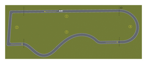
The driver starts the test from the starting point O, driving counterclockwise, and under the premise of ensuring safe vehicle control, accelerates with the maximum speed he can exert in a straight road section, then brakes, and turns into a short straight road section after coming to a complete stop at point A. This part simulates a straight line in the actual road, reflecting the driver’s degree of confidence in the acceleration and braking performance of the vehicle under different road conditions; then accelerate and brake again, and enter the right-angle curve section after completely stopping at point B, simulating the actual road 90° turn to reflect the driver’s trust level during the turning process after emergency braking; the driver then passes through S-turns and U-turns at top speed to simulate the long radius curves of lane change overtaking routes and ramps on real roads. Finally stop at the starting point O. If the driving process exceeds the test road, it is necessary to restart. This comprehensive procedure constitutes a full test cycle. In order to minimize the test error, each tester is required to perform the test process 4 times under the same driving scenario.
Data acquisition: We employed the VCDS diagnostic system as our data acquisition equipment. The parameters collected encompass vehicle speed, engine speed, engine torque, throttle opening, throttle opening change rate, brake pressure, brake pressure change rate, steering angle, steering angle speed, lateral acceleration, and other relevant metrics.
2.2. Driver Brake Operation Reaction Time Experiment
Since it is infeasible to measure a driver’s reaction time in a real-car test, we employ a driving simulator for this purpose, as shown in Figure 2.
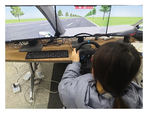
Experimental procedure: A virtual urban road environment was generated using UC-win/road. At intervals of 500 m, signs alerting the driver to execute an emergency brake were strategically positioned. Simultaneously, the word “Brake!!!” was displayed at the top center of the screen. The system recorded the driver’s reaction time when initiating emergency braking. Importantly, subjects were not provided advance notice of when the signs would appear during the test. Each subject was required to perform 10 trials in each driving scenario.
Data acquisition: Data collection is performed through UC-win/road. Record the time tz when each “Brake!!!” appears and the time tb when the brake signal appears. The interval between these times represents the driver’s reaction time for initiating a braking operation ti = tb − tz.
2.3. Experiment Data Preprocessing
Initially, the real vehicle test data undergoes pre-processing. The overall deceleration data from the four road sections is used to characterize the TLD. Since each road section impacts the driving trust level differently, and the maximum braking deceleration values vary significantly for each sample across different sections, hierarchical analysis is employed to assign appropriate weights to the four test sections, determining the weights for straight-line driving, right-angled curves, S-curves, and U-curves: ωn = (ω1, ω2, ω3, ω4) = (56.94%, 25.46%, 11.00%, 6.60%).
As a result, the results of the weighted maximum braking deceleration values for each tester at different tire–road coupling coefficients can be obtained, as shown in Table 1.
| Test subject number | Different tire–pavement coupling conditions | |||||||||
|---|---|---|---|---|---|---|---|---|---|---|
| μ1 | μ2 | μ3 | μ4 | μ5 | μ6 | μ7 | μ8 | μ9 | μ10 | |
| 1 | 5.999 | 5.235 | 5.055 | 4.977 | 4.289 | 4.120 | 4.062 | 3.420 | 2.755 | 2.164 |
| 2 | 4.552 | 3.722 | 3.625 | 3.502 | 3.255 | 3.102 | 2.746 | 1.122 | 1.001 | 0.624 |
| 3 | 4.422 | 3.624 | 3.452 | 3.122 | 3.025 | 3.022 | 2.618 | 1.002 | 0.790 | 0.565 |
| 4 | 4.103 | 3.201 | 3.125 | 2.855 | 2.598 | 2.265 | 2.023 | 0.984 | 0.752 | 0.512 |
| 5 | 2.775 | 1.749 | 1.666 | 1.210 | 1.002 | 0.756 | 0.554 | 0.433 | 0.226 | 0.195 |
| 6 | 2.602 | 1.525 | 1.525 | 1.138 | 1.001 | 0.763 | 0.720 | 0.600 | 0.531 | 0.122 |
| 7 | 4.621 | 3.826 | 3.531 | 3.502 | 3.012 | 3.001 | 2.525 | 1.489 | 1.162 | 0.525 |
| 8 | 4.619 | 3.601 | 3.505 | 3.201 | 3.132 | 2.828 | 2.612 | 1.057 | 0.998 | 0.602 |
| 9 | 5.312 | 5.042 | 4.731 | 4.521 | 4.487 | 4.099 | 4.012 | 3.120 | 2.625 | 1.923 |
| 10 | 2.621 | 1.606 | 1.465 | 1.009 | 0.848 | 0.423 | 0.201 | 0.196 | 0.169 | 0.156 |
Thus, the maximum acceleration weighted value for each test participant under different tire and road coupling coefficients can be obtained, as shown in Table 2.
| Test subject number | Different tire–pavement coupling conditions | |||||||||
|---|---|---|---|---|---|---|---|---|---|---|
| μ1 | μ2 | μ3 | μ4 | μ5 | μ6 | μ7 | μ8 | μ9 | μ10 | |
| 1 | 11.565 | 9.897 | 9.448 | 9.264 | 8.944 | 8.265 | 4.894 | 3.862 | 2.362 | 1.834 |
| 2 | 8.179 | 6.619 | 5.172 | 4.056 | 3.382 | 2.323 | 1.148 | 0.828 | 0.731 | 0.328 |
| 3 | 8.750 | 6.189 | 5.616 | 4.278 | 3.079 | 2.167 | 1.118 | 0.613 | 0.526 | 0.322 |
| 4 | 8.329 | 6.339 | 5.112 | 4.047 | 3.197 | 2.115 | 1.413 | 1.010 | 0.824 | 0.223 |
| 5 | 6.313 | 5.345 | 4.193 | 3.080 | 2.114 | 1.113 | 0.913 | 0.658 | 0.313 | 0.049 |
| 6 | 6.090 | 5.198 | 4.060 | 3.998 | 2.093 | 1.168 | 0.916 | 0.650 | 0.358 | 0.021 |
| 7 | 8.305 | 6.202 | 5.061 | 4.904 | 3.214 | 2.952 | 1.519 | 1.114 | 0.710 | 0.327 |
| 8 | 8.341 | 6.465 | 5.204 | 4.014 | 3.144 | 2.032 | 1.249 | 0.825 | 0.705 | 0.370 |
| 9 | 11.546 | 9.311 | 9.115 | 9.013 | 8.354 | 8.027 | 4.645 | 3.131 | 2.034 | 1.648 |
| 10 | 6.370 | 5.027 | 4.131 | 3.005 | 2.713 | 1.346 | 0.252 | 0.643 | 0.352 | 0.026 |
To preprocess the driver’s reaction time data, we calculated the average reaction time from 10 tests conducted for each subject under various road surface and tire conditions, as shown in Table 3.
| Test subject number | Different tire–pavement coupling conditions | |||||||||
|---|---|---|---|---|---|---|---|---|---|---|
| μ1 | μ2 | μ3 | μ4 | μ5 | μ6 | μ7 | μ8 | μ9 | μ10 | |
| 1 | 0.55 | 0.60 | 0.65 | 0.68 | 0.71 | 0.89 | 0.92 | 1.01 | 1.20 | 1.25 |
| 2 | 1.20 | 1.23 | 1.26 | 1.30 | 1.34 | 1.37 | 1.40 | 1.45 | 1.48 | 1.52 |
| 3 | 1.18 | 1.21 | 1.25 | 1.28 | 1.32 | 1.36 | 1.42 | 1.47 | 1.50 | 1.54 |
| 4 | 1.19 | 1.22 | 1.25 | 1.29 | 1.33 | 1.36 | 1.41 | 1.46 | 1.49 | 1.53 |
| 5 | 1.55 | 1.61 | 1.65 | 1.72 | 1.76 | 1.78 | 1.81 | 1.84 | 1.88 | 2.10 |
| 6 | 1.53 | 1.57 | 1.60 | 1.64 | 1.71 | 1.76 | 1.82 | 1.86 | 1.89 | 2.20 |
| 7 | 1.10 | 1.21 | 1.25 | 1.28 | 1.32 | 1.35 | 1.40 | 1.45 | 1.48 | 1.51 |
| 8 | 1.18 | 1.21 | 1.25 | 1.28 | 1.32 | 1.36 | 1.42 | 1.47 | 1.50 | 1.54 |
| 9 | 1.19 | 1.22 | 1.25 | 1.29 | 1.33 | 1.36 | 1.41 | 1.46 | 1.49 | 1.53 |
| 10 | 1.55 | 1.61 | 1.65 | 1.72 | 1.76 | 1.78 | 1.81 | 1.84 | 1.88 | 2.10 |
3. A Safe Distance Model Based on TLD
In the existing research on safe following distance models, the fixed safe distance model is simple to calculate, but its threshold is fixed and cannot adapt to dynamic changes in the preceding vehicle’s state or the environment. The safe distance model based on the braking process analyzes emergency braking distance through dynamics, but it assumes that vehicles brake at maximum deceleration, which does not align with actual driving behavior. The model based on time headway is only suitable for the following scenarios with relatively low relative speeds, failing to account for drivers’ subjective factors and environmental variables, thus limiting its applicability. The driver-estimated safe distance model incorporates drivers’ subjective perceptions and experiential parameters, but it suffers from an overemphasis on subjectivity, difficulty in measuring parameters, and lower model accuracy. The model based on the road surface adhesion coefficient considers road conditions but overlooks individual driver differences, such as the variation in vehicle performance exhibited by different drivers in the same emergency scenario. As a result, the model’s calculated outcomes deviate from the driver’s expected safe distance and driving habits.
In summary, this paper fully considers the shortcomings of existing models, integrates human, vehicle, and road-related factors and combines them with the second part of the article, in which a safe distance model based on TLD is developed in this section.
3.1. Development of a Safe Distance Model Based on TLD
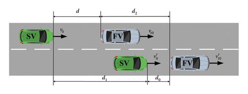
3.1.1. Safe Distance for the FV at Constant Speed
If the speed of the main vehicle (MV) is less than or equal to the speed of the FV vt0, v0 ≤ vt0, a collision between the two vehicles is avoided. However, if v0 > vt0, if the MV and the FV fail to maintain a reasonable distance, a collision may occur after a period of braking. Consequently, this operational scenario is exclusively examined concerning safe distances when v0 > vt0.
3.1.2. Safe Distance for the FV Under Decelerated Driving Conditions
The deceleration of the front car to slow down the driving deceleration is at1, and the initial braking speed is vt0; as the driver can play the braking deceleration is , the initial braking speed is v0.
At this point, the initial braking speed of the two cars exists in three cases: v0 > vt0, v0 = vt0, v0 < vt0. There are also three braking deceleration scenarios for both cars: , , . If the car slows down to the same speed as the vehicle in front, the car is out of danger.
3.1.2.1.
To make v > 0, take aivt0 ≥ at1v0. If v < 0, it means that the MV is out of danger only when it is braked to a stop.
When v0 < vt0, there is no danger of collision between the two vehicles.
3.1.2.2.
To make v > 0, take . If v < 0, it means that the MV is out of danger only when it is braked to a stop.
When v0 < vt0, , v < 0 there is no danger of collision.
3.1.2.3.
At this time, there are three cases of the initial braking speed of the two vehicles: v0 > vt0, v0 = vt0, v0 < vt0. In this scenario, the speeds of the two vehicles are equal only when both vehicles have reached a speed of 0.
There is no risk of collision when v0 < vt0.
When v0 = vt0, .
3.1.3. Safe Distance Under Accelerated Driving Conditions of the FV
The acceleration of the FV accelerating driving is at2; at this time, during braking of initial speed of the two cars, there are two situations: if v0 ≤ vt0, at this time, the two cars will not have collision danger; if v0 > vt0, at this time, there may be collision danger. When the MV decelerates to the same speed as the FV, it is out of danger.
3.2. Analysis of Experiment Data and Safe Distance Model
3.2.1. Estimation of Tire–Road Surface Coupling Coefficients
According to the real vehicle test data, select the data point of the maximum braking pressure with ABS intervention under each adhesion coefficient at which the braking deceleration is the maximum value. The value of the adhesion coefficient between the tire and the road surface can be calculated from equation (16). The calculation results are shown in Table 4.
| Road conditions | Tire conditions | μn value |
|---|---|---|
| Asphalt | Snow tire | μ1 0.86792 |
| Four-season tire | μ2 0.71828 | |
| Gravel | Snow tire | μ3 0.67664 |
| Four-season tire | μ4 0.62358 | |
| Wet | Snow tire | μ5 0.5399 |
| Four-season tire | μ6 0.51369 | |
| Snow | Snow tire | μ7 0.43625 |
| Four-season tire | μ8 0.40942 | |
| Ice | Snow tire | μ9 0.31776 |
| Four-season tire | μ10 0.24827 | |
3.2.2. Analysis of Brake Deceleration and Brake Application Reaction Time
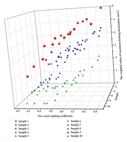
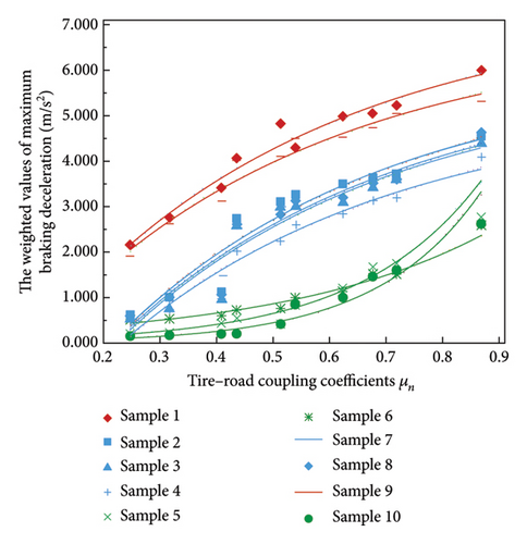
Utilizing data from both Tables 1 and 4, a comparative and analytical examination of the weighted values of maximum braking deceleration by the participants under various tire–road coupling coefficients μn was performed. The results of this comparison are presented in Figure 4.
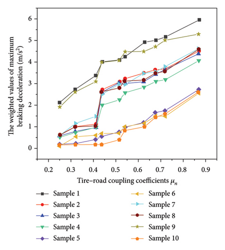
Figure 4 illustrates that, for the same sample, the weighted value of the maximum braking deceleration increases with an increase in μn. This suggests that improved road surface and tire conditions correspond to higher TLD and the ability to apply greater braking deceleration under extreme working conditions. These findings align with real-world observations. For different samples, under the same μn, the weighted values of maximum braking reduction speeds for samples 1 and 9 are relatively high, while samples 2, 3, 4, 7, and 8 exhibit intermediate values. In contrast, samples 5, 6, and 10 have lower weighted values. This observation indicates that under identical extreme working conditions, samples 1 and 9 demonstrate the highest TLD and the ability to apply greater brake reduction speeds. Samples 2, 3, 4, 7, and 8 closely follow, while samples 5, 6, and 10 exhibit the smallest values.
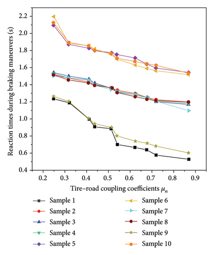
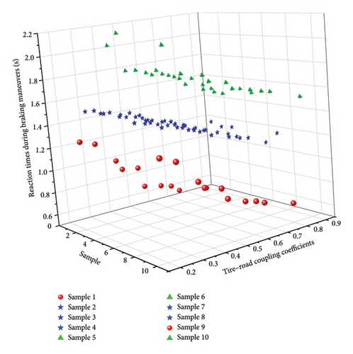
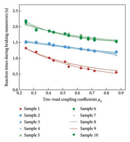
Using data from both Tables 3 and 4, a comparative analysis was conducted to compare the mean values of subjects’ reaction times during braking maneuvers under various tire–road coupling coefficients μn.
Figure 5 illustrates that, for the same sample, a smaller μn corresponds to longer driver reaction times during braking. This relationship can be attributed to the tense state of the driver’s nerves under poor road surface and tire conditions. In such circumstances, emergencies can induce panicky responses, and the driver’s inaccurate judgment of road surface conditions leads to extended reaction times. For different samples with the same μn, samples 1 and 9 exhibit relatively short reaction times, indicating the highest TLD. Following them, samples 2, 3, 4, 7, and 8 have intermediate reaction times, while samples 5, 6, and 10 demonstrate the longest reaction times. This observation aligns with the results of the analysis of weighted braking deceleration values.
3.2.3. Classification of TLD and Models for Braking Processes
In Figures 6 and 7, the trends of the maximum weighted brake deceleration values and the operating reaction times for all the samples are classified into three categories. Therefore, in this paper, the TLD (σ) is classified into three levels of high, medium, and low, represented by the letters “H,” “M,” and “L,” respectively. The greater the braking deceleration a driver can achieve in an emergency, the shorter the required reaction time, and the correspondingly higher the TLD. Subsequently, we analyze and discuss the data of the subjects falling within these three categories of TLD. The classification results, coupled with the coefficients between tires and road surfaces μn, are utilized to refine and ti in the established safe distance model, which is based on TLD. This refinement process also serves to further classify the model.
3.3. Validation and Application of a Safe Distance Model Based on TLD
3.3.1. Validation of the Safe Vehicle Distance Model
Due to the limitations of real vehicle test conditions, we adopted the UC/win-road driving simulator to create a simulated experiment environment for verification.
The simulation scenario is a two-vehicle follow-up scenario. In this scenario, the FV maintains a constant speed of 60 km/h. As per the analysis conducted in the previous section, it was determined that when the FV is traveling at a constant speed, the speed of the MV exceeding that of the FV may lead to a hazardous situation. Therefore, the speed of the MV was set at 70 km/h. For the validation test, we selected a driver from each of the three categories of TLD among the subjects. The validation tests were carried out under varying road surface conditions and adhesion coefficients ranging from μ1 ~ μ10. After the start of the experiment, the participants had a period of stable following time. When the brake lights of the lead vehicle turned on, the participants were required to initiate an emergency brake maneuver until the vehicle came to a complete stop. Subsequently, we calculated the safe distance for each driver under different road adhesion coefficients based on the data collected, as shown in Figure 10.
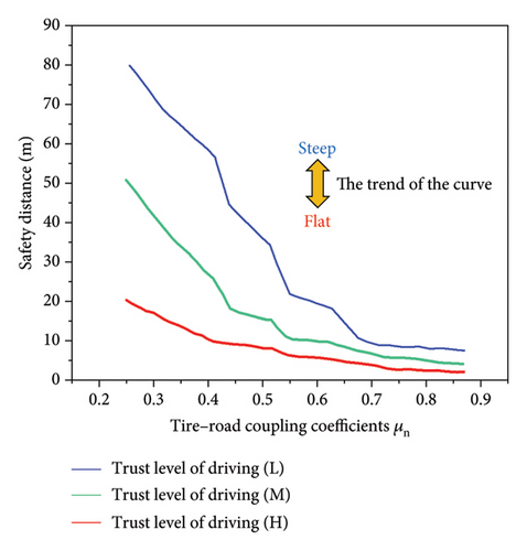
Figure 10 shows that the safe following distances for drivers with different TLD are different for different road adhesion conditions. For the same tire–road adhesion coefficient μn, the higher the TLD, the shorter the required safe following distance. This demonstrates that drivers with a high TLD have a clear understanding of vehicle and road conditions, react swiftly in emergencies, fully utilize the vehicle’s performance, and can execute an emergency stop within a short distance to avoid danger. Under different tire–road adhesion coefficient conditions, the higher the μn, the shorter the required safe following distance for the driver. Meanwhile, the trend of the σ = H curve is smoother, while the trend of the σ = L curve is more drastic, indicating that drivers with low TLD are strongly influenced by the road conditions and need to maintain a longer following distance under low μn. Through the above analysis, it has been verified that the safe following distance required by different drivers varies. Therefore, in the design of driver assistance warning systems, it is necessary to take into account the individual characteristics of drivers. Considering both traffic efficiency and driving safety, different safety warning thresholds should be assigned based on different TLD.
3.3.2. Application of the Safe Vehicle Distance Model
When the driver’s reaction time is measured, under the known road and tire conditions, the established database can be used to determine the braking deceleration that the driver can exert, thereby specifying the TLD and accordingly obtaining the appropriate safe following distance that should be maintained.
4. An Overtaking Model for Two-Way Dual Carriageways Based on TLD
Currently, both domestic and international studies have explored the safety of overtaking, with most research focusing on detailed analyses of vehicle overtaking behavior. However, few studies consider the impact of individual driver differences on overtaking behavior, resulting in models with insufficient accuracy. In fact, there are differences in each driver’s cognition of the critical distance that triggers the expectation of overtaking, which stems from their different levels of trust in their vehicles and current road conditions. When a driver operates a vehicle with strong acceleration performance under favorable road conditions, the critical following distance is smaller, and the safe distance required for overtaking also varies accordingly.
This paper builds on existing research as the foundation, takes vehicle operational characteristics as the benchmark, and considers individual driver differences. In conjunction with the second part of this paper, we have developed an overtaking model for two-way dual carriageways based on the TLD. The model is able to determine the minimum overtaking distance required for each driver to complete the entire overtaking maneuver and provide drivers with an early warning of whether it is safe to overtake on real roads. These results lay the foundation for ensuring the safety of the overtaking process on real roads.
4.1. Development of an Overtaking Model for Two-Way Dual Carriageways Based on TLD
4.1.1. Analysis of the Overtaking Process
4.1.2. Vehicle Key Point Definition
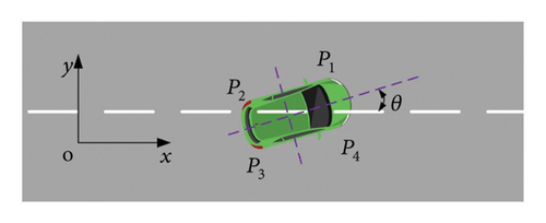
In this study, the dimensions of the vehicle are simplified for the sake of analysis. The vehicle is represented as a rectangle, as illustrated in Figure 13. Specifically, the four crucial points defining this rectangle are identified as follows: the left-front corner point, the left-rear corner point, the right-front corner point, and the right-rear corner point, denoted as Pi (i = 1, 2, 3, 4).
4.1.3. Analysis of Overtaking Safety Distances
4.1.3.1. Analysis of Safe Distances to the Point of First Impact
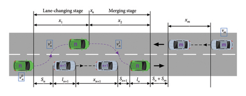
The overtaking vehicle “n” initiates the overtaking at time t = 0, with an adaptation time before overtaking denoted as ta. During the overtaking maneuver, the risk of a rear-end or side collision between the overtaking vehicle and the overtaken vehicle exists. In this overtaking scenario, where the overtaken vehicle maintains a constant speed, if the overtaking vehicle executes the maneuver with a certain lateral acceleration, it is highly likely that point P4 on vehicle “n” will collide with the overtaken vehicle. However, if no collision occurs at point P4, it implies that the two vehicles will not collide in the subsequent course of the maneuver. We define t2 as the time at which vehicle “n” reaches the collision point.
4.1.3.2. Analysis of Safe Distances to the Point of Second Collision Sn+1
4.1.3.3. Analysis of Safe Distances to the Point of Third Collision Sn + Sm
During the overtaking process, we do not account for the speed of the oncoming vehicle “m” being affected by the presence of overtaking vehicles. To guarantee an absolute absence of collision between overtaking vehicle “n” and oncoming vehicle “m”, the overtaking vehicle “n” must safely return to the original lane while maintaining a distance Sn + Sm from vehicle “m”. At this point, if no collision occurs, it ensures that during the merging process of vehicle “n” with vehicle “m”, no collision will transpire.
It is sufficient for Sn + Sm > 0, while the other variables maintain their previously defined meanings.
4.2. Analysis of Experiment Data and Overtaking Model
4.2.1. Comparative Analysis of Longitudinal Acceleration
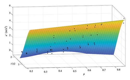
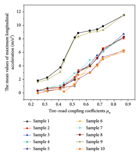
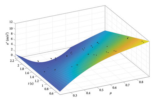
The mean values of maximum longitudinal acceleration for subjects at various tire–road coupling coefficients μn were compared and analyzed using data from Tables 2 and 4.
Figure 14 illustrates that, within the same sample, the mean acceleration increases with higher μn, implying that the better the road surface and tire conditions, the higher the driver’s driving trust and the greater the acceleration that can be exerted under extreme working conditions. Among different samples, samples 1 and 9 exhibit higher TLD at the same μn, while the others display lower TLD.
4.2.2. Classification of TLD and Models for Overtaking Processes
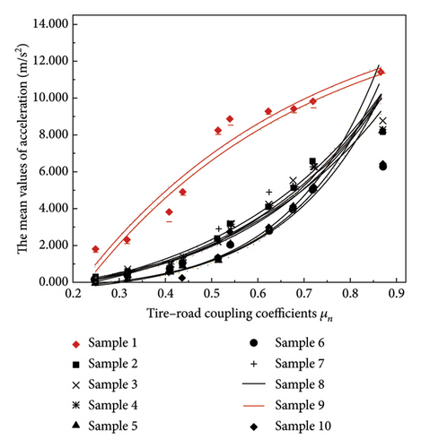
TLD is further divided into three degrees: samples 1 and 9 exhibit the highest TLD, σ = H. Samples 2, 3, 4, 7, and 8 are associated with a medium TLD, σ = M, while samples 5, 6, and 10 demonstrate a low TLD, σ = L. The mean longitudinal acceleration is closely tied to the tire–road surface coupling coefficient. Therefore, the ai in the established two-lane overtaking safety distance model based on TLD is refined by μn.
4.3. Validation and Application of Two-Way Dual Carriageways Overtaking Model Based on TLD
4.3.1. Verification of the Overtaking Model
Based on the analysis above, overtaking time correlates with three key variables: the speed of the overtaking vehicle vn, the speed of the overtaken vehicle vn+1, and the overtaking acceleration that the driver can apply during the overtaking maneuver. When vn+1 is significantly high, the overtaking time increases. Similarly, a higher shortens the acceleration time required, reducing the duration of the overtaking process. Consequently, drivers with greater TLD demand shorter overtaking times, aligning with real-world observations. The model will undergo validation via simulator testing, conducted in a two-way dual carriageway scenario.
In the first test, it was assumed that the initial speed of vehicle n + 1 was 60 km/h when overtaking, and maintained a constant speed. Vehicle n also had an initial speed of 60 km/h and performed overtaking at varying speeds. For each of the three driver types, one subject was chosen to participate in the overtaking test. Figure 16 demonstrates that, when confronted with identical overtaking scenarios, the overtaking time required by drivers with different TLDs is different. Drivers with high TLD can play a good acceleration performance during overtaking. According to safety distance analysis, they maintain a shorter safety distance before overtaking, resulting in the shortest overtaking time. Furthermore, it is observed that overtaking time diminishes as the speed of the overtaking vehicle increases, aligning with real-world observations.
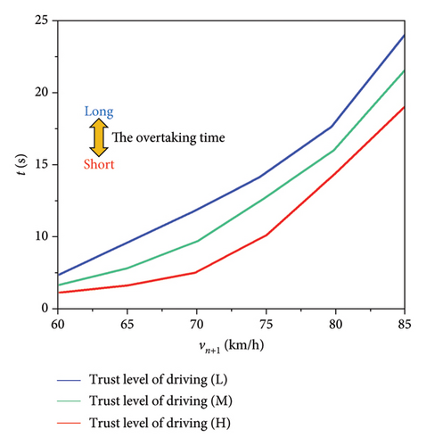
In the second test, we examined the impact of the overtaken vehicle’s speed on overtaking time. It was assumed that the overtaken vehicle was traveling at speeds of 60 km/h, 65 km/h, 70 km/h, 75 km/h, 80 km/h, and 85 km/h, while the overtaking vehicle maintained a constant speed of 100 km/h.
Figure 17 clearly demonstrates that as the speed of the overtaken vehicle increases, the overtaking time also lengthens. Furthermore, the impact of individual driver variations on overtaking time becomes more pronounced with higher vehicle speeds. Consequently, the influence of driver idiosyncrasies on the overtaking process becomes significant, particularly when overtaken vehicle speeds are high.
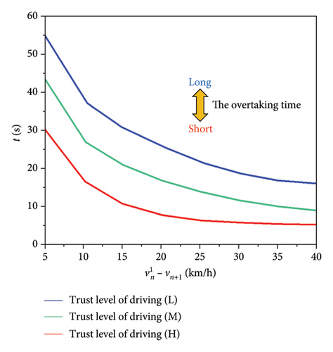
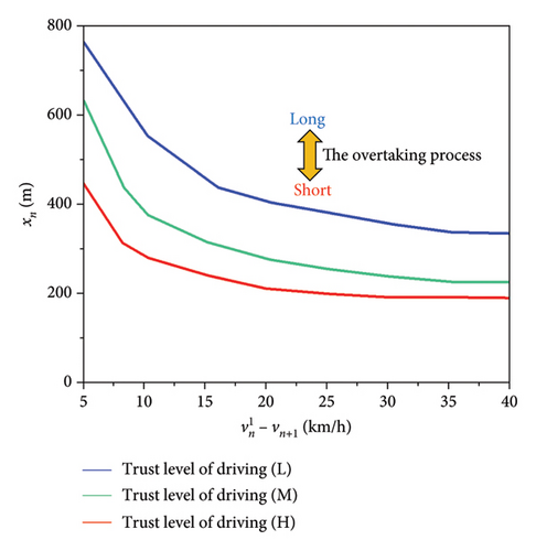
In the third test, both the overtaking vehicle and the vehicle being overtaken were initially set at a speed of 60 km/h. The vehicle being overtaken maintained a constant speed, allowing us to calculate the overtaking distances needed by various types of drivers when conducting overtaking maneuvers at different speeds.
Figure 18 reveals that a higher overtaking vehicle speed leads to a shorter overtaking process. In actual driving, drivers can appropriately increase the overtaking speed within the acceptable range to shorten the overtaking time and ensure safety. At the same time, the driver with high driving trust (σ = H) needs the smallest overtaking distance, followed by medium trust (σ = M), and low trust (σ = L) needs the largest distance, and with the increase of the speed difference between the two vehicles, the overtaking distance curve tends to be stable.
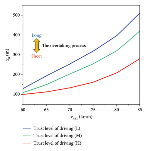
In the fourth test, the speed of the overtaken vehicle varied between 60 and 85 km/h. Figure 19 illustrates that as the speed of the overtaken vehicle increases, the overtaking distance also increases, resulting in a longer overtaking process. Additionally, as TLD decrease, the required overtaking distance increases, the impact of individual driver factors on overtaking distance increases as the speed of the overtaken vehicle rises.
In summary, the established overtaking model can match the overtaking distance and overtaking time of the actual overtaking process, and it effectively accounts for driver-specific factors, helping drivers complete the overtaking process safely and efficiently.
4.3.2. Application of the Overtaking Model
When the driver’s reaction time is measured in a way, under the known road and tire conditions, the established database can be used to determine the acceleration that the driver can exert, thereby specifying the TLD and accordingly obtaining the appropriate safe overtaking distance required for safe overtaking.
5. Conclusion
This paper focuses on analyzing the cognitive and behavioral characteristics of drivers during following and overtaking. Distinguishing from the cognitive hierarchy of the vehicle towards the driver, the concept of TLD is introduced from the perspective of the driver’s cognition of the car and the environment, and a safe distance model based on TLD and a two-way dual-lane overtaking model are proposed. These models aim to solve the problems of poor applicability and low group trust due to ignoring drivers’ individual differences and cognitive characteristics. Using data from real vehicle experiments and simulator tests, the models are optimized and refined to better align with individual drivers’ driving behaviors, significantly improving their accuracy and adaptability. A driving simulator was used to construct the corresponding scenarios to verify the validity of the model. Parameters such as safe following distance, overtaking time, and overtaking distance of drivers with different driving trust levels were obtained to verify the applicability of the model.
Therefore, in the design of the driver assistance warning system, individual driver characteristics can be fully considered, and different safety warning thresholds can be set according to different driving trust levels. In this way, the system can provide real-time alerts for drivers according to their safe driving and overtaking abilities during the driving process, thus ensuring the reliability and safety of vehicle traveling.
Ethics Statement
This study does not require ethical approval.
Consent
The authors have nothing to report.
Conflicts of Interest
The authors declare no conflicts of interest.
Author Contributions
The authors confirm contribution to the paper as follows: study conception and design: Wencai Sun, Xinze Liu; data collection: Shiwu Li, Xue Wen; analysis and interpretation of results: Xinze Liu, Xue Wen; draft manuscript preparation: Wencai Sun, Shiwu Li. All authors reviewed the results and approved the final version of the manuscript.
Funding
The project was supported by the General Program of the National Natural Science Foundation of China (Grant No. 52172385).
Open Research
Data Availability Statement
The data that support the findings of this study are available from the corresponding author upon reasonable request. In compliance with relevant laws, regulations, and research ethics, necessary data will be provided to qualified researchers.


