Fuel Consumption Prediction in Regional Transport Based on Selected Bus Line Characteristics
Abstract
From an operational, economic and environmental point of view, it is crucial for public transport authorities and operators to be able to estimate fuel consumption in suburban bus transport. This is especially important when planning a new bus line or re-routing an existing one. This paper aims to identify a simple model for predicting fuel consumption in suburban bus transport based on commonly available input data based on local conditions. The article deals with the issue of fuel consumption of a bus with a conventional compression ignition engine operating on suburban bus lines in a predetermined region in Slovakia. The selected indicators related to the operation of the studied bus are analysed, including the average speed of the bus, the average distance between stops, the road profile of the line and the ambient air temperature. The study was conducted using both long-term and short-term measurements, allowing for a comprehensive analysis of the data. Linear regression and polynomial regression were employed to determine the relationship between fuel consumption and the input data. The results of the long-term experimental measurements and regression analysis indicate that a second-degree polynomial regression is the most accurate method for predicting fuel consumption in suburban bus transport when considering the ambient air temperature. Short-term experimental measurements and regression analysis also demonstrate that a second-degree polynomial regression is the most effective approach for predicting fuel consumption in suburban bus transport, incorporating the average slope of the bus route and the average distance between bus stops. Average vehicle speed did not have a significant effect on predicting bus fuel consumption due to specific reasons that affect average velocity in very different ways.
1. Introduction
The impact of the transportation sector on energy demand and greenhouse gas production has increased over the past decades. Transportation is responsible for a significant portion of global energy demand, accounting for more than 20% of the total. In addition, the cost of energy represents a significant part of the total cost of urban and suburban bus transportation, accounting for more than 10%. In order to reduce fuel consumption, the optimal use of available resources constitutes a significant matter for each carrier [1]. The implementation of meticulous and comprehensive maintenance procedures, the installation of a variety of telematic and intelligent devices in vehicles and the improvement of the driving style of bus drivers are key methods for reducing fuel consumption costs [2].
The problem of fuel prediction for bus transit systems represents a significant research challenge for both academic and industrial communities. An accurate prediction model has the potential to facilitate numerous applications, including urban planning, emission reduction, anomaly detection and smart city development.
As the state of the art in this paper shows, many authors have tried to develop models that can calculate the predicted fuel consumption of buses based on selected input data. However, their common drawback is that they use complicated scientific methods that cannot be used by companies in common practice.
The aim of this paper is to develop an accessible model for the general practitioner to make fuel consumption predictions for suburban buses. For this reason, the input data chosen are those that are commonly available and known from vehicle operation and transport infrastructure characteristics. Regression analysis was used to investigate the dependence of fuel consumption on ambient air temperature, road profile of line, vehicle speed and distance between stops.
Although scientific methods based on neural networks are more accurate, they are difficult to apply in practice in transportation companies.
Therefore, the uniqueness of this work lies in the fact that, by using simple scientific methods, it provides an easy-to-use tool for practitioners (transport operators and public transport authorities) to predict fuel consumption in suburban bus transport based on commonly available input data characterising the operation of vehicles and transport infrastructure.
An important application of this model is the prediction of fuel consumption in suburban bus transportation, both in the context of modifications of existing bus lines and the design of new ones. The estimation of fuel consumption is essential for the calculation of operational parameters, economic costs and environmental impacts associated with changes in public transport.
1.1. State of the Art
Fuel consumption may be affected by various parameters such as vehicle speed, acceleration and braking, traffic conditions, vehicle technical characteristics, weather conditions and driving habits. These factors are often the subject of research aimed at the prediction of fuel consumption based on vehicle operating data.
Researchers have approached the estimation and prediction of fuel consumption using various techniques. Traditional methods include regression models, random forests, support vector machines and decision trees. Alongside them, neural network models such as BP neural networks, multiplayer perceptron networks and feedback neural networks are increasingly coming to the fore [3]. Each of these methods has its pros and cons. The performance of models is usually achieved through evaluation indicators, such as the coefficient of determination (R2), mean square error (MSE), root mean square error (RMSE), mean absolute percentage error (MAPE) or uncertainty with a 95% confidence level.
Regression analysis has been the most used traditional method. Newland [4] developed a regression function correlating bus fuel consumption with operational indicators such as vehicle speed, road profile grade, stop frequency, traffic volume and capacity and speed cycle changes. Ivković et al. [5] used the HDM model and regression analysis to analyse bus fuel consumption. The functional dependence between the speed of the diesel bus and its fuel consumption was found to be a second-order polynomial. Wang and Rakha [6] developed a convex second-order polynomial fuel consumption model for conventional diesel and hybrid-electric buses, with a special focus on driving characteristics. Regarding other traditional methods, Gong et al. [7] considered 21 factors causing fuel consumption to establish a random forest fuel consumption model. Zhang et al. [8] established a fuel consumption estimation model based on the least squares method using vehicle speed and acceleration. Zhu et al. [9] proposed a prediction model based on the improved decision tree. Hamed, Khafagy and Badry [10] proposed a machine learning model based on the support vector machine algorithm to predict vehicle fuel consumption.
In addition to traditional models, artificial neural network models and hybrid models have been used. Topić, Škugor and Deur [11] explored several models to predict fuel consumption based on vehicle speed, acceleration and road slope time series inputs using linear regression and neural networks. Ayman et al. [12] studied the impact of weather, temporal and spatial factors on diesel bus fuel consumption in Chattanooga, developing the FuelPred model using a recurrent neural network. Wysocki, Deka and Elizondo [13] applied polynomial regression and neural networks to model fuel consumption and reduce usage in heavy-duty vehicles. Recurrent neural network, nonlinear autoregressive model with exogenous inputs and generalised regression neural network were used for fuel consumption prediction in [14].
In several articles, authors have focussed on the parameters that most influence fuel consumption. Delgado, Clark and Thompson [15] developed and verified a mathematical-empirical methodology for predicting heavy-duty vehicle fuel consumption, identifying average velocity, average positive acceleration and the number of stops per distance as key model properties. Xiru, Zhu and Liping [16] proposed a statistical estimation model with categorical variables such as road type, time of day and week to predict fuel consumption. Ali and Piantanakulchai [17] investigated the effects of driving patterns on fuel consumption in heavy-duty vehicles, using variables such as distance travelled, instantaneous speed, hard braking, hard acceleration and engine idle timings, employing stepwise regression modelling. Zhang et al. [18] investigated fuel consumption for urban buses with various propulsion systems (e.g., natural gas, diesel and diesel/hybrid) on Beijing roads, highlighting the average speed as a key factor. Chen, Yeh and Wang [19] examined driving behaviour, vehicle characteristics, driver characteristics and weather in relation to fuel consumption. Frey et al. [20] investigated the impact of speed, acceleration and road grade on the fuel consumption of diesel and hydrogen fuel cell buses under real-world conditions. Ma et al. [21] used a gradient-boosting regression tree algorithm to rank influencing factors on energy consumption for diesel and electric uses in Beijing.
2. Methodology
Data collection was carried out using telematics systems. Two types of measurements were performed. A long-term measurement was done to determine the influence of the ambient temperature on the fuel consumption of the vehicle. In addition to the long-term measurement, two additional all-day measurements were made. These were necessary to determine the exact influence of the elevated bus line on vehicle fuel consumption. The measurements were carried out on existing lines in the Tatra region (the northeastern part of Slovakia), specifically in the districts of Poprad and Kežmarok, where the greatest distance was travelled, and then in the districts of Stará Ľubovňa, Levoča, Spišská Nová Ves and Sabinov.
These regions were suitable for this study because they had bus lines with different characteristics, varied terrain and diversified population distribution.
2.1. Long-Term Tracking of Vehicle Operating Data
Long-term monitoring of vehicle operational data was performed using telematics software for fleet management and monitoring the vehicle fleet (Figure 1). It works on the principle of collecting data from the vehicle’s control unit thanks to the appropriate hardware. These data are obtained from an on-board unit installed in the vehicle with a GPS antenna, which collects data on the vehicle’s behaviour in a contactless manner using a magnetic principle directly from the CAN bus and using the corresponding software which allows the storage, backup, processing and evaluation of the collected data from the vehicle control unit, the vehicle tachograph, the tachograph driver cards and vehicle location data from the on-board unit’s GPS antenna. Today, this software is based on shared online access via a web application. The analyses and resulting evaluations focus on the technological side of transportation, such as routing, navigation, evaluation of technical and economic data and monitoring of a number of other factors.

The latest trend in monitoring vehicle consumption through information telematics systems is the collection of data from the CAN bus or through the FMS gateway (output signal of data from the vehicle), i.e., reading data from the vehicle’s control unit [22]. Nowadays, this is the most commonly used method, which does not require any intervention in the fuel system, such as the installation of flow meters or level floats in the tank of the vehicle [23]. The output signal, which is further evaluated and processed by the software in relation to the work of the vehicle (km, mth), reaches the operator in the form of a numerical or visual output. It is a signal from the injectors when the system calculates the amount of fuel flowing based on the number and opening time of the injectors; the second way is to calculate the consumption according to the diagram of complete engine characteristics in relation to the current power and engine speed. The general principle of operation of the telematics system is depicted in Figure 1.
The long-term monitoring, collection and evaluation of selected operational data took place during the period from 20 October 2020 to 10 July 2021. There were approximately 235 measurement days with a total distance of almost 60,000 km. During the observed period, the vehicle always ran on a specific line with the same route and stopped with a specific number of transported passengers. The only difference during the monitored days could be the number of vehicle connections made, or in shunting and parking drives. However, these distances of exceptional differences were very small; therefore, their influence on the resulting evaluated data is negligible. The vehicle was also operated on different lines there in the monitored section. These were four specific days of operation that were excluded from the overall evaluation because their consideration could affect the resulting values.
2.2. Short-Term Tracking of Vehicle Operating Data
Short-term monitoring of the vehicle was carried out to allow more precise monitoring and evaluation of selected operating characteristics of the vehicle, which could not be obtained by long-term monitoring alone. This measurement was performed during two days of operation after 12 h operating cycles when the vehicle travelled a total distance of almost 700 km on both measurement days. During these measurements, it was observed how the average speed of the vehicle on the route, the road profile of the route, the average distance between stops or the stopping of the vehicle on the route affected the vehicle’s fuel consumption. It was necessary to use additional GPS devices to record the speed of the vehicle, its position and the immediate altitude at a frequency of 1 Hz. Such functionality was not provided by the telematics system used during the long-term monitoring.
2.3. Regression
In statistics, polynomial regression is a form of regression analysis in which the relationship between the independent variable X and the dependent variable Y is modelled as an nth degree polynomial in X. Polynomial regression fits a nonlinear relationship between the value of x and the corresponding conditional mean of y. Although polynomial regression fits a nonlinear model to the data, as a statistical estimation problem, it is linear because the regression function is linear in the unknown parameters estimated from the data. For this reason, polynomial regression is considered a special multiple linear regression case [24].
It is noteworthy that these models are all linear from the perspective of estimation, given that the regression function is linear with respect to the unknown parameters β0, β1, …, Consequently, the computational and inferential issues associated with polynomial regression can be fully resolved through the application of multiple regression techniques in least squares analysis. Therefore, for least squares analysis, the computational and inferential problems of polynomial regression can be completely addressed using the techniques of multiple regression. This is achieved by treating X, X2, … as being distinct independent variables in a multiple regression model [25].
For each variable included in the model, it is necessary to assess whether it is statistically significant or can be omitted from the model without affecting its quality. The significance of a given variable is evaluated through a significance test of the regression coefficient, conducted at the specified significance level α and assessed based on the p value of the test. If the p value is less than α, the coefficient is statistically significant, and the inclusion of the given explanatory variable in the model is justified. In the event that an explanatory variable’s coefficient is not statistically significant, it must be excluded from the model.
The quality of a regression model can be evaluated according to a number of criteria. First, the calculated p value for the full model is compared with the significance level α to determine whether the model is statistically significant (p value < α). The coefficient of determination, denoted as R2, expresses the proportion of the variability in consumption that can be explained by the model. The remaining proportion represents the unexplained variability.
In situations where two models appear to fit the data equally well, one must choose between them. In such cases, an F-test can be performed to ascertain which model is statistically better [26].
If the statistical significance of the regression model is confirmed, the model can be used to construct a prediction interval for a future value of yi of dependent variable Y. A prediction interval is defined as an estimate of an interval in which a future observation will fall, with a certain probability, given what has already been observed [27]:
3. Results
The data obtained from the experimental procedure were subjected to a comprehensive analysis, with the results divided into two categories: long-term and short-term measurements.
3.1. Long-Term Measurement Results
Due to the consistent nature of the vehicle’s operation, it was feasible to monitor and assess specific impacts on fuel consumption. Figures 2 and 3 provide an interpretation of some of the monitored operating data from the monitored period following individual measurement days.
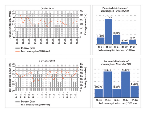
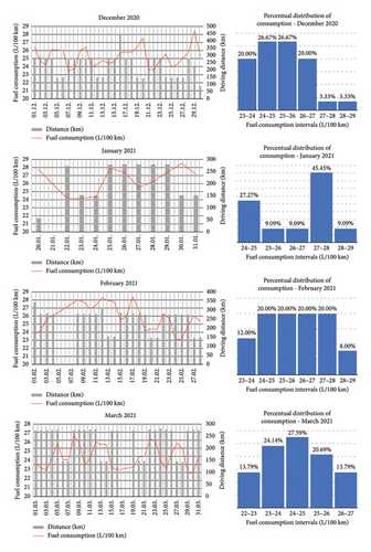
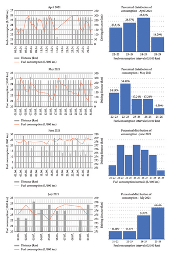
In the left part of the images, there are combined graphs representing the daily driving performance of the vehicle in km and the vehicle’s corresponding daily average fuel consumption in L/100 km.
In the right part of the images, the percentual distribution of the vehicle’s daily average fuel consumption is shown.
The monitored period was divided into four periods according to the seasons of the year. The autumn period was represented by October and November, the winter period was represented by December, January and February, the spring period by March, April and May and the summer period by June and July.
The overall numerical processing of the measured data is shown in Table 1 that is primarily divided into two parts. The left one represents the average and total monthly values of the selected monitored data (average fuel consumption, average air temperature, number of monitored days in operation and distance travelled by the vehicle). The right part statistically describes the minimums, maximums and median, as well as the standard deviation of average values of fuel consumption within individual months.
| Monitored period | Average consumption (L/100 km) | Average monthly temperature (°C) | Number of days in operation | Travelled distance (km) | Average fuel consumption (L/100 km) | |||
|---|---|---|---|---|---|---|---|---|
| Min | Max | Median | Standard deviation | |||||
| 10/2020 | 24.69 | 8.55 | 21 | 4591.44 | 23.06 | 27.09 | 24.81 | 1.03 |
| 11/2020 | 24.47 | 3.57 | 28 | 6648.78 | 22.57 | 26.99 | 24.55 | 1.30 |
| 12/2020 | 25.19 | 0.77 | 30 | 7008.79 | 23.43 | 28.44 | 25.24 | 1.21 |
| 01/2021 | 26.35 | −1.27 | 11 | 2322.46 | 24.10 | 28.51 | 27.14 | 1.55 |
| 02/2021 | 25.88 | 0.12 | 25 | 6250.51 | 23.06 | 28.37 | 25.99 | 1.59 |
| 03/2021 | 24.40 | 2 | 29 | 6958.13 | 22.56 | 26.76 | 24.37 | 1.26 |
| 04/2021 | 24.18 | 4.96 | 25 | 5717.45 | 22.30 | 26.09 | 24.13 | 1.27 |
| 05/2021 | 23.00 | 9.79 | 29 | 8181.37 | 21.07 | 25.35 | 22.79 | 1.20 |
| 06/2021 | 24.18 | 17.46 | 28 | 7748.91 | 21.22 | 27.13 | 24.16 | 1.56 |
| 07/2021 | 22.89 | 19.33 | 9 | 277.47 | 21.99 | 24.82 | 23.36 | 0.94 |
| Weighted average | 24.50 | 6.03 | ||||||
| Total numbers | 235 | 57,910.88 | 21.07 | 28.51 | ||||
The average value of fuel consumption of the vehicle over the entire monitored period was found to be 24.5 L/100 km. This is the average value, which is calculated based on the specific characteristics of the operation in question, including the number of passengers transported in the vehicle, the nature of the route on which the measurements were taken and the prevailing temperature conditions. The temperature conditions exerted a considerable influence on the fluctuations in fuel consumption in observed months. The average temperature for the entire observation period was 6.03°C, which is nearly identical to the yearly average temperature conditions for this region (two warmer months August and September were not included in the observation period). The average temperature for Poprad is around 9°C and for Stará Ľubovňa it is around 8°C. According to the aforementioned facts, it can be reasonably concluded that the results accurately reflect the year-round operational performance.
Two models were developed to express the dependence of the average consumption on the average daily temperature. The first is a linear model and the second is a quadratic model. The calculated p values indicated that both models were statistically significant. Based on the adjusted coefficients of determination, the quadratic model is better as it explains about 27% of the consumption variability compared to the linear model (15%). The remaining part of variability represents the unexplained variability attributed to unidentified factors, indicating that consumption is influenced by additional elements beyond temperature. Furthermore, the F-test was employed to compare the models. The F-statistic gave a value of 39.8939 compared to Fcrit = 3.88. This indicates that the quadratic regression model fits the data significantly better than the linear regression model.
The dependence of average fuel consumption on average daily air temperature is depicted in Figure 4.
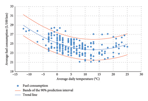
The calculated basic statistical indicators derived from the long-term experimental measurements are presented in Table 2. The calculated p value (Significance F in Table 2) for the full model is less than the significance level α (0.05), indicating that the model is statistically significant. The coefficient of determination 0.2764, denoted as R2, expresses the proportion of the variability (27.64%) in consumption that can be explained by the model, with the remaining proportion representing the unexplained variability. The significance of a given variable is evaluated through a significance test of the regression coefficient (p value in the table). Since all of them are less than the significance level α (0.05), the coefficients are statistically significant, justifying the inclusion of the given explanatory variables in the model.
| Summary output | |||||
|---|---|---|---|---|---|
| Regression statistics | |||||
| Multiple R | 0.5258 | ||||
| R square | 0.2764 | ||||
| Adjusted R square | 0.2702 | ||||
| Standard error | 1.3562 | ||||
| Observations | 234 | ||||
| ANOVA | |||||
| df | SS | MS | F | Significance F | |
| Regression | 2 | 162.3191 | 81.1596 | 44.1226 | 5.9E − 17 |
| Residual | 231 | 424.9034 | 1.83941 | ||
| Total | 233 | 587.2225 | |||
| Coefficients | Standard error | t stat | p value | ||
| Intercept | 25.1718 | 0.1171 | 215.0005 | 4.7E − 268 | |
| Temperature | −0.2204 | 0.0245 | −8.9789 | 9.81E − 17 | |
| Temperature2 | 0.0084 | 0.0013 | 6.3162 | 1.36E − 09 | |
- 2It is the calculation of objective statistical indicators to assess the relevance of the dependence of the measured variables.
3.2. Short-Term Measurement Results
The measurements were conducted along 12 lines in both directions within the specified region. The dataset recorded from short-term measurements represents comprehensive data divided into 25 section units, representing lines or parts of lines. These were selected based on their technical indicators to ensure the monitored characteristics exhibited minimal variation, thereby facilitating a more precise assessment of their influence on vehicle fuel consumption. For example, if there was a big change along the line, either in the distances between stops or in the slope ratios of the longitudinal line, it would be divided into sections, considering the most analogous conditions within them.
To ascertain the influence of selected characteristics of the transport infrastructure and operation on fuel consumption without the confounding effect of internal factors, all short-term measurements were conducted with the same vehicle, same driver and same number of passengers.
A summary of the measured values from the short-term experimental measurements is provided in Table 3.
| Track | Distance (km) | Average speed (km/h) | Road profile of the route | Average distance between stops (km) | Average consumption (L/100 km) | ||
|---|---|---|---|---|---|---|---|
| Total climb (m) | Total decline (m) | Average slope | |||||
| Sp. Štvrtok-SNV | 14.07 | 34.42 | 90 | −184 | −0.89% | 1.759 | 17.77 |
| PP-Sp. Štvrtok-KK | 34.62 | 34.21 | 567 | −619 | −0.15% | 1.282 | 24.55 |
| KK-Sp. Belá | 6.68 | 34.42 | 109 | −90 | 0.28% | 1.670 | 22.46 |
| Sp. Belá-Podolínec | 9.25 | 37.5 | 147 | −218 | −0.66% | 1.542 | 21.62 |
| Ľubotín-Lipany | 22.7 | 43.08 | 199 | −313 | −0.75% | 2.838 | 19.82 |
| Ľubotín-SL | 19.64 | 49.13 | 338 | −308 | 0.15% | 2.455 | 25.46 |
| SL-SSV | 35.9 | 40.51 | 518 | −542 | −0.07% | 1.561 | 25.07 |
| Hromoš-SL | 14.45 | 38.38 | 285 | −281 | 0.03% | 1.204 | 31.14 |
- Note: KK, Kežmarok; PP, Poprad.
- Abbreviations: SL, Stará Ľubovňa SNV, Spišská Nová Ves; SSV, Spišská Stará Ves.
The dependence of the average fuel consumption on the average vehicle velocity (i.e. technical, driving speed) on the examined bus line is shown in Figure 5.
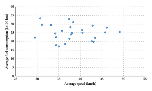
To ascertain the relationship between consumption and average speed, a regression model was constructed. Subsequently, p values were calculated in order to assess the statistical significance of this relationship. The p values for the linear model, the second-degree polynomial and the third-degree polynomial were 0.7722, 0.7614 and 0.8956, respectively. The p values are all greater than 0.05, indicating that the null hypothesis cannot be rejected at the 0.05 level of significance regarding the statistical insignificance of the regression model. Consequently, neither model is suitable for describing the given dependence. Furthermore, the regression coefficients are also statistically insignificant.
It can be concluded that, although fuel consumption is dependent on instantaneous speed, it is not possible to establish a meaningful correlation based on the average speed indicator alone. This is because the value of the average speed of the vehicle alone is not sufficiently reliable. The same nominal value of the average speed can be achieved if the vehicle moves through the entire monitored section at a constant speed, but also if it changes its instantaneous speed on this section with different driving dynamics, or stops, for example, at bus stops. Therefore, it is more important to monitor the dependence of fuel consumption on the number of stops, or on the distances between them.
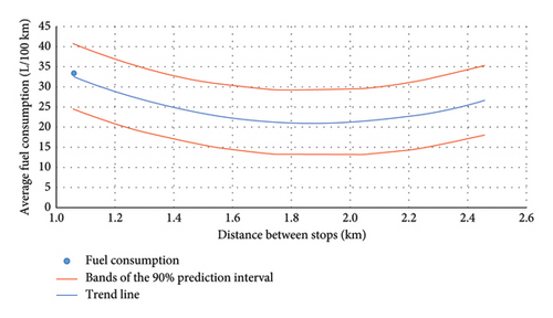
Initially, a linear regression model of the dependence of average consumption on the average distance between stops was created. The correlation coefficient was −0.487, the p value was 0.0319 and the coefficient of determination was 19%. Subsequently, a quadratic regression model was calculated with a p value of 0.0014 for the explanatory variable (the distance between stops on the route). Based on the coefficient of determination, the quadratic regression model explains about 46% of the variability of consumption. So, the distance between stops on the route significantly affects the average fuel consumption.
The dependence of the average fuel consumption on the average distance between stops on the examined bus line is depicted in Figure 6.
The calculated basic statistical indicators from short-term experimental measurements that monitor the dependence of fuel consumption on the average distance between stops are summarised in Table 4.
| Regression statistics | |||||
|---|---|---|---|---|---|
| Multiple R | 0.6815 | ||||
| R square | 0.4644 | ||||
| Adjusted R square | 0.4134 | ||||
| Standard error | 3.4522 | ||||
| Observations | 24 | ||||
| ANOVA | |||||
| df | SS | MS | F | Significance F | |
| Regression | 2 | 217.0012 | 108.500 | 9.1042 | 0.0014 |
| Residual | 21 | 250.2717 | 11.9177 | ||
| Total | 23 | 467.2729 | |||
| Coefficients | Standard error | t stat | p value | ||
| Intercept | 81.1601 | 15.0411 | 5.3959 | 2.37E − 05 | |
| Distance between stops | −64.0389 | 18.1875 | −3.5210 | 0.0020 | |
| Distance between stops2 | 17.0187 | 5.21281 | 3.2648 | 0.0037 | |
- 2It is the calculation of objective statistical indicators to assess the relevance of the dependence of the measured variables.
The area with the shortest distances between stops, as illustrated in Figure 6, is also the area with the lowest average vehicle speed on the route. This area represents the highest fuel consumption in the graph. This is due to the fact that the vehicle frequently stops and starts, which has a negative effect on immediate fuel consumption. The curve subsequently declines. This indicates that the vehicle’s fuel consumption decreases as the distance between stops increases because the vehicle’s driving is smoother, and the fuel consumption then decreases. However, from a certain point, the vehicle’s fuel consumption on the route increases again along with the increasing distance between the vehicle’s stops. This is because the vehicle slows down and accelerates less, i.e., the inertial resistance is not so significant, and currently the vehicle reaches higher speeds on longer sections between stops. This fact causes an increase in the energy demand due to higher driving resistances acting at higher driving speeds. This ultimately causes a higher rate of fuel consumption.
In this particular case, the optimal average distance between stops, which would result in the lowest average fuel consumption, would be 1.88 km.
The average measured values of vehicle deceleration were 1.3 m/s2 in the whole velocity range (from 80 km/h to 0 km/h). The acceleration values were approximately 1.2 m/s2 from 0 to 50 km/h and 1.1 m/s2 from 50 to 80 km/h velocity. These values represent the usual vehicle operation on the bus line.
The interval marked by the red curves on the graph in Figure 6 can be utilised by the carrier during real operation to check fuel consumption, for example, whether there is illegal theft of fuel, its loss or whether the driver’s bad driving technique or a hidden technical fault on the vehicle does not cause excess fuel consumption.
A linear regression model was constructed to examine the relationship between average consumption and average slope along the specified examined bus line. The correlation coefficient was 0.7976, the p value was 1.8·10−6 and the coefficient of determination was about 64%.
Figure 7 shows the course of dependence of the average fuel consumption on the average slope of the line route.
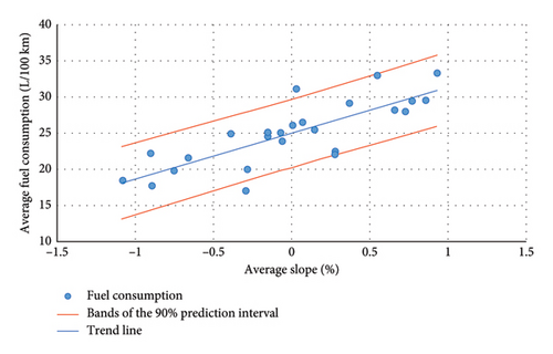
The calculated correlation between the average fuel consumption and the increasing average slope of the route is consistent with physical dependence. The instantaneous fuel consumption of the vehicle is directly proportional to the resistance resulting from the slope of the line route.
The calculated basic statistical indicators from short-term experimental measurements that monitor the dependence of fuel consumption on the average slope of the line route are presented in Table 5.
| Regression statistics | |||||
|---|---|---|---|---|---|
| Multiple R | 0.7976 | ||||
| R square | 0.6362 | ||||
| Adjusted R square | 0.6204 | ||||
| Standard error | 2.7993 | ||||
| Observations | 25 | ||||
| ANOVA | |||||
| df | SS | MS | F | Significance F | |
| Regression | 1 | 315.1647 | 315.1647 | 40.2193 | 1.8E − 06 |
| Residual | 23 | 180.2315 | 7.8362 | ||
| Total | 24 | 495.3962 | |||
| Coefficients | Standard error | t stat | p value | ||
| Intercept | 25.0110 | 0.5599 | 44.6733 | 7.42E − 24 | |
| Average slope | 6.3061 | 0.9944 | 6.3419 | 1.8E − 06 | |
A regression model depending on the average speed, the average distance between stops and the average slope of the route was created. The calculated p value indicated that the regression model is statistically significant at the 0.05 level. However, the regression coefficient for the average speed was found to be statistically insignificant (p value is 0.09 > 0.05), and thus it was excluded from the model.
| Regression statistics | |||||
|---|---|---|---|---|---|
| Multiple R | 0.8479 | ||||
| R square | 0.7190 | ||||
| Adjusted R square | 0.6935 | ||||
| Standard error | 2.5154 | ||||
| Observations | 25 | ||||
| ANOVA | |||||
| df | SS | MS | F | Significance F | |
| Regression | 2 | 356.1973 | 178.0987 | 28.148 | 8.62E − 07 |
| Residual | 22 | 139.1989 | 6.3272 | ||
| Total | 24 | 495.3962 | |||
| Coefficients | Standard error | t stat | p value | ||
| Intercept | 29.7017 | 1.9094 | 15.5552 | 2.36E − 13 | |
| Average slope | 5.6870 | 0.9260 | 6.1414 | 3.51E − 06 | |
| Distance between stops | −2.9041 | 1.1404 | −2.5466 | 0.018391 | |
The regression coefficient 5.69 can be interpreted as follows: for each 1% increase in the slope, there is a corresponding 5.69 L/100 km increase in the average fuel consumption at an unchanged distance between stops.
The regression coefficient −2.90 indicates that an increase in the distance between stops of 1 km results in a reduction in the fuel consumption of 2.90 L/100 km, with no change in the resulting average slope of the route.
| Regression statistics | |||||
|---|---|---|---|---|---|
| Multiple R | 0.8819 | ||||
| R square | 0.7777 | ||||
| Adjusted R square | 0.7460 | ||||
| Standard error | 2.2898 | ||||
| Observations | 25 | ||||
| ANOVA | |||||
| df | SS | MS | F | Significance F | |
| Regression | 3 | 385.2915 | 128.4305 | 24.4952 | 4.69E − 07 |
| Residual | 21 | 110.1047 | 5.2431 | ||
| Total | 24 | 495.3962 | |||
| Coefficients | Standard error | t stat | p value | ||
| Intercept | 45.9604 | 7.1175 | 6.4574 | 2.12E − 06 | |
| Average slope | 5.4038 | 0.8515 | 6.3464 | 2.72E − 06 | |
| Distance between stops | −21.809 | 8.0922 | −2.6951 | 0.0136 | |
| Distance between stops2 | 5.0663 | 2.1507 | 2.3556 | 0.0283 | |
- 2It is the calculation of objective statistical indicators to assess the relevance of the dependence of the measured variables.
The created quadratic regression model for the average consumption can be only used in monitored intervals for the resulting average slope of the route si ∈ [−1%; 1%] and the average distance between stops on the route vi ∈ [1 km; 2.5 km].
We can easily compare the linear and quadratic regression models based on the adjusted value of the coefficient of determination; the higher the value, the better the model. The linear model had a value of 0.6935, while the quadratic model had a value of 0.7460. Additionally, the F-test was employed to compare the models. The F-statistic yielded a value of 5.5491 in comparison to Fcrit = 4.32. This indicates that quadratic regression model fits the data significantly better than the linear regression model.
4. Discussion
Several authors have addressed the problem of increasing the efficiency of bus operations. Wang and Rakha [6] proposed a convex fuel consumption model for diesel and hybrid-electric buses with a focus on driving characteristics. Their findings revealed that buses cruising at speeds between 39 and 47 km/h within grades of 0%–8% had the lowest rate of fuel consumption. This model considers just the elevation of the road and the average speed, but without considering the distances between stops. However, the results of our study prove that not only the numerical value of the average speed but also the frequency of stops that affect it are decisive for the prediction of fuel consumption.
A similar statement can be applied to the model of Ivković et al. [5] who used quadratic regression models to determine the functional dependence between the speed of diesel buses and their fuel consumption according to the type of terrain (slope, average horizontal curvature, average altitude and speed limit) by incorporating corrective factors of fuel consumption between design speed and operating speed.
The prediction of fuel consumption, which also considered driving dynamics, was dealt with by Ali and Piantanakulchai [17]. They used telematics data to analyse and predict fuel consumption of heavy-duty vehicles by stepwise regression. As explanatory variables were taken the travelled distance, instantaneous speed, number of hard braking per 100 km, number of hard accelerating per 100 km and engine idle time in one time fuel-filling. The R2 value was between 0.8573 and 0.9389. However, due to the different nature of the operation of a suburban bus compared to a heavy-duty vehicle, the results of this model are unsuitable for our use in public passenger transport. These vehicles are equipped with similar, sometimes the same engines, but their driving resistances, shape, size and mass are significantly different.
Another model that deals with the issue of neural networks is Topić, Škugor and Deur [11]. They employed a regression model and neural network model accounting for fuel consumption of buses based on vehicle velocity, acceleration and road slope time series inputs. The models exhibited an R2 value exceeding 0.9, indicating a high degree of accuracy. Nevertheless, in machine learning, overfitting may occur, which can negate the purpose of the machine learning model. Consequently, the high value of R2 cannot generalise effectively to new data.
In the article, we discussed the dependence of the average fuel consumption on the average distance between stops on the line which is only applicable to distances between stops from 1 km to 2.5 km. In this particular case, the optimal average distance between stops, which would result in the lowest average fuel consumption, would be 1.88 km. There are other points of view on the optimisation of distances between bus stops. Jin et al. [28] optimised a stop configuration based on total travel time. Wu, Jin and Yang [29] analysed transit stop spacing by the influence of general conditions such as household density, household income, trip distance and specific conditions such as traveller age, wait time, and trip frequency. Jin, Yu and Yang [30] analysed and modelled the effect of intermittent lane blockage at a curb-side bus stop on mixed traffic dynamics.
Our decision to use regression analysis for fuel consumption modelling was based on its advantages. Regression models are generally easier to understand and interpret. The results are often straightforward, allowing for better comprehension of the relationships between variables. Implementing and calculating regression models typically requires less time and computational resources than more advanced methods like neural networks or machine learning, which are unsuitable for use in the common practice of bus operators. Despite these advantages, more complex methods might be necessary in situations where the relationships between variables are complex or when dealing with large datasets that require advanced techniques for processing and analysis which was not our case.
The proposed model offers a straightforward method for estimating fuel consumption, which is widely applicable in practical settings. It fulfils a gap between the already published studies of this issue because it considers also vehicle dynamics by using simple scientific methods. Based on this model, the fuel consumption of a specific vehicle (in this case Iveco Crossway 10 E6) can be determined on a route with defined parameters. The model is most suitable for determining the energy requirements of selected road sections in practice for carriers while planning new bus lines that have not yet been operated as a basis for calculating the fuel consumption and the cost of operating a vehicle under normal operating conditions. Furthermore, the model can be employed in the event of a proposed alteration to the route of an existing bus line. Consequently, it is primarily utilised by bus operators and public transportation authorities.
It is important to consider fuel consumption not only in terms of its impact on operating costs but also in terms of its broader environmental implications. The proposed model can be utilised to evaluate the environmental impact of public transportation in terms of energy consumption and emissions.
This manuscript is focussed on the issue of fuel consumption of the bus with a compression ignition engine operated on lines of suburban transport in a particular territory. Predetermined attributes regarding the examined bus, such as the average bus speed, the average distance between stops, the road profile of the line and the ambient air temperature, were evaluated during the research. While investigating, for this purpose, an on-board unit was installed in the examined vehicle that collected data from a vehicle control unit as well as an external satellite antenna. The investigation itself was executed in two scenarios, both a long-term examination for nine months with a vehicle’s driving performance of 60,000 km and two short-term investigations over two days at a distance of 700 km to specify the data recorded. Subsequently, the impact of each finding on the fuel consumption of the examined vehicle was evaluated, and their statistical significance was determined.
Real fuel consumption depends not only on the technical characteristics of the vehicle, the transport infrastructure and the number and location of stops but also on the smoothness of the transport flow and the driving style of the bus driver. The technical characteristics of the vehicle and the transport infrastructure, as well as the number and location of stops, can be considered as unchanging characteristics over a period of time. Therefore, our model is based on these input data, which can be considered as constant. The current traffic flow and the driver’s driving style are indicators that could be changed over time. It is for this reason that our model does not incorporate these variables as input data; however, their influence is acknowledged in the graphs (Figures 4, 6, and 7) by the interval reserved by the red lines corresponding to the predictive bands of 90% of the data. This interval can be used by the carrier or the public transport authority to check the reality of fuel consumption, i.e., whether there is an illegal loss of fuel or a technical problem with the vehicle that increases fuel consumption above the average.
One of the limitations of the research lies in the defined characteristics, namely, the average bus speed, the average distance between stops, the road profile of the line and the ambient air temperature. Only these specific factors could have been monitored, examined and thereafter evaluated using the equipment at the authors’ disposal. A further limitation consists of a confined transport territory which was chosen to carry out all the measurements and investigations as well as a limited time period earmarked for the research by the supervisor of the study.
Partially different results may be obtained with other types of combustion engines with different power or with different bus designs. However, by applying the methodology used in this research, it is possible to obtain relevant results that are also valid for other types of buses or combustion engines.
The model may be partly employed in some related research and scientific pursuits. With regard to future research in this particular field, it is possible that the authors of the manuscript and other scholars may examine a broader range of technical parameters related to suburban bus transportation, beyond those considered in this study. Moreover, apart from the statistical considerations, the emphasis should also be placed on the economic evaluation of individual aspects of the conducted research. A detailed examination of the influence of the bus operation–defined indicators on fuel consumption, particularly in relation to the calculation of pertinent economic variables such as total transportation costs, return on investment, time, financial demand for investments in telematics equipment, profitability and other factors, would be advantageous.
5. Conclusion
In order to be sustainable in the long term, the transport system must be of sufficient quality from the passenger’s point of view and at the same time sufficiently efficient from the operator’s or public transport authority’s point of view. The efficiency of public passenger transport has a direct impact on operations and the economy, as well as on the environment. These aspects have to be considered when planning new suburban bus lines but also when modifying the existing bus routes.
This study presents a novel prediction model for estimating the fuel consumption of suburban buses. That means the study deals with the issue of environmental and energy efficiency of bus operations from the operator’s or public transport authority’s point of view. In order to predict the fuel consumption for a specific vehicle, it is necessary to consider a number of factors, including the external temperature, the average slope of the bus route and the distances between stops. These are indicators that are easy to identify and quantify. The advantage of this model is that it also takes into account the distance between stops, which has a direct impact on driving dynamics and the average speed of the vehicle.
- 1.
The relationship between the bus fuel consumption and the average daily temperature can be described by a quadratic function.
- 2.
Although bus fuel consumption is influenced by the average speed of the vehicle, these available data are insufficient for developing a reliable model for predicting fuel consumption.
- 3.
The distance between bus stops has a significant impact on fuel consumption (this fact influences also the average speed of the vehicle).
- 4.
The relationship between the bus fuel consumption and the distance between stops can be described by a quadratic function.
- 5.
The relationship between the bus fuel consumption and the average slope can be described by a linear function.
- 6.
The dependence of the bus fuel consumption on the average slope of the line route and the average distance between stops can be described by a polynomial function of the second degree (quadratic).
The efficiency of public passenger transport has a direct impact on operational effectiveness, economic activity and environmental sustainability. These factors must be taken into account when developing new suburban bus routes and modifying the existing bus routes. The presented model may be useful for such prediction, for example, by operators or public transport authorities.
Conflicts of Interest
The authors declare no conflicts of interest.
Funding
This work was supported by the National Science Fund of the Ministry of Education and Science of Bulgaria (project no. KP-06-H77/11 of 14.12.2023 “Modeling and development of a complex system for environmental and energy efficiency of urban transport”).
Open Research
Data Availability Statement
The data that support the findings of this study are available from the corresponding author, Martin Kendra, upon reasonable request.


