Volume 2025, Issue 1 5518224

Research Article

Open Access

A Simple and Effective Second-Order Numerical Algorithm for Tempered Fractional Differential Equation With Time Caputo-Tempered Fractional Derivative

Dechao Gao,

Dechao Gao

Department of Basic Education , Xinjiang University of Political Science and Law , Tumushuke , China

Search for more papers by this author

Zeshan Qiu,

Corresponding Author

Zeshan Qiu

[email protected]

orcid.org/0009-0009-2051-4651

Department of Basic Education , Xinjiang University of Political Science and Law , Tumushuke , China

Search for more papers by this author

Lizan Wang,

Lizan Wang

Department of Basic Education , Xinjiang University of Political Science and Law , Tumushuke , China

Search for more papers by this author

Jianxin Li,

Jianxin Li

Department of Basic Education , Xinjiang University of Political Science and Law , Tumushuke , China

Search for more papers by this author

Dechao Gao,

Dechao Gao

Department of Basic Education , Xinjiang University of Political Science and Law , Tumushuke , China

Search for more papers by this author

Zeshan Qiu,

Corresponding Author

Zeshan Qiu

[email protected]

orcid.org/0009-0009-2051-4651

Department of Basic Education , Xinjiang University of Political Science and Law , Tumushuke , China

Search for more papers by this author

Lizan Wang,

Lizan Wang

Department of Basic Education , Xinjiang University of Political Science and Law , Tumushuke , China

Search for more papers by this author

Jianxin Li,

Jianxin Li

Department of Basic Education , Xinjiang University of Political Science and Law , Tumushuke , China

Search for more papers by this author

First published: 23 May 2025

https://doi.org/10.1155/admp/5518224

Academic Editor: Shikha Binwal

Share a link

Email
Wechat
Bluesky

Abstract

This paper presents an efficient numerical scheme for the space–time tempered fractional convection–diffusion equation, where the time derivative is the Caputo-tempered fractional derivative and the space derivatives are the normalized left and right Riemann–Liouville tempered fractional derivatives. The time Caputo-tempered fractional derivative is transformed into time Riemann–Liouville tempered fractional derivative by the relationship between Caputo fractional derivative and Riemann–Liouville fractional derivative. Using the tempered weighted and shifted Grünwald difference operators to approximate the time-tempered fractional derivative and the space-tempered fractional convection–diffusion term, it is obtained that the time and space directions are both second-order precision. The stability and convergence of the proposed numerical scheme are analyzed by using the energy method with a little different from the existing work. It is found that the proposed scheme is unconditionally stable and convergent with order O(τ² + h²). Finally, some numerical examples are given to verify the effectiveness of the proposed scheme.

1. Introduction

In this paper, the following space–time tempered fractional convection–diffusion equation is considered:

(1)

where 0 < α, β < 1, 1 < γ < 2, λ₁, λ₂, λ₃ ≥ 0, and parameters l_β, r_β, l_γ, and r_γ are nonnegative constants, which satisfy that l_ξ + r_ξ ≠ 0(ξ ∈ {β, γ}), φ_l(t) ≡ 0 if l_ξ ≠ 0 and φ_r(t) ≡ 0 if r_ξ ≠ 0.

and

represent the normalized left and right Riemann–Liouville tempered fractional derivatives, respectively, which are defined as follows [1–3]:

(2)

(3)

Let n = ⌈ξ⌉, where

and

represent the left and right Riemann–Liouville tempered fractional derivatives, respectively, which are defined by the following:

(4)

The Γ(⋅) in here is the gamma function.

denotes the left Caputo-tempered fractional derivative, which is defined as follows:

(5)

According to the relationship between Caputo fractional derivative and Riemann–Liouville fractional derivative [4], we can deduce the following by simple calculation:

(6)

Substituting Equation (6) into Problem (1), then Problem (1) can be equivalently transformed and rewritten as follows:

(7)

Fractional derivative has been proposed for a long time. Due to the lack of understanding of its application in the real world, it is gradually known and studied by many scholars in the last half century. Fractional differential equations derived from fractional derivatives are widely used in many fields, such as groundwater hydrology, finance, plasma physics, and biology [5–12]. Because of the nonlocality of fractional derivatives, the analytical solutions of fractional differential equations are difficult to obtain, so it is urgent to develop numerical methods for solving fractional differential equations. Many scholars have done a lot of important work on fractional differential models and their numerical solutions [13–23].

Fractional differential equations include time-fractional differential equations, space fractional differential equations, and space–time fractional differential equations. Caputo fractional derivative generally describes time-fractional derivative, and Riemann–Liouville fractional derivatives generally describe space fractional derivatives. For Caputo fractional derivative, the idea of piecewise interpolation is generally used to approximate it, and L1 [24, 25], L1 − 2 [26], and L1 − 2_σ [27] formulas are obtained. In addition, Cen et al. [28] consider the time-fractional KdV–Burgers’ equation, in which the fractional derivative of time Caputo is approximated by L2 − 1_σ formula on graded meshes, and the time direction is obtained with second-order precision. Chawla et al. [29] study the generalized time-fractional Burgers’ equation and processed the time Caputo fractional derivative with the idea of Taylor expansion and finally obtain that the time direction was of second-order accuracy. Different from the time Caputo fractional derivative, the approximation of the time Caputo-tempered fractional derivative obtained by the introduction of exponential factor cannot be directly applied to the method described in the above literature. Through the connection between the Caputo fractional derivative and the Riemann–Liouville fractional derivative, the Caputo-tempered fractional derivative can be converted to the Riemann–Liouville tempered fractional derivative, and the second-order approximation for Riemann–Liouville tempered fractional derivative is obtained by using Lagrange linear interpolation [30] and quasi-compact technique [31], respectively. The Riemann–Liouville fractional derivatives are usually approximated by the Grünwald difference operators and their extensions, and many research results have been obtained [17, 18, 21, 23]. In addition, Ahmed et al. [32] propose a computational strategy based on new eighth-kind Chebyshev operational matrices for the nonlinear time-fractional generalized Kawahara equation. Leveraging the properties of these Chebyshev operational matrices to discretize the equation, it provides an effective numerical solution method. Hafez et al. [33] put forward a Jacobi rational operational approach for the time-fractional subdiffusion equation on a semi-infinite domain. By utilizing the properties of Jacobi rational functions, it addresses the problem in a semi-infinite domain. This new idea performs well in handling fractional diffusion problems with specific boundary conditions in the given domain. For more work of this team, please refer to Hafez et al. [34] and Youssri et al. [35]. At the same time, a variant of the fractional derivative is proposed, called the tempered fractional derivative, and the time-tempered fractional derivative yields the time-tempered fractional differential equation [9], the space-tempered fractional derivatives yield the space-tempered fractional differential equation [36], and the combination gives the space–time tempered fractional differential equation [3, 37, 38]. Hao et al. [30] consider the numerical scheme of the time-tempered diffusion equation, where the time-tempered fractional derivative is effectively second-order approximated by the Lagrange linear interpolation based on the tempered shifted Grünwald difference operator. Chen and Deng [37] develop a numerical scheme for space–time tempered fractional diffusion equation but only first-order precision in time and second-order precision in space. Ding and Li [31] study the higher-order numerical scheme of time Caputo-tempered fractional diffusion equation and convert Caputo-tempered fractional derivative into Riemann–Liouville tempered fractional derivative through the relationship between Caputo fractional derivative and Riemann–Liouville fractional derivative, and then an effective second-order approximation of Riemann–Liouville tempered fractional derivative is obtained by using quasi-compact technique based on the tempered shifted Grünwald difference operator. In addition, a Chebyshev pseudospectral method for the space–time tempered fractional diffusion equation is constructed by Hanert and Piret [39]. For the space-tempered fractional diffusion equation, Baeumer and Meerschaert [1] propose the first-order tempered shifted Grünwald difference operators to approximate the left and right Riemann–Liouville tempered fractional derivatives, which are developed by Li and Deng [2] into the second-order tempered weighted and shifted Grünwald difference operators. See Yu et al. [40] for the third-order quasi-compact schemes of the one-sided space-tempered fractional diffusion equation and Qiu [41] for the fourth-order numerical schemes. More numerical studies on tempered fractional differential equations can be found in [42–51]. Qiu [52] gives a second-order numerical scheme for the time-independent tempered fractional convection–diffusion equation. It should be noted that there is a lack of numerical research on space–time tempered fractional convection–diffusion equation.

The novelty of this paper is that the second-order numerical scheme of the space–time tempered fractional convection–diffusion equation is studied, where the treatment of the time Caputo-tempered fractional derivative is different from the existing work, and the second-order numerical approximation is obtained directly by using the tempered weighted and shifted Grünwald difference operator. The theoretical analysis of the numerical scheme is also simpler than the existing work [30, 31].

The remaining sections of this paper are arranged as follows. Section 2 presents some initial preparations. The detailed numerical scheme is derived in Section 3. In Section 4, the stability and convergence of the numerical scheme are proved strictly. Some numerical examples are given in Section 5. Section 6 provides a brief summary of the work in this paper.

2. Preliminary

This section gives some preliminary knowledge. Fractional Sobolev space

is defined as follows:

where

is the Fourier transform of ν(x).

Lemma 1. [1] Let n − 1 < ξ < n(n = 1, 2), λ ≥ 0, the shift number p is an integer, h is the step size, and ν(x) is defined on the bounded interval [a, b] and belongs to after zero extension on the interval x ∈ (−∞, a) ∪ (b, +∞). The left and right tempered shifted Grünwald type difference operators are defined as

(8)

then

(9)

where

denotes the normalized Grünwald weights:

(10)

Lemma 2. [2] Let n − 1 < ξ < n(n = 1, 2), λ ≥ 0, if the left and right tempered weighted and shifted Grünwald difference operators are defined as

(11)

(12)

then

(13)

where

Remark 1. In fact, from Baeumer and Meerschaert [1] and Li and Deng [2], it is easy to find that and have the following first-order and second-order approximations, respectively:

(14)

(15)

For the left Riemann–Liouville time-tempered fractional derivative in Problem (7), its second-order approximation is

(16)

3. Numerical Discretization

Make the time grid point t_n = nτ, 0 ≤ n ≤ N, , and the space grid point u_i = a + ih, 0 ≤ i ≤ M, . Let and represent the exact solution and the numerical solution at the point (x_i, t_n), respectively, and .

In this article, we always assume that the function u(x, t) in Problem (7) satisfies u(x, ⋅) and u(⋅, t) which belong to and , respectively, after zero extension.

The space direction of Problem (7) is discretized at x_n by using the left and right tempered weighted and shifted Grünwald difference operators, and the time direction is discretized at t_n by the left tempered weighted and shifted Grünwald difference operator, and then the discretization scheme is obtained from Lemma 2 and Equation (16):

(17)

where

The local truncation error of Equation (17) is eliminated to obtain the numerical scheme

(18)

that is,

(19)

Further, the matrix form of the numerical Scheme (19) is as follows:

(20)

where

, C = tridiag{−1, 0, 1} is the (M − 1)-order tridiagonal matrix,

, and B^{(ξ, λ)} is the (M − 1)-order Toeplitz matrix as follows:

The term Fⁿ is given by the following:

4. Stability and Convergence Analysis

In this section, the stability and convergence of the numerical scheme are proved. Now, some lemmas that will be used in the proof process are given.

Lemma 3. [2] For 1 < γ < 2, λ₃ ≥ 0, h > 0, if max , then the following results are satisfied:

Matrix in Equation (20) is a negative definite.

Lemma 4. [52] For 0 < β < 1, λ₂ ≥ 0, h > 0, if the following condition is satisfied

then matrix

in Equation (20) is a positive definite.

Lemma 5. [52] Let λ₁ ≥ 0, τ > 0.

(i)
For , if then the following relationships are satisfied
(ii)
For if then the following relationships are satisfied:

Lemma 6. [53] (Discrete Gronwall lemma) Assume that {k_n} and {p_n} are non-negative sequences, and the sequence {ϕ_n} satisfies

where g₀ ≥ 0. Then the sequence {ϕ_n} satisfies

Define Υ_h = {υ | υ = {υ_i} is a grid function defined on }. For υ ∈ Υ_h, the corresponding discrete L₂-norm is defined as .

Theorem 1. For α, β ∈ (0, 1), γ ∈ (1, 2), let and , and then the numerical Scheme (18) is unconditionally stable.

Proof. For the initial condition within a certain error, denotes the solution obtained by applying the numerical Scheme (18). Denoting it follows from Equation (20):

(21)

Multiplying the left side of both sides of Equation (21) by , it is known from Qiu [52] that matrix Q is a negative definite, as well as from Lemma 4, knowing that ; thus,

(22)

(i)
For , we have , so from Equation (22), we can get that
(23)
further obtain
(24)
according to Lemma 6
(25)
(ii)
For we have so from Equation (22), we can get that
(26)

further obtain

(27)

according to Lemma 6

(28)

In summary, the theorem is proved.

Theorem 2. For α, β ∈ (0, 1), γ ∈ (1, 2), let and , and then the numerical Scheme (18) is convergent; that is,

where

, and C is an existed constant independent of time and space steps.

Proof. Let Equation (17) subtract Equation (18), similar to Equation (20) to get the following matrix formula:

(29)

where

and the local truncation error

Multiplying the left side of both sides of Equation (29) by , similar to the proof of Theorem 1, we rearrange to get

(30)

(i)
For , we have , so from Equation (30), we can get that
(31)
further obtain
(32)
according to Lemma 6
(33)
(ii)
For we have so from Equation (30), we can get that
(34)

further obtain

(35)

according to Lemma 6

(36)

To sum up,

(37)

Thus, the theorem is proved.

5. Numerical Examples

Some examples are given in this section, and numerical results are obtained by solving them through the numerical scheme proposed in the paper. Now let us define the order of observation:

Example 1. Consider the following tempered fractional convection–diffusion equations:

where 0 < α < 1, 1 < β < 2, and

, and the linear source term is as follows:

The exact solution is

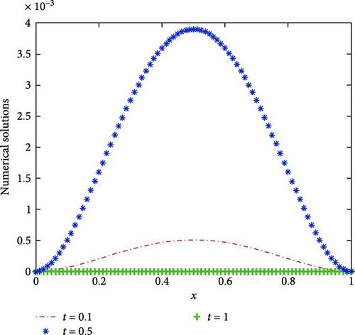
Let l_β = 1, r_β = 3, l_γ = 5, r_γ = 7, and m = n = 2. Using the proposed numerical scheme to solve Example 1, the numerical results obtained under different (α, β, γ) and (λ₁, λ₂, λ₃) and step sizes (τ = h) are shown in Table 1. From Table 1, we can find that the numerical results are consistent with the theoretical analysis. The images of the numerical solutions are also shown in Figures 1 and 2.

Table 1. Numerical results at time t = 1 under different conditions.

(α, β, γ)	h = τ	λ₁ = 0.1		λ₁ = 1
		λ₂ = 0.2		λ₂ = 2
		λ₃ = 1		λ₃ = 3
			Order		Order
(0.2, 0.5, 1.8)	1/10	7.6792e−07	—	2.0326e−07	—
	1/20	2.1300e−07	1.8501	8.2863e−08	1.2945
	1/40	5.5403e−08	1.9428	2.4849e−08	1.7375
	1/80	1.3988e−08	1.9858	6.6194e−09	1.9084

(0.2, 0.8, 1.5)	1/10	1.2185e−06	—	1.1711e−06	—
	1/20	3.7007e−07	1.7192	3.3470e−07	1.8069
	1/40	9.8470e−08	1.9100	8.4278e−08	1.9896
	1/80	2.4816e−08	1.9884	2.1220e−08	1.9897

(0.5, 0.2, 1.8)	1/10	3.4879e−06	—	2.2053e−06	—
	1/20	9.7554e−07	1.8381	7.8275e−07	1.4944
	1/40	2.5566e−07	1.9320	2.2514e−07	1.7977
	1/80	6.5053e−08	1.9745	5.9587e−08	1.9178

(0.5, 0.8, 1.2)	1/10	3.3155e−06	—	2.8933e−05	—
	1/20	1.7777e−06	0.8992	1.2486e−05	1.2124
	1/40	5.7928e−07	1.6177	3.5922e−06	1.7974
	1/80	1.5799e−07	1.8744	9.2582e−07	1.9561

(0.8, 0.2, 1.5)	1/10	1.8438e−05	—	1.1337e−05	—
	1/20	5.5050e−06	1.7439	4.6972e−06	1.2712
	1/40	1.4726e−06	1.9024	1.4374e−06	1.7083
	1/80	3.7748e−07	1.9639	3.8962e−07	1.8833

(0.8, 0.5, 1.2)	1/10	1.8675e−05	—	4.4963e−05	—
	1/20	6.9562e−06	1.4247	2.5007e−05	0.8464
	1/40	2.0591e−06	1.7563	7.7313e−06	1.6935
	1/80	5.4925e−07	1.9065	2.0174e−06	1.9382

Example 2. Consider the following tempered fractional convection–diffusion equations:

where 0 < α < 1, 1 < β < 2, and

, and the linear source term is as follows:

The exact solution is

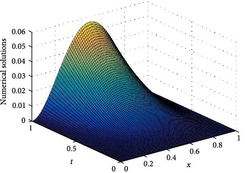
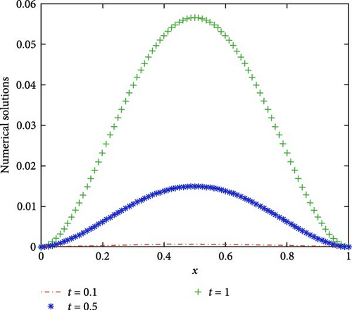
Let l_β = 1, r_β = 2, l_γ = 3, r_γ = 4, and m = n = 2. Using the proposed numerical scheme to solve Example 2, the error, observation order, and CPU time obtained under different (α, β, γ) and step sizes (τ = h) are shown in Table 2. We can see from Table 2 that the numerical results are in agreement with the theoretical analysis. The images of the numerical solutions are also shown in Figures 3 and 4.

Details are in the caption following the image — **Figure 1**
Open in figure viewer PowerPoint

Graph of numerical solutions for Example 1: α = 0.8, β = 0.5, γ = 1.2, λ₁ = 0.1, λ₂ = 0.2, λ₃ = 1, M = N = 80.

Table 2. Numerical results and CPU running time at time t = 1 under different conditions.

(α, β, γ)	λ₁ = 0.1	λ₂ = 0.2	λ₃ = 0.5	CPU time(s)
(α, β, γ)	h = τ		Order	CPU time(s)
(0.2, 0.5, 1.8)	1/10	9.0027e−04	—	0.0538
	1/20	2.2508e−04	1.9999	0.1525
	1/40	5.4294e−05	2.0516	0.1541
	1/80	1.2889e−05	2.0747	0.3635

(0.2, 0.8, 1.5)	1/10	4.9078e−04	—	0.0535
	1/20	1.4967e−04	1.7133	0.1527
	1/40	4.0599e−05	1.8823	0.1553
	1/80	1.0609e−05	1.9362	0.3473

(0.5, 0.2, 1.8)	1/10	6.9563e−04	—	0.0545
	1/20	1.6891e−04	2.0421	0.1524
	1/40	3.9553e−05	2.0944	0.1551
	1/80	9.1303e−06	2.1151	0.3538

(0.5, 0.8, 1.2)	1/10	1.9091e−03	—	0.0547
	1/20	4.5829e−04	2.0586	0.1539
	1/40	1.1162e−04	2.0377	0.1552
	1/80	2.7968e−05	1.9978	0.3558

(0.8, 0.2, 1.5)	1/10	5.8513e−04	—	0.0539
	1/20	1.6304e−04	1.8435	0.1525
	1/40	4.6538e−05	1.8087	0.1555
	1/80	1.3188e−05	1.8192	0.3538

(0.8, 0.5, 1.2)	1/10	2.7043e−03	—	0.0544
	1/20	7.0178e−04	1.9462	0.1547
	1/40	1.7523e−04	2.0018	0.1564
	1/80	4.3786e−05	2.0007	0.3556

6. Conclusions

In this paper, we focus on the higher-order numerical scheme of tempered fractional convection–diffusion equation with time Caputo-tempered fractional derivative. Different from the existing work, the discretization of time Caputo-tempered fractional derivative is directly performed by using the second-order tempered weighted and shifted Grünwald difference operator, and the proof of stability and convergence is simpler. Finally, some numerical examples are given to verify the effectiveness of the proposed scheme. In the following research work, we expect to propose high-order quasi-compact schemes for the tempered fractional diffusion equation and even the tempered fractional convection–diffusion equation. In addition, we hope to extend the problem with smooth solutions to the case of nonsmooth solutions and to develop the efficient numerical schemes.

Conflicts of Interest

The authors declare no conflicts of interest.

Author Contributions

Lizan Wang and Jianxin Li contributed equally to this work.

Funding

This research is supported by the Xinjiang University of Political Science and Law President Fund (XZZK2024008).

Acknowledgments

This research is supported by the Xinjiang University of Political Science and Law President Fund (XZZK2024008).

Open Research

Data Availability Statement

The data that support the findings of this study are available from the corresponding author upon reasonable request.

References

1 Baeumer B. and Meerschaert M. M., Tempered Stable Lvy Motion and Transient Super-Diffusion, Journal of Computational and Applied Mathematics. (2010) 233, no. 10, 2438–2448, https://doi.org/10.1016/j.cam.2009.10.027, 2-s2.0-73449087933.
10.1016/j.cam.2009.10.027
Google Scholar
2 Li C. and Deng W., High Order Schemes for the Tempered Fractional Diffusion Equations, Advances in Computational Mathematics. (2016) 42, no. 3, 543–572, https://doi.org/10.1007/s10444-015-9434-z, 2-s2.0-84944524237.
10.1007/s10444-015-9434-z
Web of Science® Google Scholar
3 Sabzikar F., Meerschaert M. M., and Chen J., Tempered Fractional Calculus, Journal of Computational Physics. (2015) 293, 14–28, https://doi.org/10.1016/j.jcp.2014.04.024, 2-s2.0-84899037917.
10.1016/j.jcp.2014.04.024
PubMed Web of Science® Google Scholar
4 Weilbeer M., Efficient Numerical Methods for Fractional Differential Equations and Their Analytical Background, 2005, https://api.semanticscholar.org/CorpusID:125828993.
Google Scholar
5 Benson D. A., Wheatcraft S. W., and Meerschaert M. M., Application of a Fractional Advection-Dispersion Equation, Water Resources Research. (2000) 36, no. 6, 1403–1412, https://doi.org/10.1029/2000WR900031, 2-s2.0-0034032484.
10.1029/2000WR900031
Web of Science® Google Scholar
6 Barkai E., Garini Y., and Metzler R., Strange Kinetics of Single Molecules in Living Cells, Physics Today. (2012) 65, no. 8, 29–35, https://doi.org/10.1063/PT.3.1677, 2-s2.0-84868254061.
10.1063/PT.3.1677
CAS Web of Science® Google Scholar
7 Scalas E., Gorenflo R., and Mainardi F., Fractional Calculus and Continuous-Time Finance, Physica A: Statistical Mechanics and its Applications. (2000) 284, no. 1–4, 376–384, https://doi.org/10.1016/S0378-4371(00)00255-7, 2-s2.0-0034275979.
10.1016/S0378-4371(00)00255-7
Web of Science® Google Scholar
8 Cushman J. H. and Ginn T. R., Fractional Advection-Dispersion Equation: A Classical Mass Balance With Convolution-Fickian Flux, Water Resources Research. (2000) 36, no. 12, 3763–3766, https://doi.org/10.1029/2000WR900261, 2-s2.0-0034515585.
10.1029/2000WR900261
Web of Science® Google Scholar
9 Meerschaert M. M., Zhang Y., and Baeumer B., Tempered Anomalous Diffusion in Heterogeneous Systems, Geophysical Research Letters. (2008) 35, no. 17, https://doi.org/10.1029/2008GL034899, 2-s2.0-57049164298, L17403.
10.1029/2008GL034899
Web of Science® Google Scholar
10 Hilfer R., Applications of Fractional Calculus in Physics, 2000, World Scientific, https://doi.org/10.1142/3779.
10.1142/3779
Google Scholar
11 Metzler R. and Klafter J., The Restaurant at the End of the Random Walk: Recent Developments in the Description of Anomalous Transport by Fractional Dynamics, Journal of Physics A: Mathematical and General. (2004) 37, no. 31, R161–R208, https://doi.org/10.1088/0305-4470/37/31/R01, 2-s2.0-4043151477.
10.1088/0305-4470/37/31/R01
Web of Science® Google Scholar
12 Zhang Y., Benson D. A., and Reeves D. M., Time and Space Nonlocalities Underlying Fractional-Derivative Models: Distinction and Literature Review of Field Applications, Advances in Water Resources. (2009) 32, no. 4, 561–581, https://doi.org/10.1016/j.advwatres.2009.01.008, 2-s2.0-62349097511.
10.1016/j.advwatres.2009.01.008
CAS Web of Science® Google Scholar
13 Çelik C. and Duman M., Crank-Nicolson Method for the Fractional Diffusion Equation With the Riesz Fractional Derivative, Journal of Computational Physics. (2012) 231, no. 4, 1743–1750, https://doi.org/10.1016/j.jcp.2011.11.008, 2-s2.0-84855207635.
10.1016/j.jcp.2011.11.008
Web of Science® Google Scholar
14 Tadjeran C., Meerschaert M. M., and Scheffler H.-P., A Second-Order Accurate Numerical Approximation for the Fractional Diffusion Equation, Journal of Computational Physics. (2006) 213, no. 1, 205–213, https://doi.org/10.1016/j.jcp.2005.08.008, 2-s2.0-31744438550.
10.1016/j.jcp.2005.08.008
Web of Science® Google Scholar
15 Hu D. and Cao X., A Fourth-Order Compact ADI Scheme for Two-Dimensional Riesz Space Fractional Nonlinear Reaction-Diffusion Equation, International Journal of Computer Mathematics. (2020) 97, no. 9, 1928–1948, https://doi.org/10.1080/00207160.2019.1671587, 2-s2.0-85073991337.
10.1080/00207160.2019.1671587
Web of Science® Google Scholar
16 Liu F., Zhuang P., and Burrage K., Numerical Methods and Analysis for a Class of Fractional Advection-Dispersion Models, Computers & Mathematics With Applications. (2012) 64, no. 10, 2990–3007, https://doi.org/10.1016/j.camwa.2012.01.020, 2-s2.0-84868214613.
10.1016/j.camwa.2012.01.020
Web of Science® Google Scholar
17 Zhou H., Tian W. Y., and Deng W., Quasi-Compact Finite Difference Schemes for Space Fractional Diffusion Equations, Journal of Scientific Computing. (2013) 56, no. 1, 45–66, https://doi.org/10.1007/s10915-012-9661-0, 2-s2.0-84877620868.
10.1007/s10915-012-9661-0
Web of Science® Google Scholar
18 Meerschaert M. M. and Tadjeran C., Finite Difference Approximations for Fractional Advection-Dispersion Equations, Journal of Computational and Applied Mathematics. (2004) 172, no. 1, 65–77, https://doi.org/10.1016/j.cam.2004.01.033, 2-s2.0-4444368867.
10.1016/j.cam.2004.01.033
Google Scholar
19 Hooshmandasl M. R., Heydari M. H., and Cattani C., Numerical Solution of Fractional Sub-Diffusion and Time-Fractional Diffusion-Wave Equations via Fractional-Order Legendre Functions, The European Physical Journal Plus. (2016) 131, no. 8, https://doi.org/10.1140/epjp/i2016-16268-2, 2-s2.0-84982861785, 268.
10.1140/epjp/i2016-16268-2
Google Scholar
20 Hang T., Zhou Z., Pan H., and Wang Y., The Conservative Characteristic Difference Method and Analysis for Solving Two-Sided Space-Fractional Advection-Diffusion Equations, Numerical Algorithms. (2023) 92, no. 3, 1723–1755, https://doi.org/10.1007/s11075-022-01363-2.
10.1007/s11075-022-01363-2
Google Scholar
21 Tian W. Y., Zhou H., and Deng W., A Class of Second Order Difference Approximations for Solving Space Fractional Diffusion Equations, Mathematics of Computation. (2015) 84, no. 294, 1703–1727, https://doi.org/10.1090/S0025-5718-2015-02917-2, 2-s2.0-84922436652.
10.1090/S0025-5718-2015-02917-2
Web of Science® Google Scholar
22 Zhang Y., Li Q., and Ding H., High-Order Numerical Approximation Formulas for Riemann-Liouville (Riesz) Tempered Fractional Derivatives: Construction and Application (I), Applied Mathematics and Computation. (2018) 329, 432–443, https://doi.org/10.1016/j.amc.2018.02.023, 2-s2.0-85042667590.
10.1016/j.amc.2018.02.023
Web of Science® Google Scholar
23 Hao Z.-P., Sun Z.-Z., and Cao W.-R., A Fourth-Order Approximation of Fractional Derivatives With Its Applications, Journal of Computational Physics. (2015) 281, 787–805, https://doi.org/10.1016/j.jcp.2014.10.053, 2-s2.0-84919897670.
10.1016/j.jcp.2014.10.053
Web of Science® Google Scholar
24 Lin Y. and Xu C., Finite Difference/Spectral Approximations for the Time-Fractional Diffusion Equation, Journal of Computational Physics. (2007) 225, no. 2, 1533–1552, https://doi.org/10.1016/j.jcp.2007.02.001, 2-s2.0-34547548712.
10.1016/j.jcp.2007.02.001
Web of Science® Google Scholar
25 Sun Z.-Z. and Wu X., A Fully Discrete Difference Scheme for a Diffusion-Wave System, Applied Numerical Mathematics. (2006) 56, no. 2, 193–209, https://doi.org/10.1016/j.apnum.2005.03.003, 2-s2.0-30744474991.
10.1016/j.apnum.2005.03.003
Web of Science® Google Scholar
26 Gao G.-H., Sun Z.-Z., and Zhang H.-W., A New Fractional Numerical Differentiation Formula to Approximate the Caputo Fractional Derivative and Its Applications, Journal of Computational Physics. (2014) 259, 33–50, https://doi.org/10.1016/j.jcp.2013.11.017, 2-s2.0-84890165820.
10.1016/j.jcp.2013.11.017
Web of Science® Google Scholar
27 Alikhanov A. A., A New Difference Scheme for the Time Fractional Diffusion Equation, Journal of Computational Physics. (2015) 280, 424–438, https://doi.org/10.1016/j.jcp.2014.09.031, 2-s2.0-84908329447.
10.1016/j.jcp.2014.09.031
Web of Science® Google Scholar
28 Cen D., Wang Z., and Mo Y., Second Order Difference Schemes for Time-Fractional KdV-Burgers’ Equation With Initial Singularity, Applied Mathematics Letters. (2021) 112, https://doi.org/10.1016/j.aml.2020.106829, 106829.
10.1016/j.aml.2020.106829
Web of Science® Google Scholar
29 Chawla R., Kumar D., and Singh S., A Second-Order Scheme for the Generalized Time-Fractional Burgers’ Equation, Journal of Computational and Nonlinear Dynamics. (2024) 19, no. 1, https://doi.org/10.1115/1.4063792, 011001.
10.1115/1.4063792
Google Scholar
30 Hao Z., Cao W., and Lin G., A Second-Order Difference Scheme for the Time Fractional Substantial Diffusion Equation, Journal of Computational and Applied Mathematics. (2017) 313, 54–69, https://doi.org/10.1016/j.cam.2016.09.006, 2-s2.0-84989158676.
10.1016/j.cam.2016.09.006
Google Scholar
31 Ding H. and Li C., A High-Order Algorithm for Time-Caputo-Tempered Partial Differential Equation With Riesz Derivatives in Two Spatial Dimensions, Journal of Scientific Computing. (2019) 80, no. 1, 81–109, https://doi.org/10.1007/s10915-019-00930-5, 2-s2.0-85062698212.
10.1007/s10915-019-00930-5
Google Scholar
32 Ahmed H. M., Hafez R. M., and Abd-Elhameed W. M., A Computational Strategy for Nonlinear Time-Fractional Generalized Kawahara Equation Using New Eighth-Kind Chebyshev Operational Matrices, Physica Scripta. (2024) 99, no. 4, https://doi.org/10.1088/1402-4896/ad3482, 045250.
10.1088/1402-4896/ad3482
CAS Google Scholar
33 Hafez R. M., Youssri Y. H., and Atta A. G., Jacobi Rational Operational Approach for Time-Fractional Sub-Diffusion Equation on a Semi-Infinite Domain, Contemporary Mathematics. (2023) 4, 853–876, https://doi.org/10.37256/cm.4420233594.
10.37256/cm.4420233594
Google Scholar
34 Hafez R. M., Hammad M., and Doha E. H., Fractional Jacobi Galerkin Spectral Schemes for Multi-Dimensional Time Fractional Advection-Difusion-Reaction Equations, Engineering With Computers. (2022) 38, no. S1, 841–858, https://doi.org/10.1007/s00366-020-01180-y.
10.1007/s00366-020-01180-y
Google Scholar
35 Youssri Y. H., Hafez R. M., and Atta A. G., An Innovative Pseudo-Spectral Galerkin Algorithm for the Time-Fractional Tricomi-Type Equation, Physica Scripta. (2024) 99, no. 10, https://doi.org/10.1088/1402-4896/ad74ad, 105238.
10.1088/1402-4896/ad74ad
CAS Google Scholar
36 Cartea Á. and del-Castillo-Negrete D., Fluid Limit of the Continuous-Time Random Walk With General Lvy Jump Distribution Functions, Physical Review E. (2007) 76, no. 4, https://doi.org/10.1103/physreve.76.041105, 2-s2.0-35248828149, 041105.
10.1103/physreve.76.041105
CAS Google Scholar
37 Chen M. and Deng W., High Order Algorithms for the Fractional Substantial Diffusion Equation With Truncated Lévy Flights, SIAM Journal on Scientific Computing. (2015) 37, no. 2, A890–A917, https://doi.org/10.1137/14097207X, 2-s2.0-84928941421.
10.1137/14097207X
Google Scholar
38 Zhao Y.-L., Huang T.-Z., Gu X.-M., and Luo W.-H., A Fast Second-Order Implicit Difference Method for Time-Space Fractional Advection-Diffusion Equation, Numerical Functional Analysis and Optimization. (2020) 41, no. 3, 257–293, https://doi.org/10.1080/01630563.2019.1627369, 2-s2.0-85067874248.
10.1080/01630563.2019.1627369
Google Scholar
39 Hanert E. and Piret C., A Chebyshev Pseudospectral Method to Solve the Space-Time Tempered Fractional Diffusion Equation, SIAM Journal on Scientific Computing. (2014) 36, no. 4, A1797–A1812, https://doi.org/10.1137/130927292, 2-s2.0-84928953692.
10.1137/130927292
Web of Science® Google Scholar
40 Yu Y., Deng W., Wu Y., and Wu J., Third Order Difference Schemes (Without Using Points Outside of the Domain) for One Sided Space Tempered Fractional Partial Differential Equations, Applied Numerical Mathematics. (2017) 112, 126–145, https://doi.org/10.1016/j.apnum.2016.10.011, 2-s2.0-84993967154.
10.1016/j.apnum.2016.10.011
Web of Science® Google Scholar
41 Qiu Z., Fourth-Order High-Precision Algorithms for One-Sided Tempered Fractional Diffusion Equations, AIMS Mathematics. (2024) 9, no. 10, 27102–27121.
10.3934/math.20241318
Google Scholar
42 Moghaddam B. P., Machado J. A. T., and Babaei A., A Computationally Efficient Method for Tempered Fractional Differential Equations With Application, Computational and Applied Mathematics. (2018) 37, no. 3, 3657–3671, https://doi.org/10.1007/s40314-017-0522-1, 2-s2.0-85049795329.
10.1007/s40314-017-0522-1
Web of Science® Google Scholar
43 Hu D. and Cao X., The Implicit Midpoint Method for Riesz Tempered Fractional Diffusion Equation With a Nonlinear Source Term, Advances in Difference Equations. (2019) 2019, https://doi.org/10.1186/s13662-019-1990-y, 2-s2.0-85061811895, 66.
10.1186/s13662-019-1990-y
Google Scholar
44 Zhang H., Liu F., Turner I., and Chen S., The Numerical Simulation of the Tempered Fractional Black-Scholes Equation for European Double Barrier Option, Applied Mathematical Modelling. (2016) 40, no. 11-12, 5819–5834, https://doi.org/10.1016/j.apm.2016.01.027, 2-s2.0-84969326965.
10.1016/j.apm.2016.01.027
Web of Science® Google Scholar
45 Feng L., Liu F., and Anh V. V., Galerkin Finite Element Method for a Two-Dimensional Tempered Time-Space Fractional Diffusion Equation With Application to a Bloch-Torrey Equation Retaining Larmor Precession, Mathematics and Computers in Simulation. (2023) 206, 517–537, https://doi.org/10.1016/j.matcom.2022.11.024.
10.1016/j.matcom.2022.11.024
Google Scholar
46 Feng L., Liu F., Anh V. V., and Qin S., Analytical and Numerical Investigation on the Tempered Time-Fractional Operator With Application to the Bloch Equation and the Two-Layered Problem, Nonlinear Dynamics. (2022) 109, no. 3, 2041–2061, https://doi.org/10.1007/s11071-022-07561-w.
10.1007/s11071-022-07561-w
Google Scholar
47 Dehghan M. and Abbaszadeh M., A Finite Difference/Finite Element Technique With Error Estimate for Space Fractional Tempered Diffusion-Wave Equation, Computers & Mathematics With Applications. (2018) 75, no. 8, 2903–2914, https://doi.org/10.1016/j.camwa.2018.01.020, 2-s2.0-85042613734.
10.1016/j.camwa.2018.01.020
Google Scholar
48 Dehghan M., Abbaszadeh M., and Deng W., Fourth-Order Numerical Method for the Space-Time Tempered Fractional Diffusion-Wave Equation, Applied Mathematics Letters. (2017) 73, 120–127, https://doi.org/10.1016/j.aml.2017.04.011, 2-s2.0-85019955614.
10.1016/j.aml.2017.04.011
Web of Science® Google Scholar
49 Deng W. H. and Zhang Z. J., Numerical Schemes of the Time Tempered Fractional Feynman-Kac Equation, Computers & Mathematics With Applications. (2017) 73, no. 6, 1063–1076, https://doi.org/10.1016/j.camwa.2016.12.017, 2-s2.0-85008622448.
10.1016/j.camwa.2016.12.017
Google Scholar
50 Luo W.-H., Gu X.-M., Yang L., and Meng J., A Lagrange-Quadratic Spline Optimal Collocation Method for the Time Tempered Fractional Diffusion Equation, Mathematics and Computers in Simulation. (2021) 182, 1–24, https://doi.org/10.1016/j.matcom.2020.10.016.
10.1016/j.matcom.2020.10.016
Google Scholar
51 Zhao Y.-L., Zhu P.-Y., Gu X.-M., Zhao X.-L., and Jian H.-Y., A Preconditioning Technique for All-at-Once System from the Nonlinear Tempered Fractional Diffusion Equation, Journal of Scientific Computing. (2020) 83, no. 1, https://doi.org/10.1007/s10915-020-01193-1, 10.
10.1007/s10915-020-01193-1
Google Scholar
52 Qiu Z., An Unconditionally Stable Numerical Method for Space Tempered Fractional Convection-Diffusion Models, Journal of Mathematics. (2024) 2024, 6710903.
10.1155/2024/6710903
Google Scholar
53 Quarteroni A. and Valli A., Numerical Approximation of Partial Differential Equations, 1994, Springer, https://doi.org/10.1007/978-3-540-85268-1.
10.1007/978-3-540-85268-1
Google Scholar

All articles

A Simple and Effective Second-Order Numerical Algorithm for Tempered Fractional Differential Equation With Time Caputo-Tempered Fractional Derivative

Abstract

1. Introduction

2. Preliminary

3. Numerical Discretization

4. Stability and Convergence Analysis

5. Numerical Examples

6. Conclusions

Conflicts of Interest

Author Contributions

Funding

Acknowledgments

Open Research

Data Availability Statement

References

Figures

References

Information

About Wiley Online Library

Help & Support

Opportunities

Connect with Wiley

A Simple and Effective Second-Order Numerical Algorithm for Tempered Fractional Differential Equation With Time Caputo-Tempered Fractional Derivative

Abstract

1. Introduction

2. Preliminary

3. Numerical Discretization

4. Stability and Convergence Analysis

5. Numerical Examples

6. Conclusions

Conflicts of Interest

Author Contributions

Funding

Acknowledgments

Open Research

Data Availability Statement

References

Figures

References

Related

Information