1. Introduction

In wireless multihop networks, such as wireless mesh networks and wireless body sensor networks, link quality (LQ) is an important quality indicator of wireless data transmission channels [1, 2]. LQ prediction allows the transmitter to learn the quality of data transmission channels in advance and adjust transmission policies in time. Therefore, the performance of higher-layer applications, such as routing, power control, quality of service, and energy consumption [3–5], relies heavily on the high accuracy of LQ prediction. Routing protocols, for example, if the LQ is available before making routing decision, the weak connections can be eliminated. As a result, the stability and the robustness of routing protocols are improved. Therefore, LQ prediction has great significance in wireless multihop networks.

However, in most wireless networks, the LQ between two wireless nodes is hard to accurately predict. This is because the radio wave propagation experiences reflection, blocking, scattering, and diffraction, which has an adverse effect on the transmitted signal that travels in the wireless channel [6, 7]. Commonly, the received wireless signal consists of two parts, one of which is distance-dependent path loss and the other is small-scale fading [8]. Because of the randomness of small-scale fading, the received signal level is unpredictable to some extent. The log-normal shadow fading channel model [9], for example, the stochastic fading component is chosen from a normal probability density function. Meanwhile, the mobility of nodes in wireless multihop networks brings additional randomness in received signal level. Currently, machine learning algorithms are not able to make accurate predictions with respect to objective uncertainties, and the accuracy of LQ prediction models depends on the uncertainty of wireless transmission.

In order to weaken the influence of randomness of wireless transmission on the performance of LQ prediction, researchers have proposed a large number of LQ prediction models for different application scenarios and different network models. Generally, in LQ prediction models, there are mainly two types of LQ metrics [8], the physical metrics, such as received signal strength indicator (RSSI) and logical metrics, such as packet delivery ratio (PDR). The historical values of RSSI and PDR are usually used as input parameters of the prediction model. Unfortunately, both types of metrics are seriously affected by the randomness of the received signal and show a strong unpredictability at the receiving nodes. As we know, machine learning models are not capable of predicting purely random events. Therefore, accurate prediction of LQ becomes difficult or even impossible. However, most of these prediction models adopt similar research idea and focus on improving the prediction accuracy. As discussed above, due to the randomness of wireless transmission, the performance of these LQ prediction models is limited, and most studies have not conducted in-depth analysis on this issue. And, the majority of LQ applications are based on accurate predictions, such as LQ-based routing algorithms.

In this paper, we focus on common machine learning-based LQ prediction models, using physical and logical metrics as the input parameters, and study the impact of stochastic nature of wireless transmission on the performance of these prediction models. Firstly, we define a metric to measure the randomness of dataset and prediction model. Then, by deeply analyzing the performance of the prediction models, we analyze the impact of stochastic nature of wireless transmission on LQ prediction applications. Finally, we propose a mechanism for the application of a performance-limited prediction model in wireless multihop networks and analyze its advantages in improving network performance.

The rest of this paper is organized as follows. In Section 2, we design a machine learning-based wireless LQ prediction model and analyze the randomness of wireless transmission in detail. In Section 3, we analyze the performance of the proposed LQ prediction model with different values of randomness metric. Then, we mainly analyze the limitations of the prediction model from two aspects: the randomness of the prediction output and the accuracy of the prediction. In Section 4, the application of the performance-limited LQ prediction model is discussed. Finally, we conclude this paper in Section 5.

2. Related Works

At present, researchers have proposed a number of LQ prediction methods. These methods are basically divided into two main types, traditional optimization algorithms and machine learning-based models. In terms of traditional optimization algorithms, Meng [10] has proposed a Bernoulli sampling-based algorithm for the estimation of LQ. Xue, Hai, and Jian [11] have proposed a stable and sensitivity-adjustable evaluation algorithm based on exponential weighted moving average (EWMA) mathematical model. Traditional algorithms are difficult to solve the problem of timeliness of LQ prediction and are generally used to evaluate the LQ of the past period, such as EWMA.

Therefore, the mainstream LQ prediction methods are generally machine learning-based and can be divided into two types, the offline [12–17] and online [18–22] learning models. Most of the offline machine models consist of three steps: data collection, offline modeling, and online prediction. During the data collection phrase, the historical values of LQ metrics such as signal-to-noise ratio (SNR), RSSI, link quality indicator (LQI), frame error rate (FER), pack lost rate (FLR), and PDR are collected [12]. In the modelling phrase, the commonly used machine learning algorithms such as fuzzy logic, eXtreme Gradient Boosting (XGBoost), support vector regression (SVR), and neural networks (NN) [12] are often used as prediction models. Then, a combination of various LQ metrics is used as input parameters to train the prediction model. The output parameters mainly include the LQ level over a period of time, such as the package reception or the received signal strength for the next broadcast cycle. Finally, the trained model will be deployed in the actual network system to make the real-time LQ prediction.

Medaiyeseet and Lauf [6] have proposed an offline machine learning-based model that detects the operational environment of a robot using both radio and network parameters. The received signal strength, signal quality, expected transmission count, and communication distance are used as input parameters to train the model. Throughput potential ratio is used as prediction output. Lowrance and Lauf [13] have proposed fuzzy logic-based model, which aims to solve the LQ prediction and update problem in robot networks. The model is tested in a real-world robot network and shows good performance compared with the traditional linear regression approach. Other offline models such as improved fuzzy C-means clustering algorithm [14] and 4C [16] are proposed to make LQ prediction in wireless sensor networks (WSNs). Most of the LQ prediction models use similar inputs and outputs and have achieved good results in LQ prediction, which greatly improve the performance of wireless networks.

Moreover, in order to solve the mobility problem in wireless networks and achieve faster and more accurate LQ prediction, the researchers propose online learning models, such as incremental learning model [20]. Actually, in highly dynamic environment, such as vehicle-to-vehicle networks [19] and mobile robot networks [20], online learning models may have advantages over offline learning models in terms of prediction efficiency. In some other networks with low dynamic, such as mesh networks [21] and WSNs [22], online learning models can reduce computational complexity while ensuring prediction accuracy.

Consider the network model, most of the LQ prediction models are proposed for the static or quasistatic networks, such as mesh and WSNs [18–20, 23–25]. While for the networks with mobility, mobile ad-hoc networks (MANETs) [6, 16, 17, 26], for example, the additional network dynamic information is necessary for LQ prediction models. Otherwise, Gomes, Gomes, and Fonseca [23] and Varghese et al. [25] have proposed LQ prediction models for indoor and outdoor WSNs, respectively.

Whether it is an online learning model or an offline learning model, the prediction model mainly focuses on improving the LQ prediction accuracy. In anticipation, accurate LQ prediction results are expected to improve network stability and reliability by adjusting routing, data transmission and power control algorithms. However, wireless LQ prediction is more like the prediction of the randomness of wireless transmission, and it is difficult for traditional optimization algorithms or machine learning models to solve the prediction performance limitations caused by stochastic nature of wireless transmission. As far as we know, the latest researches on LQ prediction models have not conducted in-depth analysis on the limitations of prediction models under the influence of wireless transmission randomness.

3. Models

3.1. LQ Prediction Model

In this paper, we consider a WSN with random deployment of sensor nodes. In such network, the sensor nodes apply the LQ prediction models to get the quality of their wireless links in order to optimize routing, avoid disconnection, and make other network optimizations.

A sensor node periodically broadcasts HELLO packets to its neighbors and receives HELLO packets from its neighbors. In this way, the sensor node is easy to obtain the historical values of LQ metrics. The proposed model is shown in Figure 1.

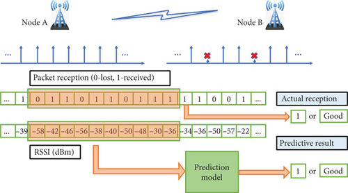
Suppose there are two nodes A and B; node A broadcasts HELLO packets periodically and node B receives these HELLO packets. Because of the fading characteristics of wireless wave propagation, HELLO packets may be lost at node B and the reception of HELLO packets has a certain randomness. In the proposed LQ prediction model, we use the historical information of HELLO packets for the previous K broadcast cycles as the input parameters to train the model. The historical information is the combination of both the logical and physical LQ metrics, the packet reception, and the corresponding RSSI.

In terms of prediction outputs (the labels), we mainly analyze two options. One is the HELLO packet reception for the next broadcast cycle, which is a two-class classification problem, and the other is the LQ level, which shows in Good (G), Medium Good (MG), Medium Bad (MB), and Bad (B), for the next period. Definitions of these labels are shown in Tables 1 and 2.

Table 1. Labels in two-class classification case. The packet reception for the next broadcast cycle: received or lost.

Label	Definition
Received	The HELLO packet is successfully received at the next broadcast cycle
Lost	The HELLO packet is lost at the next broadcast cycle

Table 2. Labels in four-class classification case. The LQ level for the next period: Good (G), Medium Good (MG), Medium Bad (MB), or Bad (B).

Label	Definition
G	Receive 3 HELLO packets during the following 3 broadcast cycles
MG	Receive 2 HELLO packets during the following 3 broadcast cycles
MB	Receive 1 HELLO packets during the following 3 broadcast cycles
B	Receive 0 HELLO packets during the following 3 broadcast cycles

For a more comprehensive analysis, we apply different machine learning models, such as NN, random forest (RF), decision tree (DT), XGBoost, and gradient boosting decision tree (GBDT). Then, we compare the performance of these models and choose a best model for in-depth analysis.

3.2. Link Model

In order to analyze the randomness of wireless link, we introduce a log-normal shadow fading model to describe the wireless link between two sensor nodes. Let d(a, b) denote the distance between node a and node b. Power transmitted at node a and power received at node b are denoted as p_t(a) and p_r(b), respectively. The signal attenuation is given by

$$ (1)

According to the log-normal shadow fading model, the signal attenuation comprises two components:

$$ (2)

β₁(a, b) is the deterministic geometric component, which is relative to the reference point (here 1 m), and it is given by

$$ (3)

with the path loss exponent α.

β₂ is the stochastic component, and it is chosen from a normal probability density function.

$$ (4)

with the standard deviation σ

For given p_t and p_r,th, we have the threshold attenuation

$$ (5)

When the signal attenuation β is less than the threshold attenuation, the receiver successfully receives the packet from the transmitter. With the increase of distance, the probability of successful reception decreases, which reflects the actual wireless environment. From Equation (13) in [5], we get the PDR of two nodes with distance d.

$$ (6)

where r₀ is the distance when the point-to-point PDR drops to 50%.

$$ (7)

In our simulation platform, we get the training dataset of the prediction model from wireless transmission between two nodes. The curve of p(d), which reflects the characteristics of wireless link, is shown in Figure 2.

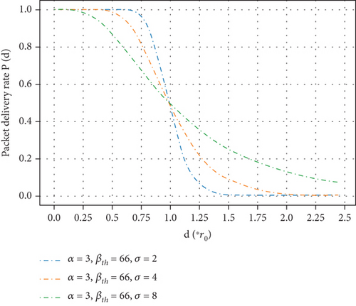
When the distance is relatively small, the PDR basically remains above 90%. When the distance is close to r₀, p(d) drops sharply which means that the link becomes unstable. When the distance continues to increase, the link becomes stable again and remains disconnected. Therefore, as shown in Figure 2, according to the distance between the neighbor nodes, the wireless channel can be roughly divided into three areas. Obviously, in the area around r₀, the link is the most unstable, and it is an important factor affecting the stability of the wireless multihop networks.

3.3. Randomness Metric

The randomness of wireless transmission is mainly reflected in two aspects: time and space. Consider the commonly used LQ metric, the RSSI, we have

$$ (8)

Let power transmitted at node a be p_t(a) = 50 mW, as shown in Figure 3, with the increase of distance, the RSSI shows a decreasing trend and strong randomness.

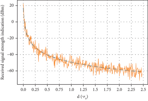
For two nodes with a given distance, r₀, for example, the change of the RSSI over time is shown in Figure 4.

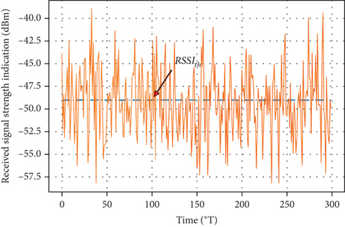
If we set a threshold of RSSI, the randomness of packet reception is shown in Figure 5.

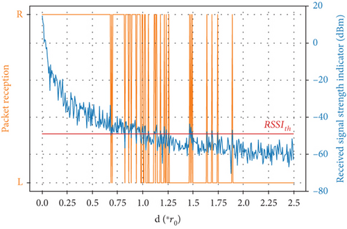
From Figure 5, we can see that if the distance between two nodes is around r₀, the packet reception shows strong randomness.

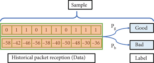
In our designed LQ prediction model, we use the historical information of HELLO packets as input parameters and use the packet reception for the next broadcast cycle or the LQ level for the next period as the output label. After we get the historical information (the data part of a sample), because of the randomness of wireless transmission, the label of this sample also shows a certain degree of randomness. As shown in Figure 6, the link condition is good for the past several broadcast cycles and has a high probability P_g of being marked as good. However, the LQ level label for this sample may also be marked as bad with a certain probability P_b.

In order to measure the randomness of a sample set, we define a randomness metric U. In the following sections, we analyze the relationship between the performance of LQ prediction model and randomness metric U. Suppose there are M different labels in the LQ prediction model, in order to train this model, we have the sample set S, which is given by

$$ (9)

where N is the number of samples in S, D_k is the data part of the k_th sample, t_k is the label of k_th sample, and S_i is the subset of S. Consider that the randomness of wireless links varies greatly in different environments, the samples in S_i are obtained from the nodes in the same environment and the subsets satisfy S_i∩S_j = Φ(i ≠ j). We define the label set T as

$$ (10)

Then, we have a sample s = (D, t) ∈ S, t ∈ T. The randomness metric U of sample set S is defined as

$$ (11)

where R_i(t) is the ratio of samples with label t in S_i.

$$ (12)

U_i(t) is the randomness metric of a given sample with label t in S_i.

$$ (13)

where p_tu is the probability that label t may mistakenly marked as label u. In LQ prediction application, for two nodes with distance d, the distribution of p_tu for the samples obtain from these two nodes are shown in Tables 3 and 4.

Table 3. Distribution of p_tu: two-class classification case.

t	u
	Lost	Received
Lost	1 − p(d)	p(d)
Received	1 − p(d)	p(d)

Table 4. Distribution of p_tu: four-class classification case.

t	u
	Good	Medium good	Medium bad	Bad
G	P(d)3	3(1 − P(d))P(d)2	3(1 − P(d))2P(d)	(1 − P(d))3
MG	P(d)3	3(1 − P(d))P(d)2	3(1 − P(d))2P(d)	(1 − P(d))3
MB	P(d)3	3(1 − P(d))P(d)2	3(1 − P(d))2P(d)	(1 − P(d))3
B	P(d)3	3(1 − P(d))P(d)2	3(1 − P(d))2P(d)	(1 − P(d))3

Then, we define the accuracy of the sample set as

$$ (14)

The randomness metric U of the sample set obtained from two nodes with different distance d is shown in Figure 7.

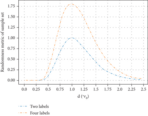
From Figure 7, we can see that when distance is around r₀, U reaches the maximum value, which is consistent with the actual link condition. The randomness metric U can well describe the randomness of a sample set.

4. Performance Analysis

In this section, we mainly analyze the performance of the designed LQ prediction models.

First of all, we built a simulation platform to model a network with multiple wireless nodes. Each node performs periodic broadcasting. By counting the nodes’ reception of broadcast packets, we get the historical sequence of packets received by sensor nodes in a certain time period, including the reception situation, signal strength, and other information. And training samples are extracted from the above sequence to train the LQ prediction models.

Let S_p denote the output sample set of the LQ prediction model when the input sample set is S. Similar to the definition of U(S), the randomness metric of the LQ prediction model is denoted as U_p(S).

In order to obtain the sample set for the proposed model, we built a simulation platform with two nodes whose distance is evenly distributed in (0, 2.5r₀). The simulation parameters and their values are shown in Table 5.

The performance of LQ prediction models with different machine learning algorithms are shown in Tables 6 and 7.

From Tables 6 and 7, we can see that the accuracy of each LQ prediction model is about the same. In two-class classification case, the NN model achieves the highest accuracy, while in the four-class classification case, the GBDT model achieves the highest accuracy. Nevertheless, the accuracy of the model is less than the reference maximum accuracy Acc_max. In terms of randomness, the randomness metric of LQ prediction model U_p is slightly larger than the randomness of sample set U, which means that the prediction model brings additional randomness while making LQ prediction, and the prediction output is still full of randomness. Therefore, in the applications using LQ prediction, affecting by the randomness of wireless transmission, high accuracy is not a necessary condition for the application. In the following analysis, we apply the NN and GBDT models for the two-class classification and four-class classification cases, respectively.

4.1. Performance in Static Randomness Environment

Considering the static wireless multihop networks, such as WSN and wireless mesh network, we obtain the samples from two nodes with the same distance, d = r₀, for example. Then, we train and test the LQ prediction model using these samples. The performance of LQ prediction models are shown in Figures 8, 9, 10, and 11.

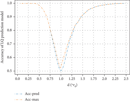
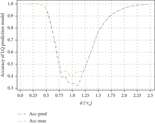
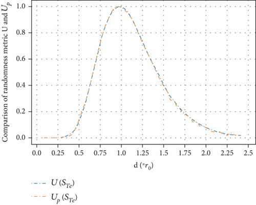
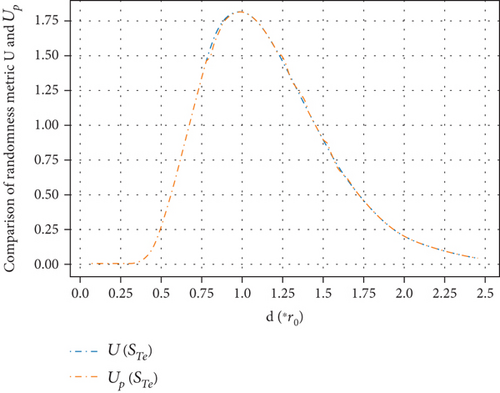
Figures 8 and 9 are the comparison of the accuracy of the prediction model and the reference maximum accuracy for two-class classification and four-class classification cases. Figures 10 and 11 are the comparison of randomness metric U_p and U for two-class classification and four-class classification cases, respectively. Comparing Figures 8 and 10 and Figures 9 and 11, we can see that with the increase of distance between two nodes, the randomness metric of the sample set and the accuracy of the prediction model have completely opposite trends. The prediction output has similar randomness metric as the sample set. When two nodes are very close or far apart, the accuracy of the prediction model is basically equal to the maximum accuracy. This is because when two nodes are very close or far apart, the randomness of wireless transmission is weak and the connection (or disconnection) is strong. As a result, the prediction model is easy to make accurate prediction.

However, when the distance between two nodes is getting close to r₀, the randomness of the samples increase sharply, as shown in Figures 10 and 11. Even when the best prediction model is applied, the prediction output still contains strong randomness and the output of the predictor is basically purely random. As shown in Figures 8 and 9, the accuracy of the prediction model has an unacceptably low accuracy when the distance is around r₀. Actually, in most wireless multihop networks, the LQ is almost unpredictable when the distance is around r₀. As a generally accepted fact that if such links are selected as relay links, the network becomes unstable.

4.2. Performance in Dynamic Randomness Environment

To further analyze the impact of the randomness on the performance of prediction model, we modify the value of randomness metric U by adjusting the composition of the sample set. Then, we train and test the LQ prediction model using the sample set with different randomness. In this paper, we apply the samples obtained from two nodes with distance dynamically distributed in (0.5r₀, 1.5r₀). We performed a total of 20 discrete experiments. Each experiment contains randomness metric U that are different from other experiments. The performance of LQ prediction models are shown in Figures 12, 13, 14, and 15.

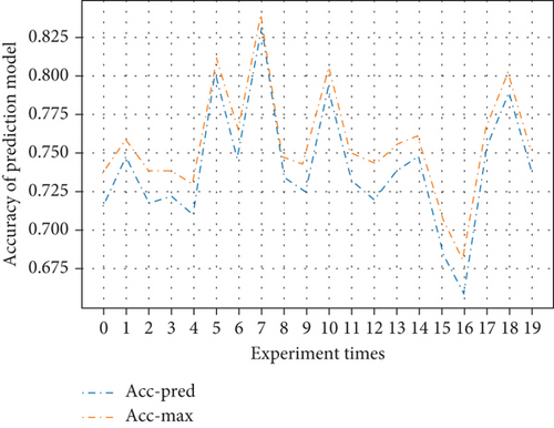
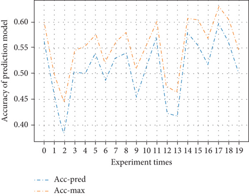
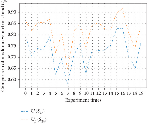
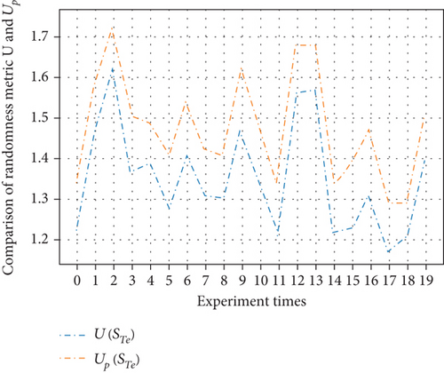
Figures 12 and 13 are the comparison of the accuracy of the prediction model and the reference maximum accuracy for two-class classification and four-class classification cases. In each experiment, the accuracy of the prediction model is slightly less than the reference maximum accuracy. The corresponding randomness metrics U and U_p are shown in Figures 14 and 15. From the figures, we know that the randomness of the prediction output is always stronger than the randomness of the input sample set, which means that the predictor brings additional randomness and the performance is limited.

In conclusion, since the randomness of the wireless transmission cannot be eliminated, the randomness of the prediction output cannot be eliminated either. The accuracy of the LQ prediction model is restricted by the randomness of the wireless link, and it is impossible to achieve a completely accurate prediction, especially at the edge of wireless coverage with strong randomness, the output of LQ prediction model becomes purely random.

5. Application of LQ Prediction Model

Although the prediction model is not accurate enough, we can still use the prediction output as the basis for whether the node processes the received data packets, which helps greatly to improve the stability of wireless transmission, especially the routing discovery process. The two-class classification case, for example, when the output of the prediction model is received, and the corresponding data packet is received at the next moment, the data packet will be processed. Otherwise, if the output is lost, even if the data packet is received at the next moment, it will be discarded.

By applying a two-class classification LQ prediction model, the packet reception of a node with LQ prediction model is shown in Figure 16. From the figure, we can see that the packet reception still has a certain randomness. However, compared with Figure 5, the randomness is weaker. Moreover, the strongest randomness occurs at the position where the distance is 0.8r₀. This is because in an area with strong randomness, when the prediction output is lost, the packet will be discarded even it is successfully received. Therefore, the PDR is further decreased. Actually, the prediction model helps to discard the accidentally received packets from the weak connections. The same regular pattern is also reflected in the curves of PDR in the cases before and after using prediction model.

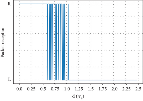
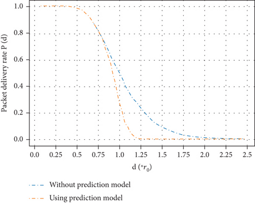
Figure 17 is the comparison of PDR before and after using the prediction model. After applying the prediction model, the PDR drops sharply, which means that the area with strong randomness is greatly reduced. In wireless multihop networks, this helps to reduce the use of unstable links and improve the network stability.

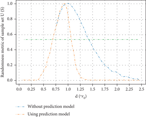
The comparison of randomness metric U before and after using the prediction model is shown in Figure 18. If we set the threshold of U as U_th = 0.5, it is easy to see that after using the prediction model, the area with strong randomness is greatly reduced.

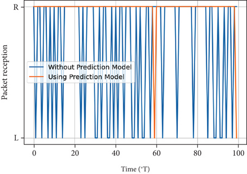
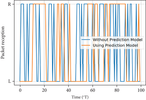
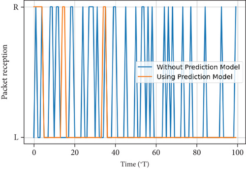
Figures 19, 20, and 21 are the packet receptions before and after using the prediction model at nodes with distances 0.8r₀, r₀, and 1.2r₀, respectively. It is intuitively shown that after using the prediction model, the packet reception becomes more stable in spite of the low prediction accuracy. When d = 0.8r₀, the prediction outputs are almost received, which means almost all received packets will be handed over to the upper layer. When d = 1.2r₀, the prediction outputs are almost lost. As a result, the receiver discards accidentally received packets.

Although the prediction model can effectively stabilize wireless links with strong randomness, the drawbacks are also obvious. The additional time costs and data transmission overhead are necessary to train an accurate prediction model. These overheads are acceptable when the capability of the nodes allows, and wireless LQ prediction can still improve the performance of wireless multihop networks.

6. Conclusion and Future Work

Disclosure

An older version of this work has been submitted as a preprint version to https://arxiv.org/abs/2110.08481 [21].

Conflicts of Interest

The authors declare no conflicts of interest.

Funding

This work was supported by the Provincial Science and Technology Innovation Strategy Special Project of Shaoguan City in 2023, Project No.: 230315116274818.