A fitted tension spline numerical scheme for a singularly perturbed parabolic problem (SPPP) with time delay is proposed. The presence of a small parameter ε as a multiple of the diffusion term leads to the suddenly changing behaviors of the solution in the boundary layer region. This results in a challenging duty to solve the problem analytically. Classical numerical methods cause spurious nonphysical oscillations unless an unacceptable number of mesh points is considered, which requires a large computational cost. To overcome this drawback, a numerical method comprising the backward Euler scheme in the time direction and the fitted spline scheme in the space direction on uniform meshes is proposed. To establish the stability and uniform convergence of the proposed method, an extensive amount of analysis is carried out. Three numerical examples are considered to validate the efficiency and applicability of the proposed scheme. It is proved that the proposed scheme is uniformly convergent of order one in both space and time. Further, the boundary layer behaviors of the solutions are given graphically.

1. Introduction

Delay differential equations in which its higher order derivative term is multiplied by a small perturbation parameter ε (0 < ε ≪ 1) and involving a delay term is known as singularly perturbed delay differential equations (SPDDEs). Physical phenomena such as gestation times, incubation periods, transport delays, and more can be represented by delays/lags [1]. SPDDEs have numerous applications in science and engineering, especially in biological, chemical, electronic, and transportation systems. Some of these include simulation of oil extraction from underground reservoirs [2], chemical processes, fluid flows, and water quality problems in river networks [3] and mechanical systems [4, 5]. A simplified example of a time-delayed mathematical model which is used in an automatic control system of a furnace to produce metal sheets is given as follows [6]:

(1)

where z denotes the temperature distribution in a metal sheet and f and v denote the heat source and the velocity with which the metal sheet is moving, respectively. Both f and v are dependent on the term z(s, t − ζ). The time delay of fixed length ζ is induced because of the finite speed of the controlling device. SPDDEs exhibit a boundary layer, where the solution changes rapidly as ε approaches zero. The boundary layer is a narrow region placed on the left or right side of the domain where the dependent variable undergoes very rapid [4]. Due to the existence of the boundary layer, solving SPDDEs using analytical or standard numerical schemes is a challenging task [7]. On the contrary, standard numerical methods cause spurious nonphysical oscillations in the numerical result unless an acceptable large number of mesh points are used; this is computationally not feasible [1, 8, 9]. To overcome these kinds of computational problems, one needs to look for a sound numerical method that converges uniformly regardless of ε.

Recently, a number of numerical methods have been conducted by different authors. Ayele, Tiruneh, and Derese [10] constructed a hybrid scheme of a proper combination of the midpoint upwind scheme in the outer layer region and the cubic spline method in the boundary layer region on the piecewise Shishkin mesh in the spatial direction. Das and Natesan [1] constructed a numerical scheme using the hybrid method on piecewise uniform Shishkin mesh in the space direction and an implicit Euler scheme in the temporal direction. Also, Govindarao and Mohapatra [11] constructed a numerical scheme using the hybrid scheme on Shishkin-type meshes in the space direction and an implicit trapezoidal scheme in the temporal direction. Gowrisankar and Natesan [12] proposed a numerical scheme using the upwind finite difference scheme on a piecewise uniform mesh. Salama and Al-Amery [13] constructed a numerical scheme comprising the Crank-Nicolson method for discretizing the time variable and the operator compact implicit (OCI) method in the spatial direction. Podila and Kumar [14] constructed a stable finite difference method that works on a uniform mesh and an adaptive mesh. The upwind finite difference method on Shishkin mesh is constructed in [15]. An adaptive mesh refinement approach is employed using the concept of entropy function in [16, 17]. An exponentially fitted finite difference method is considered in [9, 18]. The nonstandard finite difference scheme is considered in [19, 20] following Micken’s type discretization for the space derivatives. The authors in [7, 21] constructed the numerical techniques that work for large or small time delays. For the spatiotemporal delays differential equation, Ejere et al. [8] constructed a robust numerical technique. For the differential-difference equations, the authors in [22] developed the cubic spline in tension.

To the best of the authors’ knowledge, the fitted tension spline scheme has not been developed for solving singularly perturbed parabolic problems (SPPPs) with a time delay. As stated in [23], constructing uniformly convergent numerical methods regardless of ε is an active research area. This motivated us to look for a sound numerical method that converges uniformly regardless of ε. In this study, we developed a numerical scheme that comprises the backward Euler in the temporal direction and the fitted tension spline method in the space direction on uniform meshes. Thus, the main objective is to propose ε-uniform numerical method to treat SPPPs with a time delay.

In this study, the symbol C denotes a positive constant that is independent of ε and the mesh elements. The norm ‖.‖, denoted by , is the maximum norm.

2. Continuous Problem

On the domain

, we considered a SPPP of the form

(2)

where

0 < ε ≪ 1 and ζ > 0 are given constants; the functions κ(s), γ(s), μ(s, t), f(s, t) on and ψ_b(s, t), ψ_l(t), ψ_r(t) on η = η_l ∪ η_r ∪ η_b are sufficiently smooth and bounded to satisfy the following assumptions: (i) . (ii) . Under assumption (i), the solution of Problem (2) exhibits a boundary layer of width O(ε) along s = 1 [1], and under assumption (ii), Problem (2) exhibits a boundary layer of width O(ε) along s = 0 [16].

2.1. A Priori Bounds

The existence and uniqueness of the solution of Equation (2) can be ensured by the sufficient smoothness of ψ_b(s, t), ψ_l(t) and ψ_r(t), and the compatibility conditions of the corner points and the delay term [24] are stated below

( )

Setting ε = 0 in Equation (2) obtained the reduced problem. Under assumption (i), the reduced problem has the form

(3)

Under assumption (ii), the reduced problem has the form

(4)

Lemma 1 (see [1] maximum principle.)Let , given that ϕ(s, t) ≥ 0 ∀ (s, t) ∈ η and , then .

Lemma 2 (see [1], [11].)The solution z(s, t) of Equation (2) is estimated as

( )

Lemma 3 (see [1], [11].)The solution z(s, t) of Equation (2) is estimated as

( )

Lemma 4 (stability result). The solution z(s, t) of Equation (2) is estimated as

( )

where ϖ ≤ γ(s).

Proof 1. Determine the barrier functions χ^±(s, t) as χ^±(s, t) = ϖ⁻¹‖f‖ + max{|ψ_l(t)|, |ψ_b(s, t)|, |ψ_r(t)|} ± z(s, t), on the boundaries, we get χ^±(s, 0) = ϖ⁻¹‖f‖ + max{|ψ_l(t)|, |ψ_b(s, t)|, |ψ_r(t)|} ± z(s, 0) ≥ 0, χ^±(0, t) = ϖ⁻¹‖f‖ + max{|ψ_l(t)|, |ψ_b(0, t)|, |ψ_r(t)|} ± z(0, t) ≥ 0, and χ^±(1, t) = ϖ⁻¹‖f‖ + max{|ψ_l(t)|, |ψ_b(1, t)|, |ψ_r(t)|} ± z(1, t) ≥ 0. Then,

( )

which imply

Thus, from Lemma 1, χ^±(s, t) ≥ 0, such that,

( )

Therefore, the proof is done.

Lemma 5 (see [1], [13].)Let z(s, t) be the solution of Equation (2), then its derivative satisfies the estimate

(5)

for the boundary layer along s = 0 and

(6)

for the boundary layer along s = 1.

3. Numerical Method

3.1. The Time Semidiscretization

The time interval

is divided uniformly with M mesh points as

. As stated in [25], the delay parameter ζ is treated using the Taylor approximation. Using the backward Euler formula, we get

(7)

Equivalently, it is convenient to rewrite Equation (7) as

(8)

where

and

with the boundaries

(9)

Equations (8) and (9) can be rewritten as

(10)

with the boundaries

(11)

where Z(s) = Zⁿ(s) ≈ Z(s, t_n).

The local error estimate at the time step is given as e_n(s)≔z(s, t_n) − Zⁿ(s), n = 0(1)M.

Lemma 6. If and 0 ≤ k ≤ 2, then e_n is bounded as

( )

and the global error estimate

( )

Proof 2. The proof is considered in [26].

Lemma 7. For n = 0(1)M − 1, p = 0(1)4, then the derivative of the solution of Equations (8) and (9) satisfies the following bounds

(12)

for the boundary layer along s = 0 and

(13)

for the boundary layer along s = 1.

Proof 3. For the proof, see [27].

3.2. The Spatial Discretization

The space interval divided into N equally spaced nodes with mesh length h is given as 0 = s₀, s₁, ⋯, s_N = 1 and s_m = mh, m = 0(1)N.

3.2.1. Description of the Method

A function

that interpolates z(s) at the mesh points s_m that depends on the compression parameter τ and is reduced to a cubic spline on

as τ⟶0 is referred to as a parametric cubic spline function [28]. For each interval [s_m, s_m+1], m = 1(1)N − 1, the spline function

has the form

(14)

where

for τ > 0 is called cubic spline in tension. Putting

and from the homogeneous part of Equation (14), we get

(15)

for arbitrary constants

and

. Let the nonhomogeneous part be given as

( )

Thus, we have

(16)

where

and

. Using Equations (15) and (16), we obtain

(17)

From Equation (17), the arbitrary constants can be determined from the interpolation conditions

and

, then

(18)

The derivative of Equation (18) at (s_m, t_n) on the interval [s_m, s_m+1] is

(19)

and on the interval [s_m−1, s_m] is

(20)

Equating Equations (19) and (20) at the point s_m, we get

(21)

Simplifying Equation (21), we obtain

(22)

where α₁ = α⁻²(1 − αcschα) and α₂ = α⁻²(αcothα − 1). The continuity condition in Equation (22) ensures the continuity of the first derivative of

at interior nodes. Using

into Equation (10), we obtain

(23)

The local truncation error

obtained from Equation (22) is

( )

for any choice of α₁ and α₂ whose sum is 1/2. For the choice α₁ = 1/12 and α₂ = 5/12, we have

( )

Using Taylor series expansions, we approximate

and

(24)

Substituting Equation (24) into Equation (23) and substituting the resulting equation into Equation (22) and arranging, we get

(25)

where

3.2.2. Exponential Fitting Factor

Here, we find the exponential fitting factor σ to handle the effect of ε in the layer. As the theory of singularly perturbed problem given in [29] and Taylor’s series expansion of Z(s) about s = 0, the zero-order asymptotic solution of Equations (10) and (11) is given as

(26)

where ρ = h/ε.

Multiplying Equation (25) by σ with a term containing ε, we get

(27)

Thus, we consider two cases of the boundary layers:

Case 1. Left-end boundary layer for κ(s) < 0.

Multiplying Equation (27) by h and taking a limit as h⟶0, which gives

(28)

(29)

Substituting Equation (29) into Equation (28), we obtain

(30)

Case 2. Right-end boundary layer for κ(s) > 0.

Multiplying Equation (27) by h and taking a limit as h⟶0, which gives

(31)

(32)

Substituting Equation (32) into Equation (31), we obtain

(33)

Therefore, we take the variable exponential fitting factor

(34)

Therefore, inducing the obtained exponential fitting factor in Equation (34) into Equation (25) for m = 1(1)N − 1 and n = 1(1)M − 1, we obtain

(35)

where

( )

In the explicit form, we write Equation (35) as

(36)

where

(37)

3.3. Convergence Analysis

Lemma 8 (discrete comparison principle). There is a comparison function such that for m = 1(1)N − 1 and if and , then for m = 1(1)N.

Proof 4. For the proof, see [27, 30].

Lemma 9. The solution of Equation (35) satisfies

( )

where

Proof 5. Let and the barrier functions defined as . On the boundaries, we obtain and . On the discretized space domain s_m, m = 1(1)N − 1, we have

( )

From Lemma 8, we obtain . Hence, the desired bound is obtained.

From Taylor’s series approximation, yield the bounds

(38)

where

For the constants ρ > 0, C₁ and C₂, we have

(39)

Following Equation (39), we have

(40)

since α₁ + α₂ ≤ 1/2.

The next theorem provides the error bound in the spatial direction for the boundary layer along s = 1.

Theorem 1. Let Zⁿ(s) be the solution of Equations (8) and (9) and the solution of Equation (35) satisfies the following error estimate:

(41)

Proof 6. In the space direction, the error is given as

( )

Using the bounds in Equations (38) and (40), we obtain

( )

From Lemma 7, we obtain

( )

since ε⁻² ≤ ε⁻³ and the desired bound is obtained.

Lemma 10. For a fixed mesh and as ε⟶0, it gives

( )

where j = 1, 2, 3, ⋯ and s_m = mh, m = 1(1)N − 1.

Proof 7. The proof can be done by using L’Hospital’s rule. For the details, refer to [30].

Theorem 2. The solution of Equation (35) satisfies the following uniform error estimate:

( )

Proof 8. From Lemma 10 and Equation (41), we get

(42)

Hence, the result leads Using the sup over all ε ∈ (0, 1], we get

(43)

From Equation (42), we take two cases: when ε > h, the obtained method gives a second-order uniformly convergent. On the other hand, when ε ≪ h, the method is first-order uniformly convergent in the space direction.

Theorem 3. Let z and Z be the solutions of Equations (2) and (35), respectively. Then, the next uniform error estimate holds

(44)

Proof 9. The proof can be done following Lemma 6 and Theorem 2.

4. Numerical Results

The applicability of the proposed scheme is validated using three model examples. The numerical values are given for α₁ = 1/50 and α₂ = 24/50. For the unknown exact solution of the model examples, we use the double mesh principle for the numerical experiment [8, 9]. Therefore, the maximum pointwise error , ε-uniform error (E^N,M), the rate of convergence , and uniform rate of convergence (r^N,M) are calculated by , , and r^N,M = log2(E^N,M/E^2N,2M), respectively.

Example 1. Consider the problem [16] ∂z/∂t − ε(∂²z/∂s²) − ∂z/∂s + (1 + s²/2)z = t³ − z(s, t − ζ), (s, t) ∈ (0, 1) × (0, 2] with interval condition z(s, t) = 0, on (s, t) ∈ [0, 1] × [−ζ, 0] and the boundary conditions z(0, t) = 0 and z(1, t) = 0, t ∈ (0, 2].

Example 2. Consider the problem [1] ∂z/∂t − ε(∂²z/∂s²) + (2 − s²)∂z/∂s + sz(s, t) + z(s, t − ζ) = 10t²exp(−t)s(1 − s), (s, t) ∈ (0, 1) × (0, 2] with interval condition z(s, t) = 0 on (s, t) ∈ [0, 1] × [−ζ, 0] and the boundary conditions z(0, t) = 0 and z(1, t) = 0, t ∈ (0, 2].

Example 3. Consider the problem [15] ∂z/∂t − ε(∂²z/∂s²) + (2 − s²)∂z/∂s + (s + 1)(t + 1)z(s, t) + z(s, t − ζ) = 10t²exp(−t)s(1 − s), (s, t) ∈ (0, 1) × (0, 2] with interval condition z(s, t) = 0 on (s, t) ∈ [0, 1] × [−ζ, 0] and the boundary conditions z(0, t) = 0 and z(1, t) = 0, t ∈ [0, 2].

The , E^N,M, and the corresponding r^N,M of the proposed method are revealed in Tables 1–3 for each example, respectively, for different values of ε and N. These tables show that for every value of ε, monotonically decreases as the step sizes decrease, and as ε⟶0, the after showing growth and remains constant, demonstrating ε-uniform convergence of the developed method. On the other hand, the evaluated E^N,M and r^N,M applying the developed method are displayed in the last two rows, which support the theoretical result of the proposed method in the first-order in the space direction.

Table 1.

, E^N,M, and r^N,M for Example 1 for the case ζ = 0.5ε.

ε↓	16	32	64	128	256
	Number of intervals *N = M*
2⁻⁰	1.5462e − 02	7.3069e − 04	3.9085e − 04	2.0204e − 04	2.0272e − 04
2⁻²	1.5462e − 02	7.2071e − 03	3.8153e − 03	1.9627e − 03	9.9539e − 04
2⁻⁴	2.6720e − 02	1.5542e − 02	8.3415e − 03	4.3205e − 03	2.1985e − 03
2⁻⁶	3.3768e − 02	1.8165e − 02	1.0080e − 02	5.3565e − 03	2.7620e − 03
2⁻⁸	3.2640e − 02	1.9397e − 02	1.0778e − 02	5.2689e − 03	2.8084e − 03
2⁻¹⁰	3.2691e − 02	1.9261e − 02	1.0440e − 02	5.4740e − 03	2.8614e − 03
2⁻¹²	3.2705e − 02	1.9270e − 02	1.0443e − 02	5.4337e − 03	2.7717e − 03
2⁻¹⁴	3.2709e − 02	1.9272e − 02	1.0444e − 02	5.4343e − 03	2.7716e − 03
2⁻¹⁶	3.2709e − 02	1.9272e − 02	1.0444e − 02	5.4345e − 03	2.7717e − 03
2⁻¹⁸	3.2710e − 02	1.9273e − 02	1.0444e − 02	5.4345e − 03	2.7717e − 03
2⁻²⁰	3.2710e − 02	1.9273e − 02	1.0444e − 02	5.4345e − 03	2.7717e − 03
E^N,M	3.3768e − 02	1.9397e − 02	1.0778e − 02	5.4740e − 03	2.8614e − 03
r^N,M	0.7998	0.8477	0.9774	0.9359	—

Table 2.

, E^N,M, and r^N,M for Example 2 for the case ζ = 0.5ε.

ε↓	16	32	64	128	256
	Number of intervals *N = M*
2⁻⁰	2.3794e − 04	4.2183e − 05	3.7942e − 06	4.8888e − 06	3.6409e − 06
2⁻²	5.0365e − 04	1.1446e − 04	1.1509e − 04	7.2877e − 05	4.0330e − 05
2⁻⁴	1.3155e − 03	3.3537e − 04	2.4985e − 04	1.4687e − 04	7.9172e − 05
2⁻⁶	4.6137e − 03	1.7222e − 03	6.5369e − 04	2.7011e − 04	1.2039e − 04
2⁻⁸	6.3373e − 03	4.5453e − 03	2.0441e − 03	7.1288e − 04	2.4399e − 04
2⁻¹⁰	6.3448e − 03	4.6914e − 03	2.7609e − 03	1.4423e − 03	5.9485e − 04
2⁻¹²	6.3459e − 03	4.6920e − 03	2.7627e − 03	1.4893e − 03	7.7151e − 04
2⁻¹⁴	6.3461e − 03	4.6921e − 03	2.7628e − 03	1.4893e − 03	7.7196e − 04
2⁻¹⁶	6.3462e − 03	4.6922e − 03	2.7628e − 03	1.4893e − 03	7.7197e − 04
2⁻¹⁸	6.3462e − 03	4.6922e − 03	2.7628e − 03	1.4893e − 03	7.7197e − 04
2⁻²⁰	6.3462e − 03	4.6922e − 03	2.7628e − 03	1.4893e − 03	7.7197e − 04
E^N,M	6.3462e − 03	4.6922e − 03	2.7628e − 03	1.4893e − 03	7.7197e − 04
r^N,M	0.4356	0.7641	0.8915	0.9480	—

Table 3.

, E^N,M, and r^N,M for Example 3 for the case ζ = 0.5ε.

ε↓	16	32	64	128	256
	Number of intervals *N = M*
2⁻⁰	6.4188e − 04	2.7416e − 04	1.2553e − 04	5.9884e − 05	2.9227e − 05
2⁻²	1.5563e − 03	7.0604e − 04	3.3503e − 04	1.6316e − 04	8.0501e − 05
2⁻⁴	1.6730e − 03	8.7110e − 04	4.4811e − 04	2.2739e − 04	1.1454e − 04
2⁻⁶	2.1755e − 03	1.0660e − 03	3.9616e − 04	2.0632e − 04	1.1480e − 04
2⁻⁸	2.5911e − 03	1.1849e − 03	6.9552e − 04	3.1188e − 04	1.0684e − 04
2⁻¹⁰	2.5922e − 03	1.2179e − 03	6.8897e − 04	3.8111e − 04	1.9669e − 04
2⁻¹²	2.5921e − 03	1.2179e − 03	6.8880e − 04	3.7968e − 04	2.0016e − 04
2⁻¹⁴	2.5921e − 03	1.2179e − 03	6.8878e − 04	3.7967e − 04	2.0014e − 04
2⁻¹⁶	2.5921e − 03	1.2179e − 03	6.8878e − 04	3.7967e − 04	2.0014e − 04
2⁻¹⁸	2.5921e − 03	1.2179e − 03	6.8878e − 04	3.7967e − 04	2.0014e − 04
2⁻²⁰	2.5921e − 03	1.2179e − 03	6.8878e − 04	3.7967e − 04	2.0014e − 04
E^N,M	2.5922e − 03	1.2179e − 03	6.9552e − 04	3.8111e − 04	2.0016e − 04
r^N,M	1.0898	0.8082	0.8679	0.9291	—

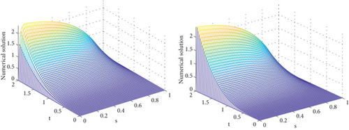
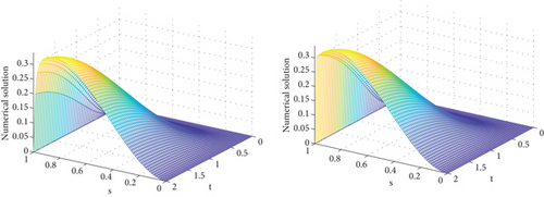
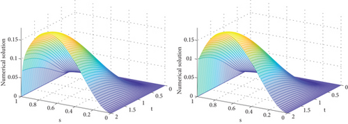
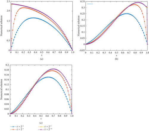
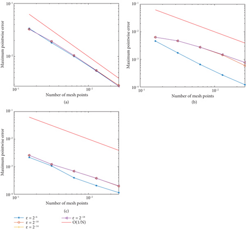
The numerical solutions of the developed method for each example are revealed in Figures 1-3. From Figure 1, we verify that a strong boundary layer is maintained along s = 0 as ε⟶0. Moreover, Figures 2 and 3 have revealed that a strong boundary layer is maintained along s = 1 as ε⟶0. Further, to show the effect of ε on the steepness of the boundary layer, the solutions are depicted in Figure 4. In each figure, we observe that as ε⟶0, the width of the boundary layer decreases, which confirms the desired result, that is, the boundary layer width of O(ε). In addition, in Figure 5, the of the method is plotted by the log–log scale. From these figures, one can see that the decreases as the step size decreases for every value of ε, which confirms the ε-uniform convergence of the developed method. The comparison of the findings of the proposed scheme with the existing recently published works is revealed in Tables 4–6. As we have seen in Table 4, the results obtained in this paper have better accuracy than those of [18, 21]. In addition, in Tables 5 and 6, it is shown that the obtained results are more accurate compared to that of [21].

Details are in the caption following the image — **Figure 1**
Open in figure viewer PowerPoint

Numerical solution of Example 1 for ε = 2⁻⁶ and ε = 2⁻²⁰, respectively.

Table 4. E^N,M and r^N,M for Example 1 and results in [18, 21].

Schemes ↓	16	32	64	128	256
	Number of intervals *N = M*
Proposed scheme
E^N,M	3.3768e − 02	1.9397e − 02	1.0778e − 02	5.4740e − 03	2.8614e − 03
r^N,M	0.7998	0.8477	0.9774	0.9359	—
Results in [18]
E^N,M	3.7225e − 02	2.1953e − 02	1.1908e − 02	6.1994e − 03	3.1627e − 03
r^N,M	0.76185	0.88249	0.94173	0.97097	—
Results in [21]
E^N,M	8.3951e − 02	4.9224e − 02	2.6666e − 02	1.3880e − 02	7.0816e − 03
r^N,M	0.77019	0.88436	0.94199	0.97086	—

Table 5. E^N,M and r^N,M for Example 2 and results in [21].

Schemes ↓	16	32	64	128	256
	Number of intervals *N = M*
Proposed scheme
E^N,M	6.3462e − 03	4.6922e − 03	2.7628e − 03	1.4893e − 03	7.7197e − 04
r^N,M	0.4356	0.7641	0.8915	0.9480	—
Results in [21]
E^N,M	1.1160e − 02	6.3269e − 03	3.3518e − 03	1.7230e − 03	8.7325e − 04
r^N,M	0.81877	0.91656	0.96001	0.97086	—

Table 6. E^N,M and r^N,M for Example 3 and results in [21].

Schemes ↓	16	32	64	128	256
	Number of intervals *N = M*
Proposed scheme
E^N,M	2.5922e − 03	1.2179e − 03	6.9552e − 04	3.8111e − 04	2.0016e − 04
r^N,M	1.0898	0.8082	0.8679	0.9291	—
Results in [21]
E^N,M	5.6185e − 03	2.9471e − 03	1.4861e − 03	7.4255e − 04	3.7060e − 04
r^N,M	0.9308	0.98776	1.0010	1.0026	—

5. Conclusion

A fitted tension spline numerical scheme is constructed to solve a SPPP with a time delay. The proposed method considered the SPPP to exhibit a parabolic boundary layer in the neighborhood of the left or right side of the domain as ε approaches 0. The solution varies abruptly in the layer region due to the presence of the perturbation parameter. The problem behaves in a multiscale character where the solution has a rapid change in the boundary layer region and is uniform otherwise. Due to this, classical numerical methods on a uniform mesh lead to an oscillatory solution and thus fail to give satisfactory results. To overcome this drawback, we proposed a fitted spline numerical method. The method comprises the backward Euler in the temporal direction and the fitted spline method in the spatial direction on uniform meshes. The developed scheme gives an accuracy of first-order both in space and time direction. Three numerical examples are considered to validate the efficiency and applicability of the proposed scheme, and the results support our theoretical findings. Concisely, the presented scheme is stable, ε-uniform, and provides more accurate numerical results compared to those of others.

Conflicts of Interest

The authors declare no conflicts of interest.

Funding

The authors received no specific funding for this work.

Open Research

Data Availability Statement

All the generated data was used. No additional data were used to support the findings of this research work from other sources.

References

1 Das A. and Natesan S., Uniformly convergent hybrid numerical scheme for singularly perturbed delay parabolic convection-diffusion problems on Shishkin mesh, Applied Mathematics and Computation. (2015) 271, 168–186, https://doi.org/10.1016/j.amc.2015.08.137, 2-s2.0-84942508971.
10.1016/j.amc.2015.08.137
Web of Science® Google Scholar
2 Ewing R. E., The Mathematics of Reservoir Simulation, 1983, SIAM, Philadelphia.
10.1137/1.9781611971071
Google Scholar
3 Baumert H., Braun P., Glos E., Müller W.-D., and Stoyan G., Modelling and computation of water quality problems in river networks, Lecture Notes in Control and Information Sciences, 1981, Springer-Velag, Berlin.
Google Scholar
4 Ansari A. R., Bakr S. A., and Shishkin G. I., A parameter-robust finite difference method for singularly perturbed delay parabolic partial differential equations, Journal of Computational and Applied Mathematics. (2007) 205, no. 1, 552–566, https://doi.org/10.1016/j.cam.2006.05.032, 2-s2.0-34247535463.
10.1016/j.cam.2006.05.032
Web of Science® Google Scholar
5 Baker C. T. H., Bocharov G. A., and Rihan F. A., A report on the use of delay differential equations in numerical modelling in the biosciences, 1999, Citeseer.
Google Scholar
6 Wang P. K. C., Asymptotic stability of a time-delayed diffusion system, Journal of Applied Mechanics. (1963) 30, no. 4, 500–504, https://doi.org/10.1115/1.3636609, 2-s2.0-85015580203.
10.1115/1.3636609
Google Scholar
7 Kumar D. and Kumari P., A parameter-uniform numerical scheme for the parabolic singularly perturbed initial boundary value problems with large time delay, Journal of Applied Mathematics and Computing. (2019) 59, no. 1-2, 179–206, https://doi.org/10.1007/s12190-018-1174-z, 2-s2.0-85041893391.
10.1007/s12190-018-1174-z
Web of Science® Google Scholar
8 Ejere A. H., Duressa G. F., Woldaregay M. M., and Dinka T. G., A robust numerical scheme for singularly perturbed differential equations with spatio-temporal delays, Frontiers in Applied Mathematics and Statistics. (2023) 9, article 1125347, https://doi.org/10.3389/fams.2023.1125347.
10.3389/fams.2023.1125347
Google Scholar
9 Tesfaye S. K., Duressa G. F., Woldaregay M. M., and Dinka T. G., Fitted computational method for singularly perturbed convection-diffusion equation with time delay, Frontiers in Applied Mathematics and Statistics. (2023) 9, article 1244490, https://doi.org/10.3389/fams.2023.1244490.
10.3389/fams.2023.1244490
Google Scholar
10 Ayele M. A., Tiruneh A. A., and Derese G. A., Hybrid fitted numerical scheme for singularly perturbed convection-diffusion problem with a small time lag, Abstract and Applied Analysis. (2023) 2023, 15, 4382780, https://doi.org/10.1155/2023/4382780.
10.1155/2023/4382780
Google Scholar
11 Govindarao L. and Mohapatra J., A second order numerical method for singularly perturbed delay parabolic partial differential equation, Engineering Computations. (2019) 36, no. 2, 420–444, https://doi.org/10.1108/EC-08-2018-0337, 2-s2.0-85058347474.
10.1108/EC-08-2018-0337
Web of Science® Google Scholar
12 Gowrisankar S. and Natesan S., ε-Uniformly convergent numerical scheme for singularly perturbed delay parabolic partial differential equations, International Journal of Computer Mathematics. (2017) 94, no. 5, 902–921, https://doi.org/10.1080/00207160.2016.1154948, 2-s2.0-84961889779.
10.1080/00207160.2016.1154948
Web of Science® Google Scholar
13 Salama A. and Al-Amery D. G., A higher order uniformly convergent method for singularly perturbed delay parabolic partial differential equations, International Journal of Computer Mathematics. (2017) 94, no. 12, 2520–2546, https://doi.org/10.1080/00207160.2017.1284317, 2-s2.0-85012297089.
10.1080/00207160.2017.1284317
Web of Science® Google Scholar
14 Podila P. C. and Kumar K., A new stable finite difference scheme and its convergence for time-delayed singularly perturbed parabolic PDES, Computational and Applied Mathematics. (2020) 39, no. 3, 1–16, https://doi.org/10.1007/s40314-020-01170-2.
10.1007/s40314-020-01170-2
Web of Science® Google Scholar
15 Das A. and Natesan S., Second-order uniformly convergent numerical method for singularly perturbed delay parabolic partial differential equations, International Journal of Computer Mathematics. (2018) 95, no. 3, 490–510, https://doi.org/10.1080/00207160.2017.1290439, 2-s2.0-85014557906.
10.1080/00207160.2017.1290439
Web of Science® Google Scholar
16 Kumar K., Gupta T., Chakravarthy P. P., and Rao R. N., An adaptive mesh selection strategy for solving singularly perturbed parabolic partial differential equations with a small delay, Applied Mathematics and Scientific Computing, 2019, Birkhäuser, 67–76, https://doi.org/10.1007/978-3-030-01123-9_8, 2-s2.0-85061330678.
10.1007/978-3-030-01123-9_8
Google Scholar
17 Kumar K., Podila P. C., Das P., and Ramos H., A graded mesh refinement approach for boundary layer originated singularly perturbed time-delayed parabolic convection diffusion problems, Mathematicsl Methods in the Applied Sciences. (2021) 44, no. 16, 12332–12350, https://doi.org/10.1002/mma.7358.
10.1002/mma.7358
Web of Science® Google Scholar
18 Tesfaye S. K., Woldaregay M. M., Dinka T. G., and Duressa G. F., Fitted computational method for solving singularly perturbed small time lag problem, BMC Research Notes. (2022) 15, no. 1, https://doi.org/10.1186/s13104-022-06202-0, 36221103.
10.1186/s13104-022-06202-0
PubMed Web of Science® Google Scholar
19 Babu G. and Bansal K., A high order robust numerical scheme for singularly perturbed delay parabolic convection-diffusion problems, Journal of Applied Mathematics and Computing. (2022) 68, no. 1, 363–389, https://doi.org/10.1007/s12190-021-01512-1.
10.1007/s12190-021-01512-1
Web of Science® Google Scholar
20 Negero N. T. and Duressa G. F., A method of line with improved accuracy for singularly perturbed parabolic convection-diffusion problems with large temporal lag, Results in Applied Mathematics. (2021) 11, article 100174, https://doi.org/10.1016/j.rinam.2021.100174.
10.1016/j.rinam.2021.100174
Google Scholar
21 Negero N. T. and Duressa G. F., Uniform convergent solution of singularly perturbed parabolic differential equations with general temporal-lag, Iranian Journal of Science and Technology, Transactions A: Science. (2022) 46, no. 2, 507–524, https://doi.org/10.1007/s40995-021-01258-2.
10.1007/s40995-021-01258-2
Web of Science® Google Scholar
22 Daba I. T. and Duressa G. F., A novel algorithm for singularly perturbed parabolic differential-difference equations, Research in Mathematics. (2022) 9, no. 1, article 2133211, https://doi.org/10.1080/27684830.2022.2133211.
10.1080/27684830.2022.2133211
Google Scholar
23 Shishkin G. I. and Shishkina L. P., Difference Methods for Singularly Perturbed Problems, 2008, CRC.
10.1201/9780203492413
Google Scholar
24 Protter M. and Weinberger H., Maximum Principles in Differential Equations, 1967, Prentice-Hall Inc., Englewood Cliffs, New Jersey.
Web of Science® Google Scholar
25 Tian H., Numerical treatment of singularly perturbed delay differential equations, 2000, Ph. D. thesis, University of Manchester.
Google Scholar
26 Clavero C., Jorge J. C., and Lisbona F., A uniformly convergent scheme on a nonuniform mesh for convection-diffusion parabolic problems, Computational and Applied Mathematics. (2003) 154, no. 2, 415–429, https://doi.org/10.1016/S0377-0427(02)00861-0, 2-s2.0-0037849987.
10.1016/S0377-0427(02)00861-0
Web of Science® Google Scholar
27 Kellogg R. B. and Tsan A., Analysis of some difference approximations for a singular perturbation problem without turning points, Mathematics of Computation. (1978) 32, no. 144, 1025–1039, https://doi.org/10.1090/S0025-5718-1978-0483484-9, 2-s2.0-84966216257.
10.1090/S0025-5718-1978-0483484-9
Web of Science® Google Scholar
28 Khan I. and Aziz T., Tension spline method for second-order singularly perturbed boundary-value problems, International Journal of Computer Mathematics. (2005) 82, no. 12, 1547–1553, https://doi.org/10.1080/00207160410001684280, 2-s2.0-30844469072.
10.1080/00207160410001684280
Web of Science® Google Scholar
29 O’Malley R. E., Singular Perturbation Methods for Ordinary Differential Equations, 1991, Springer.
10.1007/978-1-4612-0977-5
Google Scholar
30 Woldaregay M. M., Aniley W. T., and Duressa G. F., Novel numerical scheme for singularly perturbed time delay convection-diffusion equation, Advances in Mathematical Physics. (2021) 2021, 13, 6641236, https://doi.org/10.1155/2021/6641236.
10.1155/2021/6641236
Web of Science® Google Scholar

Citing Literature

All articles

Fitted Tension Spline Scheme for a Singularly Perturbed Parabolic Problem With Time Delay

Abstract

1. Introduction

2. Continuous Problem

2.1. A Priori Bounds

3. Numerical Method

3.1. The Time Semidiscretization

3.2. The Spatial Discretization

3.2.1. Description of the Method

3.2.2. Exponential Fitting Factor

3.3. Convergence Analysis

4. Numerical Results

5. Conclusion

Conflicts of Interest

Funding

Open Research

Data Availability Statement

References

Citing Literature

Figures

References

Information

About Wiley Online Library

Help & Support

Opportunities

Connect with Wiley

Fitted Tension Spline Scheme for a Singularly Perturbed Parabolic Problem With Time Delay

Abstract

1. Introduction

2. Continuous Problem

2.1. A Priori Bounds

3. Numerical Method

3.1. The Time Semidiscretization

3.2. The Spatial Discretization

3.2.1. Description of the Method

3.2.2. Exponential Fitting Factor

3.3. Convergence Analysis

4. Numerical Results

5. Conclusion

Conflicts of Interest

Funding

Open Research

Data Availability Statement

References

Citing Literature

Figures

References

Related

Information