This paper examines the dynamic behavior of a particular category of discrete predator-prey system that feature both fear effect and refuge, using both analytical and numerical methods. The critical coefficients and properties of bifurcating periodic solutions for Flip and Hopf bifurcations are computed using the center manifold theorem and bifurcation theory. Additionally, numerical simulations are employed to illustrate the bifurcation phenomenon and chaos characteristics. The results demonstrate that period-doubling and Hopf bifurcations are two typical routes to generate chaos, as evidenced by the calculation of the maximum Lyapunov exponents near the critical bifurcation points. Finally, a feedback control method is suggested, utilizing feedback of system states and perturbation of feedback parameters, to efficiently manage the bifurcations and chaotic attractors of the discrete predator-prey model.

1. Introduction

In exploring population dynamics, continuum modelling is often used to explain population trends in situations where populations are large or where there are overlapping generations [1, 2]. However, when there is no overlap between generations of a population, the growth pattern of the population will show obvious stages and discontinuities. In this case, a discrete model can more accurately capture and reflect this discontinuity in population change. Discrete predator-prey systems can exhibit complex dynamical behavior, which has attracted many researchers to study them [3–6]. Zhang et al. [7] studied the dynamics of a discrete FitzHugh–Nagumo model by applying central manifold and normal form analysis and demonstrated that the system is capable of undergoing Neimark–Sacker and flip bifurcations even in the absence of diffusion. Li et al. [8] obtained rich dynamic properties by building a space-time discrete model with periodic boundary conditions. Therefore, discrete dynamical systems can have more complex dynamics, and their dynamic behavior can more closely approximate the complex dynamics of the phenomena represented by the model.

Since the biological population itself is a complex nonlinear system, this nonlinearity is the fundamental cause of the occurrence of chaos [9, 10]. Through the study of biological groups, we can see that there are many chaotic behaviors embedded in them [11]. Such chaotic phenomena are not limited to animal reproduction and evolution, such as competition and parasitism between the groups [12]. However, chaos in biological groups is not all good, and the negative chaotic situations that exist in nature can have a negative effect on human survival and development; therefore, controlling these chaotic situations is important for maintaining the stability of the ecosystem [13–17]. Discrete systems have two special bifurcations, flip bifurcation and Hopf bifurcation, which in turn are the two ways for discrete systems to move towards chaos. There are now many ways of controlling the chaos generated by the model: Vinoth et al. [18] describe three different approaches to chaos control: state feedback, pole placement, and hybrid control. Nowadays, nature, because of prolonged disturbances, has destroyed its natural rules of reproduction and put it on the verge of extinction, so it is important to carry out the study of chaos control of biological groups with important theoretical and practical application value.

Predator-prey interactions play a crucial role in the study of biological systems and population dynamics. Various examples have been explored, including populations with different functional response functions [19–24]. Additionally, the impact of having a refuge on population dynamics has been examined [25–28]. The reproductive capacity of prey populations is a vital factor in understanding population dynamics. The size of the prey population is influenced by the number of predators, which, in turn, is affected by the size of the prey population. Furthermore, the fear of predators among prey species significantly impacts the reproductive capacity of prey populations, thereby influencing the entire predation system. Wang et al. [29] proposed an expression f(K, y) = (1/1 + Ky) to describe the effect of fear on prey populations, where the degree of fear is represented by K. This expression can be utilized to predict the size of the prey population, which ultimately affects the stability of the entire ecosystem. Fakhry et al. [30] proposed a square root prey-predator model with fear

(1)

with initial condition x(t) > 0 and y(t) > 0, where K indicates the level of fear, α indicates the death rate of the predator in the absence of prey, β indicates the conversion rate of prey to predator, and r is the growth rate of the prey.

In 2019, Zhang et al. [31] investigated predator-prey systems with fear effects and refuge

(2)

where K indicates the level of fear, α indicates the endowment growth rate of the bait, and r indicates the predator mortality rate. (β/a) indicates the maximum amount of predators eaten by each predator per unit of time, b indicates the coefficient of competition within the prey population, c indicates the conversion factor, and (1 − m)x indicates the amount of prey taken, m ∈ [0, 1). The effects of fear and the impact of refuges on system stability are discussed. This model can better describe dynamic behaviors such as interactions and competition between species in ecosystems.

The discrete form of (2) can be obtained using Euler’s method as follows:

(3)

This paper focuses on analyzing the model bifurcation and chaotic properties. In the first part, the existence and stability of the equilibrium point are discussed. In the second and third parts, the conditions for the existence of flip and Hopf bifurcation at the positive equilibrium point are considered, and the direction of the flip and Hopf bifurcation at the positive equilibrium point is derived by using the central manifold theorem. In the fourth part, the maximum Lyapunov exponent is used to discuss the occurrence of chaotic situations inside the system and to control the resulting chaotic situations, and finally, numerical simulations verify the correctness of the theoretical proofs.

2. Existence and Stability of Equilibrium Points

It is evident that system (3) possesses a trivial equilibrium point N₀(0, 0) and a boundary equilibrium point N₁(α/b, 0).

Assuming (H₁) : cβ − ar > 0

If (H₁) holds, the only positive equilibrium point of the system can be obtained as N^∗(x^∗, y^∗), where x^∗ = r/(cβ − ar)(1 − m), , .

The Jacobi matrix

of system (3) at any equilibrium point is given by

(4)

To investigate the stability analysis of the equilibrium point of system (3), we present the following lemma. By utilizing the connections between the coefficients and roots of a quadratic equation [32], one can readily derive the following results.

Lemma 1. Assume that F(λ) = λ² − Aλ + B and F(1) > 0 with λ₁, λ₂ are roots of F(λ) = 0. Then, the following results hold true:

(i)
|λ₁| < 1 and |λ₂| < 1 if and only if F(−1) > 0, B < 1.
(ii)
|λ₁| < 1 and |λ₂| > 1, or |λ₁| > 1 and |λ₂| < 1 if and only if F(−1) < 0.
(iii)
|λ₁| > 1 and |λ₂| > 1 if and only if F(−1) < 0, B > 1.
(iv)
λ₁ and λ₂ are complex and |λ₁| = 1, |λ₂| = 1 if and only if A² − 4B < 0 and B = 1.

Theorem 2. For the trivial equilibrium point N₀(0, 0), the characteristic equation of system (3) at N₀(0, 0) has two eigenvalues, λ₁ = 1 + hα and λ₂ = 1 − hr

(i)
If h < 2/r, then |λ₁| > 1, |λ₂| < 1, N₀(0, 0) is a saddle point.
(ii)
If h > 2/r, then |λ₁| > 1, |λ₂| > 1, N₀(0, 0) is a source.

Theorem 3. For the boundary equilibrium point N₁(α/b, 0), the characteristic equation of system (3) at N₁(α/b, 0) has the eigenvalue λ₁ = 1 − hα, λ₂ = 1 + h(−r + cβ(1 − m)α/b + a(1 − m)α), let l = (cβ − aα)(1 − m)

(i)
If , then |λ₁| < 1, |λ₂| < 1, N₁(α/b, 0) is a sink.
(ii)
If , then |λ₁| > 1, |λ₂| < 1, or if , then |λ₁| < 1, |λ₂| > 1, N₁(α/b, 0) is a saddle point.
(iii)
If or , then |λ₁| > 1, |λ₂| > 1, N₁(α/b, 0) is a source.

For the point N^∗(x^∗, y^∗), we have

(5)

Furthermore, the characteristic polynomial of

when evaluated at the equilibrium point N^∗(x^∗, y^∗) can be expressed as follows:

(6)

where

Theorem 4. For the point N^∗(x^∗, y^∗)

(i)
If , then |λ₁| < 1, |λ₂| < 1, N^∗(x^∗, y^∗) is a sink.
(ii)
If , then |λ₁| < 1 and |λ₂| > 1, or |λ₁| > 1 and |λ₂| < 1, N^∗(x^∗, y^∗) is a saddle point.
(iii)
If , then |λ₁| > 1 and |λ₂| > 1, N^∗(x^∗, y^∗) is a source.
(iv)
If , then λ₁, λ₂ is a pair of conjugate complex roots.

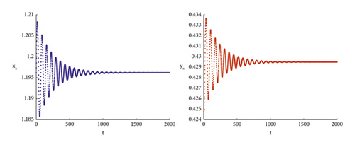
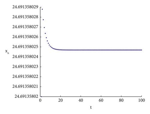
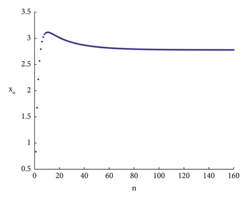
To validate the accuracy of the theoretical proof, numerical simulations are conducted in the following sections. When the parameters are taken as h = 0.1, c = 0.9, r = 0.1, b = 0.01, d = 0.82146, e = 0.9, a = 0.5, K = 34.555, m = 0.89, Theorem 4 of (i) is satisfied, see Figure 1.

Details are in the caption following the image — **Figure 1**
Open in figure viewer PowerPoint

Equilibrium solution at N^∗(x^∗, y^∗) ≈ (1.19617, 0.4247) when the parameters are taken as h = 0.1, c = 0.9, r = 0.1, b = 0.01, d = 0.82146, e = 0.9, a = 0.5, K = 34.555, and m = 0.89.

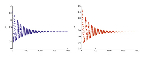
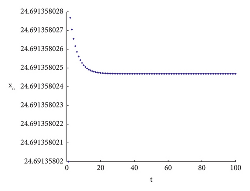
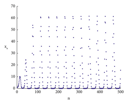
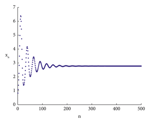
With other parameters are kept constant, let K = 15, through the image can be obtained when the degree of fear is different, the final stability of the system is different, see Figure 2.

3. Flip Bifurcation at Positive Equilibrium Point

3.1. Conditions for the Existence of Flip Bifurcation

To obtain the bifurcation parameters, consider the transformations

, system (3) can be approximated as

(7)

Using the Taylor expansion at the point x^∗, y^∗ yields the following expression:

(8)

where

, u₄ = 0,

According to the characteristic polynomial (6), we can get

(9)

Since the step size h > 0, it is possible to obtain the branching value . Here,

Let h = h^∗ + δ. We consider δ as a small bifurcation parameter, and the perturbation of system (7) can be described by the following system, where |δ| ≪ 1.

(10)

where L = ((2αl²/i₂) − (2br/l) − (β(1 − m)i₁/i₃)),

, and i₃ = 2K(l + α(1 − m)r)².

In this case the characteristic polynomial (7) can be rewritten as

(11)

solve for

(12)

The transversal condition at N^∗(x^∗, y^∗) is

(13)

If , flip bifurcation occurs at the positive equilibrium point N^∗(x^∗, y^∗).

3.2. The Normal Form of Flip Bifurcation Solutions

Define

(14)

If the eigenvalue of A is λ = −1, then the corresponding eigenvector is

(15)

If the eigenvalue of A is λ = λ₂, then the corresponding eigenvector is

(16)

Then the following invertible matrix can be obtained:

(17)

Using the transformation

, system (7) is transformed into

(18)

where

(19)

Using the transformation

, system (10) becomes

(20)

let

(21)

then

(22)

During our analysis, we will utilize the central manifold theorem and normal form theory to investigate the direction of the flip bifurcation at the point N^∗(x^∗, y^∗).

Let

(23)

where the coefficients of θ₁ and θ₂ are derived from (20).

Theorem 5. The system exhibits a flip bifurcation at the immobile point N^∗(x^∗, y^∗) if both θ₁ and θ₂ are nonzero, and it is stable (unstable) at that point with a period of 2 if θ₂ > 0(<0).

Proof. In a sufficiently small neighborhood with parameter δ = 0, there exists a central manifold located at (0, 0):

(24)

Substituting (24) into (20), the solution is given as

(25)

By focusing on the system of equations at W^c(0, 0), we can derive the following outcome:

(26)

which

, r₂ = d₁₁ = a₁₁k₁₁ + a₁₂k₂₁, r₃ = d₁₂m₁ + f₁₁ + e₁₂m₂, r₄ = d₁₂m₂, and r₅ = e₁₂m₁ + e₁₄.

Based on the reference [33], it is stated that when considering values at (N, P, δ) = (0, 0, 0) and having θ₁ ≠ 0, θ₂ ≠ 0, the system exhibits a flip bifurcation at the fixed point N^∗(x^∗, y^∗). If θ₂ > 0(<0), the point with a period of 2 is stable (unstable).

which

(27)

This completes the proof.

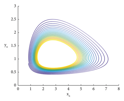
To validate the accuracy of the theoretical proof, numerical simulations are conducted in the following sections. When the parameters are taken as h = 4.05937004, r = 0.8, d = 0.5, c = 0.9, b = 0.02, e = 0.6, a = 0.6, K = 9.99, m = 0.46, (7) is satisfied; see Figure 3.

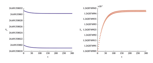
Remark 6. From an ecological perspective, the occurrence of a flip bifurcation is characterized by population size fluctuating in cycles of 2, 4, 8, and so on until a chaotic state is reached. This phenomenon implies that prey populations cannot maintain stability, ultimately resulting in an ecological imbalance.

4. Hopf Bifurcation at Positive Equilibrium Point

4.1. Existence Conditions for Hopf Bifurcation

If a Hopf bifurcation occurs near a positive equilibrium point N^∗(x^∗, y^∗), the characteristic polynomial (3) must have a pair of conjugate unit complex roots. Consequently, we can deduce the bifurcation parameter as follows:

(28)

Since the step size h > 0, the choice of the bifurcation parameter under the condition cβ − ar > 0, α > 0 and 0 ≤ m < 1 − (br/α(cβ − ar)) is given by

(29)

where

, and

Taking δ as a small bifurcation parameter, i.e.,

, |δ| ≪ 1. Then, characteristic (6) can be written as

(30)

in which

. The roots of the equation at

are

(31)

in the meantime

, (d|λ_1,2|/ dδ)|_δ=0 ≠ 0 can be obtained if and only if

If s(0) ≠ 0, 1, we have , , where n = 1, 2, 3, 4.

If , Hopf bifurcation occurs at the positive equilibrium point N^∗(x^∗, y^∗).

4.2. Normal Form of Hopf Bifurcation at Positive Equilibria

Assuming that λ₁ = u + iv, λ₂ = u − iv, where u = (1/2)(−2 + h₁L),

. The corresponding invertible matrix can be obtained as

(32)

The corresponding inverse matrix is

(33)

Using the following transformations

, (10) is converted to

(34)

in which

(35)

The coefficients are

(36)

(37)

By utilizing the central manifold theorem and the normal form theory, we can determine the bifurcation direction of the Hopf bifurcation at the positive equilibrium point. Furthermore, by applying the canonical type theory of the Hopf bifurcation, we can evaluate the equation at

(38)

Theorem 7. If s(0) ≠ 0, 1 and M ≠ 0, a Hopf bifurcation occurs at a positive equilibrium point N^∗(x^∗, y^∗). Moreover, if M < 0, an attracting invariant closed curve bifurcates from the equilibrium point for δ > 0. On the other hand, if M > 0, a repelling invariant closed curve bifurcates from the equilibrium point for δ < 0.

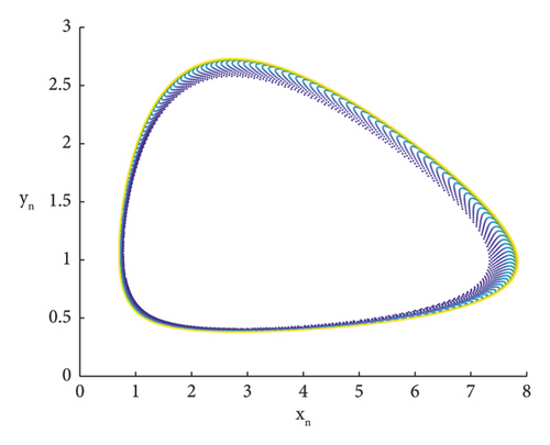
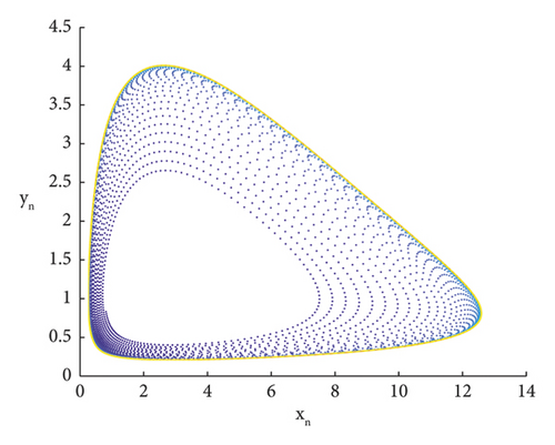
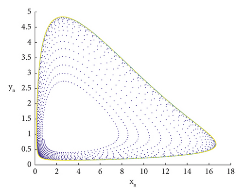
To validate the accuracy of the theoretical proof, numerical simulations are conducted in the following sections. When the parameters are taken as h = 0.168989, r = 0.2, K = 4.94, d = 0.8, c = 0.8, b = 0.01, e = 0.5, a = 0.5, m = 0.76, (7) is satisfied; see Figure 4.

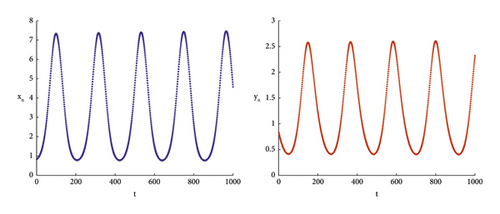
Remark 8. From an ecological perspective, as the parameter h approaches the critical value h^∗, a stable curve emerges at the equilibrium point N^∗(x^∗, y^∗), indicating a stable coexistence between the prey and predator populations. Conversely, if the constant curve at the equilibrium point N^∗(x^∗, y^∗) becomes unstable as h increases, the populations of prey and predators will fail to reach a stable state, leading to an ecological imbalance within the ecosystem.

5. Chaotic Analysis

In general, flip bifurcation and Hopf bifurcation are two ways in which discrete systems move towards chaos. Under the condition of the existence of two kinds of bifurcations, applying perturbations to the bifurcation parameters, sometimes a chaotic situation occurs, which is discussed in the following.

5.1. Existence of Chaos

Definition 9 (see [34].)For the system x_n+1 = f(x_n), y_n+1 = f(y_n), if a small perturbation is applied to the system, the system will diverge as the number of iterations increases, and the degree of divergence is usually expressed using the maximum Lyapunov index, which is given by

(39)

Theorem 10 (see [34].)If λ < 0, it is an indication that neighboring points will eventually converge to a single point. This is the equivalent of stable, motionless points and periodic motion. On the other hand, if λ > 0, it means that neighboring points will eventually separate from each other. This means that orbits are locally unstable and chaotic.

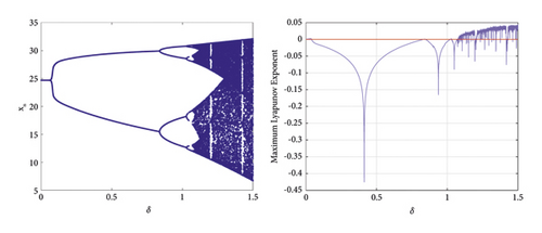
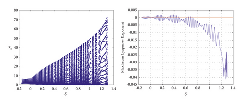
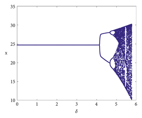
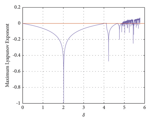
After selecting the perturbation δ = (0, 1.5), the trend of x is analyzed numerically, and through numerical simulation, the maximum Lyapunov exponential map agrees with the trend of the bifurcation map, see Figures 5-7.

5.2. Chaos Control

Using the state feedback control method [35–37] to stabilize the chaotic orbit at an unstable equilibrium point of the system (3) and to achieve this, we introduce the following controlled system, which corresponds to (3):

(40)

The feedback control is defined as U_n = σ(x_n − x^∗) + θ(y_n − y^∗), where σ and θ are the feedback gains and N^∗(x^∗, y^∗) represents the only positive equilibrium point of the system.

The Jacobi matrix of the controlled system at the exclusive positive equilibrium point is displayed underneath:

(41)

where

, J₂₂ = 1 + h(−r + (cβ(1 − m)x^∗/1 + a(1 − m)x^∗)).

From the Jacobi matrix, the corresponding characteristic equation is

(42)

Let λ₁, λ₂ be the two eigenvalues of the equation, which gives

(43)

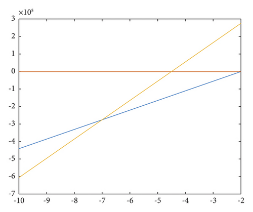
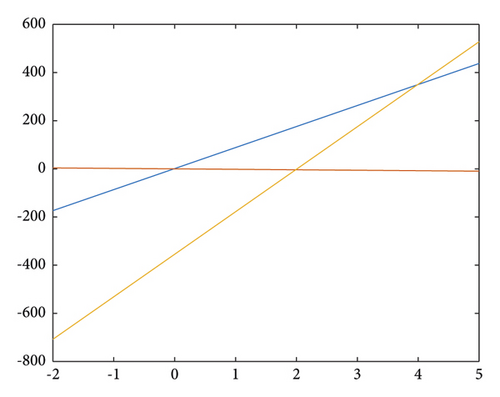
To determine the lines of marginal stability, we need to solve the equations λ₁ = ±1 and λ₁λ₂ = 1. These equations impose constraints that guarantee the absolute values of λ₁ and λ₂ are both less than 1. By finding the solutions to these equations, we can identify the boundaries of stability.

Assume that λ₁λ₂ = 1, it is possible to obtain L₁ : J₁₁J₂₂ − J₂₁J₁₂ − 1 = σJ₂₂ − θJ₂₁.

Next, assuming λ₁ = 1, one obtains L₂ : σ(1 − J₂₂) + θJ₂₁ = J₁₁ + J₂₂ − 1 − J₁₁J₂₂ + J₂₁J_12.

Assuming λ₁ = −1, one obtains L₃ : σ(1 + J₂₂) − θJ₂₁ = J₁₁ + J₂₂ + 1 + J₁₁J₂₂ − J₂₁J₁₂.

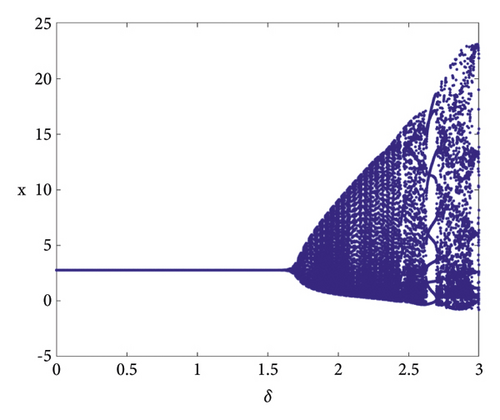
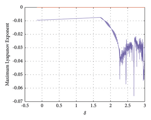
It is evident that, for specific parameter values, the stable eigenvalues are situated within the triangular region defined by the straight lines L₁, L₂, L₃; see Figures 8 and 9. By selecting the appropriate parameter values in the restricted area, it becomes apparent that the perturbation values increase significantly when chaos emerges within the controlled region;, see Figures 10 and 11. Furthermore, the temporal evolution of the population numbers, both before and after implementing control measures, can be effectively validated through visual representations; see Figures 12 and 13.

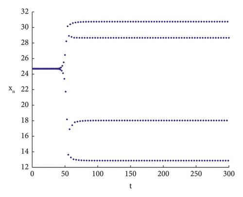
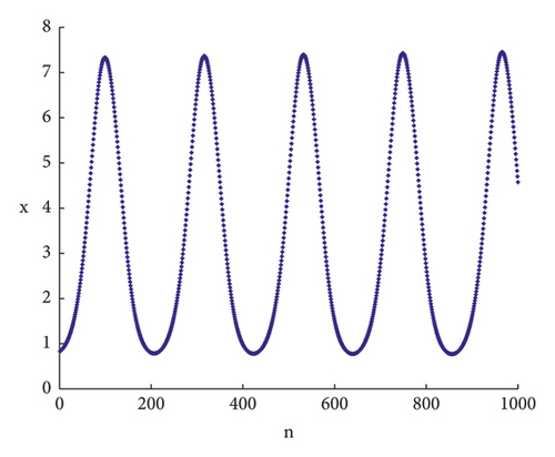
Remark 11. From the ecological point of view, when unfavourable chaos occurs, the antidisturbance ability of the ecosystem is greatly enhanced by carrying out chaos control, which is conducive to maintaining the stability of the ecosystem and reducing the problem of ecological imbalance. As an example, greening and the establishment of biological shelters can effectively reduce the state of chaos among groups of organisms, thus effectively protecting and managing the diversity of species.

6. Conclusion

In this paper, we investigate a discrete predator-prey model incorporating fear effects and refuge. We begin by discussing the local stability and instability conditions of the three equilibrium points of system (3). Specifically, we analyze the occurrence of flip bifurcation at eigenvalues |λ₁| = −1 and |λ₂| < 1 of characteristic (6). Additionally, we explore the Hopf bifurcation that arises when the eigenvalues of characteristic (6) form a pair of conjugate unit complex roots. We also examine the bifurcation directions associated with these two types of bifurcations.

The chaotic behavior of the system is investigated through both theoretical proofs and numerical simulations. We demonstrate that chaotic dynamics can be controlled using the feedback control method. Bifurcation diagrams and maximum Lyapunov exponent diagrams clearly illustrate the significant increase in perturbation values when system (3) exhibits chaos after control.

From a biological perspective, the stability analysis of the equilibrium points reveals that, under the influence of fear and other factors, the predator and prey populations eventually reach an equilibrium state, allowing for harmonious coexistence. By controlling the chaotic situations arising from flip and Hopf bifurcations, we can effectively suppress chaotic behavior among organisms. This can be achieved through various human-imposed interventions such as greening, establishing biological refuges, and implementing other measures. These interventions are beneficial for the survival and development of biological populations.

In future research, it would be worthwhile to explore different chaos control methods in order to achieve improved control effects.

Conflicts of Interest

The authors declare that they have no conflicts of interest.

Authors’ Contributions

The idea of this research was introduced by W. Li. All the authors contributed to the main results and numerical simulations. C. Zhang and M Wang contributed to revising the manuscript.

Acknowledgments

This research was supported by the Fundamental Research Funds for the Central Universities (no. 60201523050).

Open Research

Data Availability

No data were used to support the findings of this study.

References

1 Wang J., Cai Y., Fu S., and Wang W., The effect of the fear factor on the dynamics of a predator-prey model incorporating the prey refuge, Chaos. (2019) 29, no. 8, 83109, https://doi.org/10.1063/1.5111121, 2-s2.0-85070704018.
10.1063/1.5111121
PubMed Web of Science® Google Scholar
2 Aziz-Alaoui M. A. and Daher Okiye M., Boundedness and global stability for a predator-prey model with modified Leslie-Gower and Holling-type II schemes, Applied Mathematics Letters. (2003) 16, no. 7, 1069–1075, https://doi.org/10.1016/s0893-9659(03)90096-6, 2-s2.0-0242364789.
10.1016/S0893-9659(03)90096-6
Web of Science® Google Scholar
3 Li S. and Zhang W., Bifurcations of a discrete prey-predator model with Holling type II functional response, Discrete & Continuous Dynamical Systems- B. (2010) 14, no. 1, 159–176, https://doi.org/10.3934/dcdsb.2010.14.159, 2-s2.0-77957794727.
10.3934/dcdsb.2010.14.159
Web of Science® Google Scholar
4 Hone A. N. W., Irle M. V., and Thurura G. W., On the Neimark-Sacker bifurcation in a discrete predator-prey system, Journal of Biological Dynamics. (2010) 4, no. 6, 594–606, https://doi.org/10.1080/17513750903528192, 2-s2.0-79960480422.
10.1080/17513750903528192
CAS PubMed Google Scholar
5 Rodrigues L. A. D., Mistro D. C., and Petrovskii S., Pattern formation, long-term transients, and the Turing-Hopf bifurcation in a space-and time-discrete predator-prey system, Bulletin of Mathematical Biology. (2011) 73, no. 8, 1812–1840, https://doi.org/10.1007/s11538-010-9593-5, 2-s2.0-79959574497.
10.1007/s11538-010-9593-5
PubMed Web of Science® Google Scholar
6 Petrovskii S. V., Morozov A. Y., and Venturino E., Allee effect makes possible patchy invasion in a predator-prey system, Ecology Letters. (2002) 5, no. 3, 345–352, https://doi.org/10.1046/j.1461-0248.2002.00324.x, 2-s2.0-0036113356.
10.1046/j.1461-0248.2002.00324.x
Web of Science® Google Scholar
7 Zhang X., Zhang C., and Zhang Y., Pattern dynamics analysis of a time-space discrete FitzHugh-Nagumo(FHN) model based on coupled map lattices, Computers and Mathematics with Applications&Mathematics with Applications. (2024) 157, 92–123, https://doi.org/10.1016/j.camwa.2023.12.030.
10.1016/j.camwa.2023.12.030
Web of Science® Google Scholar
8 Li T., Zhang X., and Zhang C., Pattern dynamics analysis of a space-time discrete spruce budworm model, Chaos, Solitons and Fractals. (2024) 179, 114423, https://doi.org/10.1016/j.chaos.2023.114423.
10.1016/j.chaos.2023.114423
Web of Science® Google Scholar
9 Ivancevic V. G., Ivancevic T. T., Liang Z., He S., Wang H., and Sun K., Complex nonlinearity: chaos, phase transitions, topology change and path integrals, The European Physical Journal Plus. (2022) 137, no. 3.
Google Scholar
10 Bertuglia C. S. and Vaio F., Nonlinearity, Chaos, and Complexity: The Dynamics of Natural and Social Systems, 2005, Oxford University Press, Oxford, UK.
10.1093/oso/9780198567905.001.0001
Google Scholar
11 Lei C., Han X., and Wang W., Bifurcation analysis and chaos control of a discrete-time prey-predator model with fear factor, Mathematical Biosciences and Engineering. (2022) 19, no. 7, 6659–6679, https://doi.org/10.3934/mbe.2022313.
10.3934/mbe.2022313
PubMed Web of Science® Google Scholar
12 Luo X. S., Chen G., Hong Wang B., and Qing Fang J., Hybrid control of period-doubling bifurcation and chaos in discrete nonlinear dynamical systems, Chaos, Solitons and Fractals. (2003) 18, no. 4, 775–783, https://doi.org/10.1016/s0960-0779(03)00028-6, 2-s2.0-0038239703.
10.1016/S0960-0779(03)00028-6
Web of Science® Google Scholar
13 Singh A. and Sharma V. S., Bifurcations and chaos control in a discrete-time prey-predator model with Holling type-II functional response and prey refuge, Journal of Computational and Applied Mathematics. (2023) 418, https://doi.org/10.1016/j.cam.2022.114666, 114666.
10.1016/j.cam.2022.114666
Web of Science® Google Scholar
14 Akhtar S., Ahmed R., Batool M., Shah N. A., and Chung J. D., Stability, bifurcation and chaos control of a discretized Leslie prey-predator model, Chaos, Solitons and Fractals. (2021) 152, 111345, https://doi.org/10.1016/j.chaos.2021.111345.
10.1016/j.chaos.2021.111345
Web of Science® Google Scholar
15 Salman S. M., Yousef A. M., and Elsadany A. A., Stability, bifurcation analysis and chaos control of a discrete predator-prey system with square root functional response, Chaos, Solitons and Fractals. (2016) 93, 20–31, https://doi.org/10.1016/j.chaos.2016.09.020, 2-s2.0-84991240540.
10.1016/j.chaos.2016.09.020
Web of Science® Google Scholar
16 Hastings A. and Powell T., Chaos in a three-species food chain, Ecology. (1991) 72, no. 3, 896–903, https://doi.org/10.2307/1940591, 2-s2.0-0025956240.
10.2307/1940591
Web of Science® Google Scholar
17 May R. M., Biological populations with nonoverlapping generations: stable points, stable cycles, and chaos, Science. (1974) 186, no. 4164, 645–647, https://doi.org/10.1126/science.186.4164.645, 2-s2.0-0016394337.
10.1126/science.186.4164.645
CAS PubMed Web of Science® Google Scholar
18 Vinoth S., Sivasamy R., and Sathiyanathan K., A novel discrete-time Leslie-Gower model with the impact of Allee effect in predator population, Complexity. (2022) .
10.1155/2022/6931354
Web of Science® Google Scholar
19 Arsie A., Kottegoda C., and Shan C., A predator-prey system with generalized Holling type IV functional response and Allee effects in prey, Journal of Differential Equations. (2022) 309, 704–740, https://doi.org/10.1016/j.jde.2021.11.041.
10.1016/j.jde.2021.11.041
Web of Science® Google Scholar
20 Vinoth S., Sivasamy R., Sathiyanathan K., Unyong B., Rajchakit G., Vadivel R., and Gunasekaran N., The dynamics of a Leslie type predator-prey model with fear and Allee effect, Advances in Difference Equations. (2021) 2021, 338–422, https://doi.org/10.1186/s13662-021-03490-x.
10.1186/s13662-021-03490-x
Web of Science® Google Scholar
21 Jamil A. R. M. and Naji R. K., Modeling and analysis of the influence of fear on the Harvested modified Leslie-Gower model Involving nonlinear prey refuge, Mathematics. (2022) 10, no. 16, https://doi.org/10.3390/math10162857.
10.3390/math10162857
Web of Science® Google Scholar
22 Kazarinoff N. D. and Van Den Driessche P., A model predator-prey system with functional response, Mathematical Biosciences. (1978) 39, no. 1-2, 125–134, https://doi.org/10.1016/0025-5564(78)90031-7, 2-s2.0-0018098741.
10.1016/0025-5564(78)90031-7
Web of Science® Google Scholar
23 Wang J., Shi J., and Wei J., Predator-prey system with strong Allee effect in prey, Journal of Mathematical Biology. (2011) 62, no. 3, 291–331, https://doi.org/10.1007/s00285-010-0332-1, 2-s2.0-79951508642.
10.1007/s00285-010-0332-1
PubMed Web of Science® Google Scholar
24 Auger P., Mchich R., Chowdhury T., Sallet G., Tchuente M., and Chattopadhyay J., Effects of a disease affecting a predator on the dynamics of a predator-prey system, Journal of Theoretical Biology. (2009) 258, no. 3, 344–351, https://doi.org/10.1016/j.jtbi.2008.10.030, 2-s2.0-67349119470.
10.1016/j.jtbi.2008.10.030
PubMed Web of Science® Google Scholar
25 Cressman R. and Garay J., A predator-prey refuge system: evolutionary stability in ecological systems, Theoretical Population Biology. (2009) 76, no. 4, 248–257, https://doi.org/10.1016/j.tpb.2009.08.005, 2-s2.0-70449130484.
10.1016/j.tpb.2009.08.005
PubMed Web of Science® Google Scholar
26 Ma Z., Li W., Zhao Y., Wang W., Zhang H., and Li Z., Effects of prey refuges on a predator-prey model with a class of functional responses: the role of refuges, Mathematical Biosciences. (2009) 218, no. 2, 73–79, https://doi.org/10.1016/j.mbs.2008.12.008, 2-s2.0-62249093792.
10.1016/j.mbs.2008.12.008
PubMed Web of Science® Google Scholar
27 Berezovskaya F. S., Song B., and Castillo-Chavez C., Role of prey dispersal and refuges on predator-prey dynamics, SIAM Journal on Applied Mathematics. (2010) 70, no. 6, 1821–1839, https://doi.org/10.1137/080730603, 2-s2.0-77951156313.
10.1137/080730603
Web of Science® Google Scholar
28 Qi H. and Meng X., Threshold behavior of a stochastic predator-prey system with prey refuge and fear effect, Applied Mathematics Letters. (2021) 113, https://doi.org/10.1016/j.aml.2020.106846, 106846.
10.1016/j.aml.2020.106846
Web of Science® Google Scholar
29 Wang X., Zanette L., and Zou X., Modelling the fear effect in predator-prey interactions, Journal of Mathematical Biology. (2016) 73, no. 5, 1179–1204, https://doi.org/10.1007/s00285-016-0989-1, 2-s2.0-84961843555.
10.1007/s00285-016-0989-1
PubMed Web of Science® Google Scholar
30 Fakhry N. H. and Naji R. K., The dynamics of a square root prey-predator model with fear, Iraqi Journal of Science. (2020) 139–146, https://doi.org/10.24996/ijs.2020.61.1.15.
10.24996/ijs.2020.61.1.15
Google Scholar
31 Zhang H., Cai Y., Fu S., and Wang W., Impact of the fear effect in a prey-predator model incorporating a prey refuge, Applied Mathematics and Computation. (2019) 356, 328–337, https://doi.org/10.1016/j.amc.2019.03.034, 2-s2.0-85063610028.
10.1016/j.amc.2019.03.034
Web of Science® Google Scholar
32 Liu X. and Xiao D., Complex dynamic behaviors of a discrete-time predator-prey system, Chaos, Solitons and Fractals&Fractals. (2007) 32, no. 1, 80–94, https://doi.org/10.1016/j.chaos.2005.10.081, 2-s2.0-33748554203.
10.1016/j.chaos.2005.10.081
Web of Science® Google Scholar
33 Hong B. and Zhang C., Bifurcations and chaotic behavior of a predator-prey model with discrete time, AIMS Mathematics. (2023) 8, no. 6, 13390–13410, https://doi.org/10.3934/math.2023678.
10.3934/math.2023678
Web of Science® Google Scholar
34 Pecora L. M. and Carroll T. L., Synchronization in chaotic systems, Physical Review Letters. (1990) 64, no. 8, 821–824, https://doi.org/10.1103/physrevlett.64.821, 2-s2.0-0343689904.
10.1103/PhysRevLett.64.821
CAS PubMed Web of Science® Google Scholar
35 Elaydi S., An Introduction to Difference Equations, 2005, 3rd edition, Springer-Verlag, New York, NY, USA.
Google Scholar
36 Lynch S., Dynamical Systems with Applications Using Mathematica, 2007, Birkhäuser, Boston, MA, USA.
10.1007/978-0-8176-4586-1_17
Google Scholar
37 Chen G. and Dong X., From chaos to order: methodologies, perspectives and applications, Methodologies Perspectives Applications. (1998) World Scientific, Singapore.
Google Scholar

Citing Literature

All articles

Analysis of the Dynamical Properties of Discrete Predator-Prey Systems with Fear Effects and Refuges

Abstract

1. Introduction

2. Existence and Stability of Equilibrium Points

3. Flip Bifurcation at Positive Equilibrium Point

3.1. Conditions for the Existence of Flip Bifurcation

3.2. The Normal Form of Flip Bifurcation Solutions

4. Hopf Bifurcation at Positive Equilibrium Point

4.1. Existence Conditions for Hopf Bifurcation

4.2. Normal Form of Hopf Bifurcation at Positive Equilibria

5. Chaotic Analysis

5.1. Existence of Chaos

5.2. Chaos Control

6. Conclusion

Conflicts of Interest

Authors’ Contributions

Acknowledgments

Open Research

Data Availability

References

Citing Literature

Figures

References

Information

About Wiley Online Library

Help & Support

Opportunities

Connect with Wiley

Analysis of the Dynamical Properties of Discrete Predator-Prey Systems with Fear Effects and Refuges

Abstract

1. Introduction

2. Existence and Stability of Equilibrium Points

3. Flip Bifurcation at Positive Equilibrium Point

3.1. Conditions for the Existence of Flip Bifurcation

3.2. The Normal Form of Flip Bifurcation Solutions

4. Hopf Bifurcation at Positive Equilibrium Point

4.1. Existence Conditions for Hopf Bifurcation

4.2. Normal Form of Hopf Bifurcation at Positive Equilibria

5. Chaotic Analysis

5.1. Existence of Chaos

5.2. Chaos Control

6. Conclusion

Conflicts of Interest

Authors’ Contributions

Acknowledgments

Open Research

Data Availability

References

Citing Literature

Figures

References

Related

Information