The current prediction model for the system efficiency of pumping units primarily relies on a mechanistic approach. However, this approach incorporates numerous unnecessary factors, thereby, increasing the cost associated with predictions. With the improvement of the oil field database, the available information is increasing. Some scholars propose a prediction model based on a single neural network, however, such models face challenges in effectively capturing complex data, resulting in lower prediction accuracy and limited resistance to interference. To solve the above problems, the study proposes a novel stacking integrated learning prediction model, which incorporates fivefold cross-validation. First, the magnitude of the correlation coefficient was quantified using the Pearson correlation coefficient. Second, the impact and predictive features were normalized. Final, convolutional neural network (CNN), recurrent neural network (RNN), Long Short-Term Memory network (LSTM), gated recurrent unit (GRU), and transformer are used as the base models, and fully connected neural network (FNN) is used as the metamodel. Each base model was trained by fivefold cross-validation, and the predicted values of each fold were stacked by rows. Next, the predicted values of each base model are stacked by columns as input variables to the metamodel and metamodel learning is performed, and the stacking integrated learning prediction model based on fivefold crossover validation is established. To validate the accuracy of the model, we selected 5,000 actual well parameters, including 26 impact features and one predictive feature, for comparative analysis. This analysis presents the maximum percentage reduction in mean square error (MSE), mean absolute error (MAE), and root-mean-square error (RMSE) of our proposed integrated learning model concerning a single neural network prediction model as 28.26%, 24.40%, and 15.66%, respectively. The maximum percentage improvement in R² is 17.74%. It shows that our proposed integrated learning prediction model has high prediction accuracy.

1. Introduction

Oil is the blood of industry, a strategic commodity, and a necessity for the survival of modern countries. Oil exploitation technology incorporates a rod pumping system that directly influences the efficiency of oil extraction, which in turn, impacts the economic viability of the operation. Pumping well system exploitation efficiency refers to the ratio of the amount of effective function to lift the fluid to the surface to the energy input to the system. At present, the prediction of production efficiency of pumping well systems adopts a mechanistic model [1, 2, 3, 4, 5, 6, 7, 8, 9, 10, 11, 12, 13]. Mechanistic models require extensive mathematical modeling based on numerous mechanisms, making the process cumbersome and costly due to the consideration of many factors with relatively minor effects. In contrast, deep learning-based prediction models can first select methods based on feature importance, eliminating less influential factors, and thereby constructing more efficient and accurate prediction models. Currently, deep learning models employed for system efficiency prediction predominantly rely on a single neural network. A single model is vulnerable to data noise, outliers, and overfitting, which can degrade its performance on new data. It is highly sensitive to data distribution and feature selection, with minor changes potentially altering predictions. Moreover, a single model often captures only specific aspects of the data, limiting its ability to represent its complexity and diversity. Therefore, it is necessary to investigate the application of integrated learning methods for the efficiency prediction of rod pumping systems.

The pumping well system efficiency prediction model includes a mechanism and a deep learning prediction model. The mechanism prediction model originates from the longitudinal vibration of the pumping rod column. The wave equation for the longitudinal vibration of the rod string was first established [1]. A simulation model for the longitudinal vibration of the rod string, incorporating the coupling vibration of the rod string and liquid string, was developed to predict the pump indicator diagram and suspension indicator diagram [2]. The motion equation for coupling vibration between the ground device and rod liquid was established, along with a study on the influence of fluid parameters on rod design parameters [3]. Nonlinear vibration equations for pumping rod columns were developed [4, 5, 6, 7, 8, 9, 10]. A model for predicting the efficiency of a pumping unit well system based on multiphase tubular flow was also developed [11, 12]. Furthermore, a set of dynamic equations using Lagrangian mechanics to represent the motion equations of the rods was established, capable of being solved in predictive or diagnostic modes [13]. The major disadvantage of these mechanistic model is that although they can predict the system efficiency of pumping units well, there are many factors to be considered, and some unnecessary factors are taken into account, which makes the total prediction cost high.

With the advancement of information technology, deep learning has found applications across various domains [14, 15]. In the wind speed prediction industry, a hybrid prediction method for multistep wind speed prediction based on empirical wavelet transform (EWT), multi-objective modified seagull optimization algorithm (MOMSOA), and multi-kernel extreme learning machine (MKELM) was proposed [14]. In mechanical fault diagnosis, an intelligent convolutional neural network (CNN)-based mechanical fault diagnosis method was developed to address the data imbalance problem [15]. A multiscale graphical convolutional network for fault diagnosis of bearings was introduced [16]. In materials science, a depth autocoder thermography (DAT) method for detecting subsurface defects in composites was proposed [17]. In construction, a virtual sample-based calibration method for in situ sensors of building thermal systems was presented [18]. In traffic prediction, a model based on a Long Short-Term Memory (LSTM) network was proposed [19]. In the photovoltaic power generation industry, a weather classification model based on generative adversarial networks and CNNs was proposed [20]. In the oil industry, the focus includes fault diagnosis of pumping wells [21, 22, 23, 24, 25] and production forecasting [26, 27, 28, 29, 30, 31, 32, 33, 34, 35]. Research exploring the application of deep learning in predicting the efficiency of pumping well systems is limited. The influencing factors of pumping well system efficiency based on k means and improved algorithms were analyzed [36], and a single time series prediction model of pumping well system efficiency was established [37]. The main disadvantage of these single neural network prediction models is their difficulty in fitting complex data and low anti-interference ability. To overcome the limitations of single neural networks, the concept of ensemble learning was introduced, where the combination of multiple base learners typically yields significantly enhanced generalization performance. An integrated learning algorithm for effectively addressing highly nonlinear problems was proposed [38]. Integrated approaches to cancer prediction based on deep learning [39], a nonlinear learning regression top layer for integrated prediction [40], a novel multi-objective differential evolution algorithm for classifier integration based on text sentiment classification [41], an integrated learning-based predictive model for slope stability [42], and the application of stacking ensemble learning to daily runoff forecast were also proposed [43]. As can be seen from the above integrated learning for each industry, integrated learning has higher prediction accuracy than a single neural network prediction model. Therefore it is necessary to study the system efficiency prediction model for pumping wells using integrated learning.

To address the aforementioned issues, this study introduces a novel stacking-based integrated learning model, validated through fivefold cross-validation. This model comprises a set of base models and a metamodel. The base models include CNNs, recurrent neural networks (RNNs), LSTM networks, gated recurrent units (GRUs), and transformer models. The metamodel is a fully connected neural network (FNN). Initially, we perform a quantitative analysis of the factors influencing pumping system efficiency using the Pearson correlation coefficient, thereby, identifying their respective impacts. Subsequently, we analyze the influence and predictive characteristics of pumping system efficiency using normalized data. The base models are trained according to the fivefold cross-validation principle, and the metamodel is employed to integrate the base models through the stacking strategy, forming a comprehensive prediction model. Finally, we compare and analyze the prediction accuracies of the individual models—CNN, RNN, LSTM, GRU, and Transformer—and the stacking integrated learning model based on fivefold cross-validation. Additionally, we examine the effects of neural network hyperparameters on the prediction results for both single network models and the stacked integrated learning model.

The structure of the remaining sections in this article is as follows: Section 1 presents the introduction of the study. Section 2 presents the model underlying integrated learning. Section 3 describes the pumping well system efficiency prediction model based on stacking integrated learning. Section 4 provides the experimental analysis. Section 5 discusses the effect of the hyperparameters of the base model on the accuracy and robustness of the predictive model. Section 6 provides the summary of the proposed research and the conclusion.

2. Base Unit for Integration Algorithms

In this study, the efficiency of pumping well systems is evaluated using an integrated stacking learning approach, which consists of base models and a metamodel. The base models include diverse neural network architectures such as CNNs, RNNs, LSTM networks, GRUs, and transformer models. The metamodel used is a FNN. This section provides an overview of the base and metamodels employed in the ensemble learning strategy.

2.1. CNN

CNNs, introduced to address the challenges of parameter redundancy and increased computational complexity in FNNs when processing large data volumes, utilize parameter sharing and sparse interlayer connections to reduce computational demands, featuring a structure comprising convolutional, pooling, fully connected, and output layers [44, 45].

The input and convolutional layers are calculated as in Equations (1), (2), and (3).

(1)

(2)

(3)

where x^l−1 is the output value of the l − 1 layer, w^l is the weight of the l layer, σ is the activation function, the commonly used activation function is the RELU function, x^l is the output value of the output layer, and b^l is the bias.

The formula for calculating the pooling layer is shown in Equation (4).

(4)

where y_pool represents the output result of the pooling layer and (x₁, x₂, .., x_n) represents the input value of the pooling layer.

The primary function of the fully connected layer is to integrate local features into global features. Its calculation formula is shown in Equation (5).

(5)

where y^l is the output of the fully connected layer, w_q is the weight of the fully connected layer, x_q is the input of the fully connected layer, and b_q is the bias of the fully connected layer.

2.2. RNN

RNNs were designed to address the limitation of traditional neural networks, where each layer is fully connected but lacks connections between layers [46, 47]. An RNN typically comprises an input layer, an output layer, and recurrent units.

The principle calculation formula is shown in Equations (6) and (7).

(6)

(7)

where U is the weight matrix from the input layer to the hidden layer, X_t is the input value, W is the value of the last hidden layer as the weight of this input, and g(⋅) is the activation function.

2.3. LSTM Neural Network

LSTM networks, featuring forget, input, and output gates, were developed to overcome RNNs limitations in retaining long-term information, enabling selective memory retention across various applications [48, 49].

The principle formula of the LSTM neural network is shown below:

(8)

(9)

(10)

(11)

(12)

(13)

where f_t is the forgetting threshold at the moment t, σ is the sigmoid activation function, w_f is the weight, X_t is the input value, h_t−1 is the output value at the moment t − 1, and b_f is the deviation.

is the total number of brand new information absorbed in the current time step, i_t is the threshold value of the input at the moment t, w_c and w_i are the magnitude of the weights, and b_c and b_i are the magnitude of the bias. o_t is the output value at the moment t, w_o is the weight, b_o is the bias, and h_t is the output value of the cell at the moment.

2.4. GRU Network

GRU networks, with a simplified architecture featuring update and reset gates and detailed in Equations (14), (15), (16), and (17), were introduced to reduce the development time of LSTM networks that learn long and short-term dependencies [50, 51].

(14)

(15)

(16)

(17)

where w_z, w_r, and w_b is the weight, h_t−1 is the output value at the moment t − 1, X_t is the input value, b_r, b_z, and b_b is the bias, z_t is the activation vector of the updating gate, and r_t is the activation vector of the reset gate.

2.5. Transformer

The transformer model, using self-attention and sequence-to-sequence architecture with encoders and decoders comprised of multihead attention, feedforward networks, residual connections, and layer normalization addresses softmax gradient issues through scaled dot-product attention [52, 53].

The principle formula of transformer is shown below:

(18)

(19)

where:

(20)

where Q is the query vector. K is the key vector. V is the value vector.

2.6. FNN

In a FNN, each neuron in one layer is connected to every neuron in the next layer, ensuring full interconnectivity. This architecture is a foundational structure in deep learning, capable of modeling a wide range of functions.

The basic architecture of a FNN comprises an input layer, one or more hidden layers, and an output layer. The corresponding calculation formulas for this structure are detailed in Equations (21) and (22).

(21)

(22)

where z^l+1 is the linear combination layer l + 1, x^l+1 is the input of layer l + 1, w^l+1 and b^l+1 is the weight and bias of layer l + 1, respectively, RELU(.) is the activation function, and a^l+1 is the output of layer l + 1.

3. Stacking Integrated Learning Model Based on Fivefold Cross-Validation

3.1. Pearson Correlation Coefficient

The Pearson correlation coefficient analysis [54] is a statistical measure that evaluates the strength and direction of the linear relationship between two variables, with values ranging from −1 to 1. In this study, we apply the Pearson correlation coefficient to investigate the factors influencing pumping system efficiency. The formula for calculating Pearson’s correlation coefficient is presented below.

(23)

where r is the Pearson correlation coefficient,

and S_X is the sample mean and sample standard deviation, respectively, and n is the total number of samples.

3.2. Minimum–Maximum Normalization

Data normalization is used to address accuracy issues related to variations in physical quantities. For this study, we have chosen maximum–minimum normalization as the method for processing the data. The formula for this normalization technique is provided below.

(24)

where x is the value of each sample, x_min is the minimum value of all samples, and x_max is the maximum value of all samples.

3.3. Stacking Integration Learning Based on Fivefold Cross-Validation

Conventional deep learning methods often encounter limitations that hinder the accurate prediction of pumping system efficiency using a single neural network. Integrated learning approaches address these challenges by combining multiple base learners, thereby, mitigating the overfitting issues associated with individual models. The main integrated learning strategies include bagging, boosting, and stacking. Bagging, a parallel integration technique, reduces estimation errors by creating multiple training subsets through random sampling and combining the outputs of independent learners into a unified ensemble. Boosting exemplifies sequential integration learning, where the predictions of successive models are combined to enhance the overall accuracy. Stacking involves using the predictions from various base models as input features for a metamodel, which then generates the final prediction.

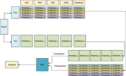
The prediction of efficiency for the pumping well system is a regression problem. The stacked integrated learning approach enables the integration of multiple diverse base learners, wherein each base learner is trained on a designated training set and utilizes its prediction outcomes as inputs for the meta-learner. Moreover, in case any of the base learners encounters an error, the meta-learner automatically rectifies it to achieve enhanced predictive performance. Therefore, in this paper, the stacking integrated learning method is chosen to predict the system efficiency of pumping wells. Since the selection of base model and metamodel is stochastic, we choose CNN, RNN, LSTM, GRU, and transformer as the base model and FNN as the metamodel. The base model is trained using the fivefold cross-validation principle. By employing the metamodel as a carrier and integrating the base model through a stacking integration strategy, we establish an efficiency prediction model for pumping systems based on fivefold cross-validation. The steps are as follows and the structure is schematized in Figure 1 and Algorithm 1.

Details are in the caption following the image — **Figure 1**
Open in figure viewer PowerPoint

Stacking integration algorithm structure diagram.

Algorithm 1: Stacking integration learning based on fivefold cross-validation.

- 1. Divide the dataset into a training set and a test set.
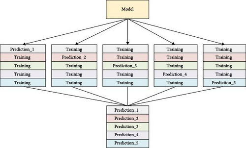
- 2. The training set in Step 1 is divided equally into five equal parts, each as a base test set and the rest as a base training set, utilizing CNN, RNN, LSTM, GRU, and transformer models, respectively. Finally, 25 different single neural network models are obtained, respectively. Each of these single networks contains five structurally different models. They are tested using a base test set and the base test results of the same network are stacked in row form. The fivefold cross-training plot for a single model is shown in Figure 2.
- 3. The predicted values of the base test set of the CNN model, the predicted values of the base test set of the RNN model, the predicted values of the base test set of the LSTM model, the predicted values of the base test set of the GRU model, and the predicted values of the base test set of the transformer model in Step 2 are arranged in columns as the training set of the metamodel.
- 4. For the construction of the test set of the metamodel, the test set of the partitioned data in Step 1 was predicted using one of the five CNN models trained in Step 2, respectively, and the values of the five prediction results were averaged to obtain the final CNN model prediction results. Repeat the above steps in the RNN network model, LSTM network model, GRU network model, and transformer network model to get the predicted results of five base model test sets, and arrange the predicted results of these five base model test sets in the form of columns to get the test sets of metamodels.
- 5. The training set of the metamodel obtained from Step 3 is substituted into the metamodel based on the fully connected neural network for training, and the test set of the metamodel obtained from Step 4 is used for test.

4. Experiments and Analyses

To enhance prediction accuracy, this paper presents a stacked ensemble learning framework that leverages fivefold cross-validation. The framework integrates five base models—CNN, RNN, LSTM, GRU, and transformer—with a metamodel that employs a FNN. To evaluate the predictive efficacy of the proposed model, the study utilizes a dataset comprising system efficiency metrics from 5,000 pumping wells in an oil field.

4.1. Data Presentation

(1)
The data for this study were obtained from a database of an oil field in the western region of the People’s Republic of China, which contains 26 impact features and one predictive feature. Among them, the pumping unit model, motor model, and balancing method are represented as string types. The stem diameter, stem length, well inclination angle, and azimuth angle are continuous numeric function types. The label encoding LabelEncoder (.) from the scikit-learn library was used to perform the encoding.
(2)
To address potential data imbalance, we randomly selected 5,000 actual wells from the database. Outliers were then removed from this subset. If fewer than 5,000 wells remained after outlier removal, additional data were selected from the source database until the total reached 5,000 wells. The dataset was then divided into a training set (80%) and a test set (20%) and normalized using Equation (24).

4.2. Pearson Correlation Coefficient Analysis

Pearson’s correlation coefficient was used to assess the impact of each important feature on the efficiency of the system and the results are shown in Table 1.

Table 1. Analysis of correlation coefficients of influencing factors.

Impact characteristics	Correlation coefficient	Impact characteristics	Correlation coefficient
Motor type	−0.009	Anticollision distance (m)	−0.015
Type of pumping unit	0.076	Oil pipe specifications (mm)	0.037
Balanced approach	−0.0092	Pump depth (m)	0.095
Balance degree (%)	−0.0041	Stroke (m)	−0.04
Saturation pressure (MPa)	−0.034	Pump diameter (mm)	0.35
Oil well fluid density (kg/m³)	0.033	Jig frequency (min⁻¹)	−0.21
Oil well fluid viscosity (MPa.s)	−0.15	Number of pumping rod stages	−0.039
Gas–oil ratio	−0.22	Sucker rod diameter (mm)	−0.052
Relative density of natural gas (kg/m³)	−0.036	Sucker rod length (m)	0.31
Oil pressure (MPa)	0.0041	Well inclination angle (angle)	0.041
Casing pressure (MPa)	0.016	Dogleg degree (angle)	−0.14
Moisture content (%)	0.2	The number of stabilizers	−0.088
Dynamic liquid level (m)	0.04	—	—
Pump clearance level	0.024	—	—

Simulation results are analyzed:

(1)
According to the analysis of Table 1, it is known that the system efficiency of the pumping unit well is negatively related to the type of motor, balancing method, balancing degree, saturation pressure, kinetic viscosity of well fluid, gas–oil ratio, the relative density of natural gas, release stroke, stroke, stroke, number of pumping rod stages, diameter of pumping rods, degree of doglegs, and number of holdups. A positive correlation exists between the type of pumping unit well, oil well fluid density, oil pressure, casing pressure, water content, dynamic liquid level, clearance level, tubular specification, down pumping depth, diameter of pumps, length of pumping rods, and inclination angle of wells and the system efficiency of the pumping unit well.
(2)
To ensure the accuracy of the prediction, this paper selects the factors affecting the efficiency of the pumping unit well system as follows: motor type, balancing method, degree of balancing, saturation pressure, kinetic viscosity of the oil well fluid, gas–oil ratio, relative density of natural gas, release stroke, stroke, number of pumping rod stages, the diameter of the pumping rods, degree of the doglegs, number of holdups, type of the pumping unit wells, the density of oil well fluids, oil pressure, casing pressure, moisture content, dynamic liquid level, clearance class of pumps, specification of the oil tubing, depth of the down-pumping, diameter of the pump, length of pumping rods, and the angle of the inclination of the wells.

4.3. Evaluation Indicators

In this study, the evaluation indices for assessing the accuracy of the prediction model for pumping system efficiency incorporate key metrics commonly employed in regression models, including mean square error (MSE), root-mean-square error (RMSE), mean absolute error (MAE), and R square (R²). The mathematical models of these evaluation indexes are as follows:

(25)

(26)

(27)

(28)

where M represents the total number of samples, y_ac,j represents the true value, and y_pr,j represents the predicted value.

4.4. Validation of Prediction Accuracy

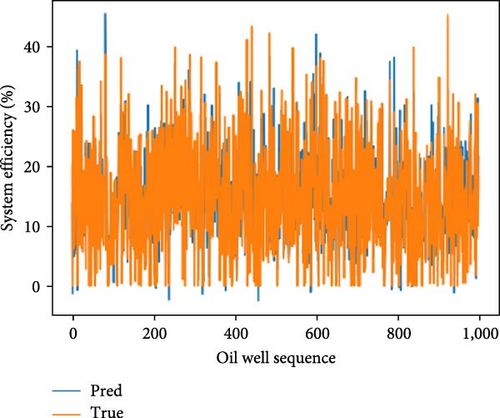
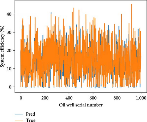
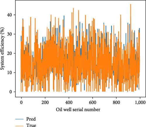
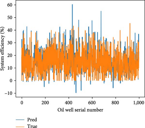
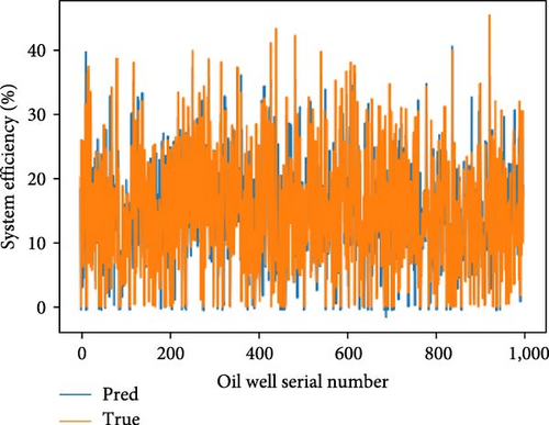
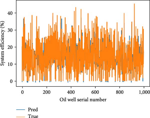
This study assesses the performance of various machine learning models in predicting oil well outputs. A training set of 4,000 oil wells and a test set of 1,000 oil wells were used. The models evaluated include CNN, RNN, LSTM, GRU, transformer, and a stacking integrated network. Predictions were made on the test set, and performance metrics are detailed in Figure 3. The results are summarized in Table 2, which presents MSE, RMSE, MAE, R², and time metrics. Improvements for each model and the integrated learning approach are analyzed in Table 3. Hyperparameter settings for each model are specified in Table 4.

Table 2. Evaluation indicators for each model.

Model	MSE	MAE	RMSE	R²	T (s)
CNN	0.00331	0.0372	0.0575	0.6193	33
RNN	0.00281	0.0323	0.0530	0.6765	281
GRU	0.00289	0.0318	0.0537	0.6674	275
Transformer	0.00317	0.0343	0.0563	0.6351	335
LSTM	0.00311	0.0324	0.0557	0.6424	236
Stacking	0.00236	0.0281	0.0485	0.7292	5,700

Table 3. Percentage improvement in evaluation metrics for single model and integrated learning.

Model	MSE (%)	MAE (%)	RMSE (%)	R² (%)
CNN	28.26	24.40	15.66	17.74
RNN	16.3	12.94	8.5	7.79
GRU	18.56	11.34	9.76	9.25
Transformer	25.78	18.05	13.85	14.81
LSTM	24.28	13.23	12.98	13.51

Table 4. Hyperparameters for each model.

Model	Learning rate	Number of hidden layers	Number of neurons in the hidden layer	Epochs	Division ratio (%)	Optimizer type
CNN	0.001	3	300	5,000	20	Adam
RNN	0.001	3	300	5,000	20	Adam
GRU	0.001	3	300	5,000	20	Adam
Transformer	0.001	3	300	5,000	20	Adam
LSTM	0.001	3	300	5,000	20	Adam
Stacking	0.001	3	300	5,000	20	Adam

Simulation results are analyzed:

(1)
Based on the experimental results presented in Figure 3, Tables 2, and 3, it is evident that the stacking model exhibits the lowest MSE, MAE, and RMSE, while demonstrating the highest R² value. This empirical evidence suggests that the predictive accuracy of the pumping unit well system efficiency prediction model based on the stacking integration strategy surpasses that of individual neural network prediction models.
(2)
The accuracy of each model is influenced not only by the hyperparameters but also by the data distribution. According to Table 2, among the single neural network prediction models, the RNN adapts better to this sample data, while the CNN shows poorer adaptation. The integrated learning model leverages the strengths of all individual neural network models to maximize its accuracy.
(3)
According to Table 2, the analysis of the learning time for each prediction model shows that the integrated learning model has the longest training time, which correlates with its higher prediction accuracy. However, in practical applications, it is common to improve one aspect of performance at the expense of less critical factors.

5. Analysis of the Impact of Hyperparameters on Accuracy and Stability

5.1. Effect of Learning Rate on Prediction Accuracy

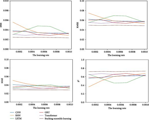
This study investigates the effect of varying learning rates on the prediction accuracy of several machine learning models. We tested learning rates of 0.0001, 0.0003, 0.0005, 0.0007, and 0.001 using CNN, RNN, LSTM, GRU, transformer, and stacking integrated learning models. Each model underwent fivefold cross-validation to assess its performance. The impact of different learning rates on model accuracy was evaluated using MSE, RMSE, MAE, and R² scores, as illustrated in Figure 4.

This can be seen from the experimental results in Figure 4:

(1)
The analysis shows that with varying learning rates, the stacking integrated learning model consistently achieved the lowest MSE, RMSE, and MAE while attaining the highest R² score. This indicates that the stacking integrated learning approach proposed in this study offers superior prediction accuracy compared to individual neural network models.
(2)
Throughout the range of learning rates, the stacking integrated learning model exhibited minimal fluctuation in all evaluation metrics. This stability suggests that the stacking integrated learning approach proposed in this study is more robust compared to individual neural network models.

5.2. Effect of the Number of Neurons in the Hidden Layer on the Prediction Accuracy

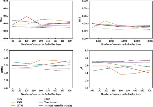
This study examines the effect of varying the number of hidden layer neurons on the predictive accuracy of integrated network models. We tested five different neuron configurations: 100, 200, 300, 400, and 500. Using a controlled variable approach, we evaluated CNN, RNN, LSTM, GRU, and transformer models, alongside stacking integrated learning models. Predictions were made using fivefold cross-validation. The performance of each model was assessed based on MSE, RMSE, MAE, and R² values, as shown in Figure 5.

This can be obtained by analyzing the experimental results according to Figure 5:

(1)
As the number of neurons in the hidden layers increases, the stacking integrated learning model demonstrates the lowest MSE, RMSE, and MAE, while achieving the highest R² value. These results indicate that the stacking integrated learning model provides superior prediction accuracy for the pumping unit well system efficiency compared to individual neural network models.
(2)
Increasing the number of neurons in the hidden layers results in minimal variations in the evaluation metrics of the stacking integrated learning model for predicting pumping unit well system efficiency. This suggests that the stacking integrated learning model exhibits greater stability compared to individual neural network models.

5.3. Effect of the Number of Hidden Layers on Prediction Accuracy

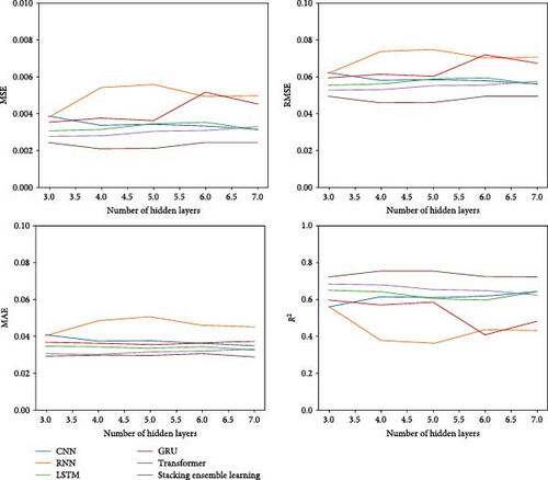
To assess the effect of varying the number of hidden layers on the predictive accuracy of integrated network models, we evaluated configurations with 3, 4, 5, 6, and 7 hidden layers. Utilizing a controlled variable approach, we applied CNN, RNN, LSTM, GRU, and transformer models, along with a stacking integrated learning model. Predictions were made using fivefold cross-validation. The performance of each model was assessed based on MSE, RMSE, MAE, and R² values, as shown in Figure 6.

This can be seen from the experimental results in Figure 6:

(1)
As the number of hidden layers increases, the stacking integrated learning model consistently achieves lower MSE, RMSE, and MAE compared to individual neural network models. Additionally, the stacking integrated learning model attains a higher R² value. These results demonstrate that the stacking integrated learning model offers superior predictive accuracy for the pumping unit well system efficiency over single neural network models.
(2)
As the number of hidden layers increases, the evaluation metrics for the stacking integrated learning model exhibit minimal variation. This suggests that the stacking integrated learning model maintains greater stability in predicting pumping unit well system efficiency compared to other models.

5.4. Effect of Epochs on Prediction Accuracy

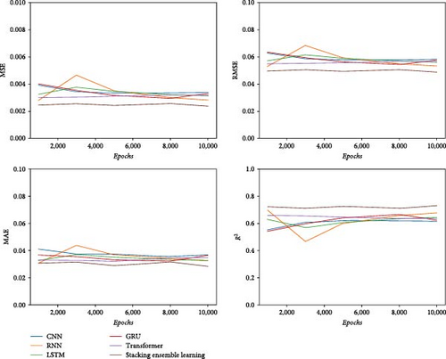
To evaluate the effect of varying the Epochs on the predictive accuracy of integrated network models, we tested configurations with 1,000, 3,000, 5,000, 8,000, and 10,000 iterations. Using a controlled variable approach, we applied CNN, RNN, LSTM, GRU, and transformer models, along with a stacking integrated network model, utilizing fivefold cross-validation. The performance of each model was assessed based on MSE, RMSE, MAE, and R² scores, as illustrated in Figure 7.

This can be obtained from the experimental results in Figure 7:

(1)
As the Epochs increases, the stacking integrated learning model consistently achieves the lowest MSE, RMSE, and MAE, while attaining the highest R² value. These findings indicate that the stacking integrated learning model offers superior predictive accuracy for pumping unit well system efficiency compared to single neural network models.
(2)
The evaluation metrics for the stacking integrated learning model exhibit minimal variation with increasing Epochs, indicating that this model maintains a higher level of stability compared to others.

5.5. Effect of the Division Ratio of the Validation Set on the Prediction Accuracy

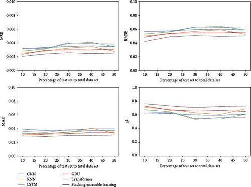
To evaluate the effect of different validation set division ratios on the predictive accuracy of integrated network models, we analyzed division ratios of 0.1, 0.2, 0.3, 0.4, and 0.5. Using a controlled variable approach, we applied CNN, RNN, LSTM, GRU, and transformer models, along with a stacking integrated network model, utilizing fivefold cross-validation. The performance of each model was assessed using MSE, RMSE, MAE, and the coefficient of determination R², as illustrated in Figure 8.

This can be obtained by analyzing the experimental results according to Figure 8:

(1)
As the proportion of the validation set increases, the stacking integrated learning model consistently achieves lower MSE, RMSE, and MAE compared to single neural network models. This indicates that the stacking integrated learning model provides superior predictive accuracy for pumping unit well system efficiency.
(2)
With an increased proportion of validation set data, the stacking integrated learning model shows reduced variation in evaluation metrics compared to single neural network models. This suggests that the stacking integrated learning model offers greater stability for predicting pumping unit well system efficiency

6. Conclusion

(1)
This study introduces a novel prediction model for the efficiency of pumping well systems based on stacking integrated learning. The model consists of a base model and a metamodel. The base model integrates various neural network architectures, including CNN, RNN, LSTM, GRU, and transformer models. The metamodel is designed as a FNN. Initially, we performed a quantitative analysis of the factors influencing pumping well system efficiency using the Pearson correlation coefficient. Data preprocessing was then conducted through min–max normalization. Finally, a fivefold cross-validation technique was employed to train the base model, and the stacking integration strategy was applied, with a fully connected neural network serving as the metamodel. This approach resulted in an efficient prediction model for pumping well system performance.
(2)
To validate the model’s accuracy, experiments were conducted on a sample of 5,000 real oil wells. The experimental findings demonstrate that the predictive accuracy of the stacking integrated learning-based model for pumping well system efficiency surpasses that of individual neural network models.
(3)
To analyze the stability of the model, we examined the effects of learning rate, number of hidden layers, number of neurons in the hidden layer, total number of iteration steps, and the proportion of validation set division using the control variable method. The results indicate that the stacking integrated learning-based prediction model for pumping well system efficiency proposed in this paper exhibits greater stability compared to individual neural network models.
(4)
Predicting the efficiency of pumping well systems is crucial for petroleum practitioners to evaluate the performance of these systems. Given that different integration strategies yield varying levels of predictive accuracy, future research will primarily focus on investigating the effects of different integration strategies on the prediction accuracy of pumping unit well system efficiency.

Conflicts of Interest

The authors declared that they have no conflicts of interest to this work. We declare that we do not have any commercial or associative interest that represents a conflicts of interest in connection with the work submitted.

Acknowledgments

This research was funded by the National Natural Science Foundation of China (grant no. 51974276).

Open Research

Data Availability

The dataset generated and analyzed during the current research period will be provided within the scope of informed consent of the first author upon reasonable academic request.

References

1 Gibbs S. G., Predicting the behavior of sucker rod pumping systems, Journal of Petroleum Technology. 6, no. 10, 1–10, https://doi.org/10.2118/588-PA.
10.2118/588-PA
Google Scholar
2 Doty D. R. and Schmidt Z., An improved model for sucker rod pumping, Society of Petroleum Engineers Journal. (1983) 23, no. 1, 33–41, https://doi.org/10.2118/10249-PA, 2-s2.0-0020501688.
10.2118/10249-PA
Google Scholar
3 Lekia S. D. and Evans R. D., A coupled rod and fluid dynamic model for predicting the behavior of sucker-rod pumping systems—part 2: parametric study and demonstration of model capabilities, SPE Production & Facilities. (1995) 10, no. 1, 34–40, https://doi.org/10.2118/30169-PA.
10.2118/30169-PA
CAS Google Scholar
4 Xing M., Zhou L., Zhang C., Xue K., and Zhang Z., Simulation analysis of nonlinear friction of rod string in sucker rod pumping system, Journal of Computational and Nonlinear Dynamics. (2019) 14, no. 9, https://doi.org/10.1115/1.4044027, 2-s2.0-85069161564.
10.1115/1.4044027
Web of Science® Google Scholar
5 Li Q., Chen B., Huang Z., Tang H., Li G., and He L., Study on equivalent viscous damping coefficient of sucker rod based on the principle of equal friction loss, Mathematical Problems in Engineering. (2019) 2019, no. 1, 12, https://doi.org/10.1155/2019/9272751, 2-s2.0-85065259308, 9272751.
10.1155/2019/9272751
Web of Science® Google Scholar
6 Xing M., Response analysis of longitudinal vibration of sucker rod string considering rod buckling, Advances in Engineering Software. (2016) 99, 49–58, https://doi.org/10.1016/j.advengsoft.2016.05.004, 2-s2.0-84969204334.
10.1016/j.advengsoft.2016.05.004
Web of Science® Google Scholar
7 Wang X., Lv L., Li S., Pu H., Liu Y., Bian B., and Li D., Longitudinal vibration analysis of sucker rod based on a simplified thermo-solid model, Journal of Petroleum Science and Engineering. (2021) 196, https://doi.org/10.1016/j.petrol.2020.107951, 107951.
10.1016/j.petrol.2020.107951
CAS Web of Science® Google Scholar
8 Wang H. and Dong S., Research on the coupled axial-transverse nonlinear vibration of sucker rod string in deviated wells, Journal of Vibration Engineering & Technologies. (2021) 9, no. 1, 115–129, https://doi.org/10.1007/s42417-020-00214-5.
10.1007/s42417-020-00214-5
Web of Science® Google Scholar
9 Yin J.-J., Sun D., and Yang Y.-S., Predicting multi-tapered sucker-rod pumping systems with the analytical solution, Journal of Petroleum Science and Engineering. (2021) 197, https://doi.org/10.1016/j.petrol.2020.108115, 108115.
10.1016/j.petrol.2020.108115
CAS Web of Science® Google Scholar
10 Dong S., Li W., Houtian B., Wang H., Chen J., and Liu M., Optimizing the running parameters of a variable frequency beam pumping system and simulating its dynamic behaviors, Journal of Mechanical Engineering. (2016) 52, no. 21, 63–70, https://doi.org/10.3901/JME.2016.21.063, 2-s2.0-85012279053.
10.3901/JME.2016.21.063
Google Scholar
11 Tarmigh M., Behbahani-Nejad M., and Hajidavalloo E., Two-way fluid-structure interaction for longitudinal vibration of a loaded elastic rod within a multiphase fluid flow, Journal of the Brazilian Society of Mechanical Sciences and Engineering. (2023) 45, no. 11.
10.1007/s40430-023-04484-4
Web of Science® Google Scholar
12 Ma B., Coupling simulation of longitudinal vibration of rod string and multi-phase pipe flow in wellbore and research on downhole energy efficiency, Energies. (2023) 16, no. 13, https://doi.org/10.3390/en16134988, 4988.
10.3390/en16134988
CAS Web of Science® Google Scholar
13 Moreno G. A. and Garriz A. E., Sucker rod string dynamics in deviated wells, Journal of Petroleum Science and Engineering184. (2020) 184, https://doi.org/10.1016/j.petrol.2019.106534, 106534.
10.1016/j.petrol.2019.106534
CAS Web of Science® Google Scholar
14 Guo X., Zhu C., Hao J., and Zhang S., Multi-step wind speed prediction based on an improved multi-objective seagull optimization algorithm and a multi-kernel extreme learning machine, Applied Intelligence. (2023) 53, no. 13, 16445–16472, https://doi.org/10.1007/s10489-022-04312-7.
10.1007/s10489-022-04312-7
Web of Science® Google Scholar
15 Xing Z., Zhao R., Wu Y., and He T., Intelligent fault diagnosis of rolling bearing based on novel CNN model considering data imbalance, Applied Intelligence. (2022) 52, no. 14, 16281–16293, https://doi.org/10.1007/s10489-022-03196-x.
10.1007/s10489-022-03196-x
Web of Science® Google Scholar
16 Yin P., A multiscale graph convolutional neural network framework for fault diagnosis of rolling bearing, IEEE Transactions on Instrumentation and Measurement. (2023) 72, 1–13.
PubMed Web of Science® Google Scholar
17 Liu K., Zheng M., Liu Y., Yang J., and Yao Y., Deep autoencoder thermography for defect detection of carbon fiber composites, IEEE Transactions on Industrial Informatics. (2023) 19, no. 5, 6429–6438, https://doi.org/10.1109/TII.2022.3172902.
10.1109/TII.2022.3172902
Web of Science® Google Scholar
18 Sun Z., Yao Q., Jin H., Xu Y., Hang W., Chen H., Li K., Shi L., Gu J., Zhang Q., and Zhen X., A novel in-situ sensor calibration method for building thermal systems based on virtual samples and autoencoder, Energy. (2024) 297, 131314.
10.1016/j.energy.2024.131314
Web of Science® Google Scholar
19 Zhao Z., Chen W., Wu X., Chen P. C. Y., and Liu J., LSTM network: a deep learning approach for short-term traffic forecast, IET Intelligent Transport Systems. (2017) 11, no. 2, 68–75, https://doi.org/10.1049/iet-its.2016.0208, 2-s2.0-85015163282.
10.1049/iet-its.2016.0208
Web of Science® Google Scholar
20 Wang F., Zhang Z., Liu C., Yu Y., Pang S., Duić N., Shafie-Khah M., and Catalão J. P. S., Generative adversarial networks and convolutional neural networks based weather classification model for day ahead short-term photovoltaic power forecasting, Energy Conversion and Management. (2019) 181, 443–462, https://doi.org/10.1016/j.enconman.2018.11.074, 2-s2.0-85058686522.
10.1016/j.enconman.2018.11.074
Web of Science® Google Scholar
21 Acharya U. R., Fujita H., Oh S. L., Hagiwara Y., Tan J. H., Adam M., and Tan R. S., Deep convolutional neural network for the automated diagnosis of congestive heart failure using ECG signals, Applied Intelligence. (2019) 49, no. 1, 16–27, https://doi.org/10.1007/s10489-018-1179-1, 2-s2.0-85046028708.
10.1007/s10489-018-1179-1
Web of Science® Google Scholar
22 An Z., Wang X., Li B., Xiang Z., and Zhang B., Robust visual tracking for UAVs with dynamic feature weight selection, Applied Intelligence. (2023) 53, no. 4, 3836–3849, https://doi.org/10.1007/s10489-022-03719-6.
10.1007/s10489-022-03719-6
Web of Science® Google Scholar
23 Zhang Z., Lu B., Xu X., Shen X., Feng J., and Brunauer G., CN-MgMP: a multi-granularity module partition approach for complex mechanical products based on complex network, Applied Intelligence. (2023) 53, no. 14, 17679–17692, https://doi.org/10.1007/s10489-022-04430-2.
10.1007/s10489-022-04430-2
Web of Science® Google Scholar
24 Wang X., Li X., and Li S., A novel stock indices hybrid forecasting system based on features extraction and multi-objective optimizer, Applied Intelligence. (2022) 52, no. 10, 11784–11807, https://doi.org/10.1007/s10489-021-03031-9.
10.1007/s10489-021-03031-9
Web of Science® Google Scholar
25 Huang Z., Li K., Ke C., Duan H., and Wang M., An intelligent diagnosis method for oil-well pump leakage fault in oilfield production internet of things system based on convolutional attention residual learning, Engineering Applications of Artificial Intelligence. 126, 106829.
10.1016/j.engappai.2023.106829
Web of Science® Google Scholar
26 Lv X. X., Wang H. X., and Zhang X., An evolutional SVM method based on incremental algorithm and simulated indicator diagrams for fault diagnosis in sucker rod pumping systems, Journal of Petroleum Science and Engineering, 2021, 203.
Google Scholar
27 Zhang K., Wang Q., and Wang L. B., Fault diagnosis method for sucker rod well with few shots based on meta-transfer learning, Journal of Petroleum Science and Engineering. (2022) 212, https://doi.org/10.1016/j.petrol.2022.110295, 110295.
10.1016/j.petrol.2022.110295
CAS Web of Science® Google Scholar
28 Zhang A. and Gao X., Supervised dictionary-based transfer subspace learning and applications for fault diagnosis of sucker rod pumping systems, Neurocomputing. (2019) 338, no. 338, 293–306, https://doi.org/10.1016/j.neucom.2019.02.013, 2-s2.0-85061652291.
10.1016/j.neucom.2019.02.013
Web of Science® Google Scholar
29 Han Y., Li K., Ge F., Wang Y’an, and Xu W., Online fault diagnosis for sucker rod pumping well by optimized density peak clustering, ISA Transactions. (2022) 120, no. 120, 222–234, https://doi.org/10.1016/j.isatra.2021.03.022.
10.1016/j.isatra.2021.03.022
PubMed Web of Science® Google Scholar
30 Jiang C., Fang S., and Liu W., Production prediction of extra high water cut oil well based on convolution neural network and transfer learning, Zhongguo Shiyou Daxue Xuebao (Ziran Kexue Ban)/Journal of China University of Petroleum. (2023) 47, no. 6, 162–170, https://doi.org/10.3969/j.issn.1673-5005.2023.06.019.
10.3969/j.issn.1673-5005.2023.06.019
Google Scholar
31 Yi P., Chunming X., Jianjun Z., Yashun Z., Qinming G., Guojian X., Xishun Z., Ruidong Z., Junfeng S., Meng L., Cai W., and Guanhong C., Innovative deep autoencoder and machine learning algorithms applied in production metering for sucker-rod pumping, SPE/AAPG/SEG Unconventional Resources Technology Conference. (2019) https://doi.org/10.15530/urtec-2019-1090, 2-s2.0-85072925571.
10.15530/urtec-2019-1090
Google Scholar
32 Pan S. W., Yang B., and Wang S. K., Oil well production prediction based on CNN-LSTM model with self-attention mechanism, Energy. (2023) 284, 128701.
10.1016/j.energy.2023.128701
Web of Science® Google Scholar
33 Lei Z., Hongen D., Tianzhi W., Hongliang W., Yi P., Jifeng Z., Zongshang L., Lan M., and Liwei J., A production prediction method of single well in water flooding oilfield based on integrated temporal convolutional network model, Petroleum Exploration and Development. 49, no. 5, 1150–1160.
Web of Science® Google Scholar
34 Cheng Y. and Yang Y., Prediction of oil well production based on the time series model of optimized recursive neural network, Petroleum Science and Technology. (2021) 39, no. 9-10, 303–312, https://doi.org/10.1080/10916466.2021.1877303.
10.1080/10916466.2021.1877303
CAS Web of Science® Google Scholar
35 Zhou G. Z., Guo Z. Q., and Sun S. M., A CNN-BiGRU-AM neural network for AI applications in shale oil production prediction, Applied Energy, 2023, 334.
Google Scholar
36 Lu Q., Wang S., Jiang M., Li Y., and Dong K., Main control factors affecting mechanical oil recovery efficiency in complex blocks identified using the improved k-means algorithm, PLOS ONE. (2021) 16, no. 5, https://doi.org/10.1371/journal.pone.0248840, e0248840.
10.1371/journal.pone.0248840
CAS PubMed Web of Science® Google Scholar
37 Tan C., Deng H., Feng Z., Li B., Peng Z., and Feng G., Data-driven system efficiency prediction and production parameter optimization for PW-LHM, Journal of Petroleum Science and Engineering. (2022) 209, https://doi.org/10.1016/j.petrol.2021.109810, 109810.
10.1016/j.petrol.2021.109810
CAS Web of Science® Google Scholar
38 Lin S., Zheng H., Han B., Li Y., Han C., and Li W., Comparative performance of eight ensemble learning approaches for the development of models of slope stability prediction, Acta Geotechnica. (2022) 17, no. 4, 1477–1502, https://doi.org/10.1007/s11440-021-01440-1.
10.1007/s11440-021-01440-1
Web of Science® Google Scholar
39 Xiao Y., Wu J., Lin Z., and Zhao X., A deep learning-based multi-model ensemble method for cancer prediction, Computer Methods and Programs in Biomedicine. (2018) 153, 1–9, https://doi.org/10.1016/j.cmpb.2017.09.005, 2-s2.0-85030330677.
10.1016/j.cmpb.2017.09.005
PubMed Web of Science® Google Scholar
40 Chen J., Zeng G.-Q., Zhou W., Du W., and Lu K.-D., Wind speed forecasting using nonlinear-learning ensemble of deep learning time series prediction and extremal optimization, Energy Conversion and Management. (2018) 165, 681–695, https://doi.org/10.1016/j.enconman.2018.03.098, 2-s2.0-85044921561.
10.1016/j.enconman.2018.03.098
Web of Science® Google Scholar
41 Onan A., Korukoğlu S., and Bulut H., A multiobjective weighted voting ensemble classifier based on differential evolution algorithm for text sentiment classification, Expert Systems with Applications. (2016) 62, 1–16, https://doi.org/10.1016/j.eswa.2016.06.005, 2-s2.0-84977070618.
10.1016/j.eswa.2016.06.005
Web of Science® Google Scholar
42 Kardani N., Zhou A., Nazem M., and Shen S.-L., Improved prediction of slope stability using a hybrid stacking ensemble method based on finite element analysis and field data, Journal of Rock Mechanics and Geotechnical Engineering. (2021) 13, no. 1, 188–201, https://doi.org/10.1016/j.jrmge.2020.05.011.
10.1016/j.jrmge.2020.05.011
Web of Science® Google Scholar
43 Xie Y., Sun W., Ren M., Chen S., Huang Z., and Pan X., Stacking ensemble learning models for daily runoff prediction using 1D and 2D CNNs, Expert Systems with Applications. (2023) 217, https://doi.org/10.1016/j.eswa.2022.119469, 119469.
10.1016/j.eswa.2022.119469
Web of Science® Google Scholar
44 Atha D. J., Jahanshahi MR(2018)Evaluation of deep learning approaches based on convolutional neural networks for corrosion, Structural Health Monitoring. (2018) 17, no. 5, 1110–1128, https://doi.org/10.1177/1475921717737051, 2-s2.0-85042103996.
10.1177/1475921717737051
Web of Science® Google Scholar
45 Liu Y., Xiao H., Xu J., and Zhao J., A rail surface defect detection method based on pyramid feature and lightweight convolutional neural network, IEEE Transactions on Instrumentation and Measurement. (2022) 71, 1–10, https://doi.org/10.1109/TIM.2022.3219307.
10.1109/TIM.2022.3219307
Web of Science® Google Scholar
46 Sherstinsky A., Fundamentals of recurrent neural network (RNN) and long short-term memory (LSTM) network, Physica D: Nonlinear Phenomena. (2020) 404, https://doi.org/10.1016/j.physd.2019.132306, 132306.
10.1016/j.physd.2019.132306
Web of Science® Google Scholar
47 Zhang B., Zhang S., and Li W., Bearing performance degradation assessment using long short-term memory recurrent network, Computers in Industry. (2019) 106, 14–29, https://doi.org/10.1016/j.compind.2018.12.016, 2-s2.0-85059203515.
10.1016/j.compind.2018.12.016
Web of Science® Google Scholar
48 Cui Z., Ke R., Pu Z., and Wang Y., Stacked bidirectional and unidirectional LSTM recurrent neural network for forecasting network-wide traffic state with missing values, Transportation Research Part C: Emerging Technologies. (2020) 118, https://doi.org/10.1016/j.trc.2020.102674, 102674.
10.1016/j.trc.2020.102674
Web of Science® Google Scholar
49 Karevan Z. and Suykens J. A. K., Transductive LSTM for time-series prediction: an application to weather forecasting, Neural Networks. (2020) 125, 1–9, https://doi.org/10.1016/j.neunet.2019.12.030.
10.1016/j.neunet.2019.12.030
PubMed Web of Science® Google Scholar
50 Zhao L., Li Z., Qu L., Zhang J., and Teng B., A hybrid VMD-LSTM/GRU model to predict non-stationary and irregular waves on the east coast of China, Ocean Engineering. (2023) 276, https://doi.org/10.1016/j.oceaneng.2023.114136, 114136.
10.1016/j.oceaneng.2023.114136
Web of Science® Google Scholar
51 Wang Y.-X., Chen Z., and Zhang W., Lithium-ion battery state-of-charge estimation for small target sample sets using the improved GRU-based transfer learning, Energy. (2022) 244, https://doi.org/10.1016/j.energy.2022.123178, 123178.
10.1016/j.energy.2022.123178
Web of Science® Google Scholar
52 Xu P., Zhu X., and Clifton D. A., Multimodal learning with transformers: a survey, IEEE Transactions on Pattern Analysis and Machine Intelligence. (2023) 45, no. 10, 12113–12132, https://doi.org/10.1109/TPAMI.2023.3275156.
10.1109/TPAMI.2023.3275156
PubMed Web of Science® Google Scholar
53 Shamshad F., Khan S., Zamir S. W., Khan M. H., Hayat M., Khan F. S., and Fu H., Transformers in medical imaging: a survey, Medical Image Analysis. (2023) 88, https://doi.org/10.1016/j.media.2023.102802, 102802.
10.1016/j.media.2023.102802
PubMed Web of Science® Google Scholar
54 Zhou H., Deng Z., Xia Y., and Fu M., A new sampling method in particle filter based on Pearson correlation coefficient, Neurocomputing. 216, 208–215.
10.1016/j.neucom.2016.07.036
Web of Science® Google Scholar

Citing Literature

All articles

A Hybrid Prediction Model for Pumping Well System Efficiency Based on Stacking Integration Strategy

Abstract

1. Introduction