In this study, we proposed and analyzed a nonlinear deterministic mathematical model of malaria transmission dynamics. In addition to the previous approaches, we incorporated the class of aware people and other control measures. We established the wellposedness of the model, and the asymptotic behavior of the solutions is rigorously studied depending on the basic reproduction number R₀. The model system admits two equilibrium points: disease-free and disease-persistent equilibrium points. The analytical result of the model system revealed that the disease-free equilibrium point is both locally as well as globally asymptotically stable whenever R₀ < 1 while the disease-persistence equilibrium point is globally asymptotically stable whenever R₀ > 1. Moreover, the forward bifurcation phenomenon of the model system for R₀ = 1 was analyzed by using center manifold theory. A sensitivity analysis of the basic reproduction number was performed to identify parameters that will cause to trigger the transmission of malaria disease and should be targeted by control strategies. Then, the model was extended to the optimal control problem, with the use of three time-dependent controls, namely, preventive measures(treated bednets and indoor residual spraying), continuous awareness campaigns to susceptible individuals, and treatment for infected individuals. By using Pontryan’s maximum principle, necessary conditions for the transmission of malaria disease were derived. Numerical simulations are illustrated by using MATLAB ode45 to validate the theoretical results of the model. The numerical findings of the optimal model suggested that integrated control strategies are better than a sole intervention to eliminate malaria disease.

1. Introduction

Nowadays, developing countries are challenging with a lot of problems, such as climatic change, racism, terrorism, unemployment, poverty, and public health crises. Among them, malaria disease is continued as a killer death and a major public health issue [1]. It is a contagious illness and spreads between people through the bites of infected female Anopheles mosquitoes [2, 3]. The most common species that can cause to human illness are Plasmodium vivax, plasmodium falciparum, Plasmodium ovale, Plasmodium malariae, and Plasmodium knowles, and their distribution may vary from place to place [1]. The most common symptoms of malaria include high fever, joint pains, abdominal pains, headaches, vomiting, nausea, diarrhea, and extreme fatigue [3, 4, 5, 6, 7]. Approximately 241 million cases and 627,000 deaths were reported globally in 2020, with 95% of cases occurring in the African Region [8]. Utilizing bed nets that have been treated, antimalarial drugs, and indoor residual spraying are among the most effective malaria prevention measures [9].

A thorough understanding of the disease’s transmission process and its control is necessary to create effective intervention measures and mitigations. Mathematical models help in describing the evolution of infectious diseases [10, 11, 12, 13, 14, 15, 16, 17, 18]. The first published paper on the dynamics of malaria that demonstrates the life cycle of the malaria parasite dates back to Sir Ross [19], which is SIR type. Recently, various scholars have studied the dynamics of malaria transmission using mathematical modeling approaches to combat it. For example, in 2022, Collins and Duffy [20] proposed and analyzed the dynamics of the malaria transmission model in Nigeria that takes into account drug resistance, treatment, and the use of mosquito nets as preventative measures. Their findings confirmed that unless better control strategies are put into place, the disease is likely to remain endemic in Nigeria. In 2021, Keno et al. [21] developed and analyzed a mathematical model of malaria transmission with optimal controls. Their study showed that the most cost-effective ways to reduce malaria transmission are through the combination of control measures, such as treatment and indoor residual spraying. In 2020, Ghosh et al. [17] formulated and analyzed SEIRS for human populations and SEI for vector populations with optimal control and relapse. Their result revealed that treated bed nets and indoor residue springs are the best strategies to eliminate malaria transmission. In 2018, Leiton et al. [22] presented an SEIRS-SI mathematical model for malaria transmission with optimal control in Colombia. Their finding concluded that to prevent malaria transmission the integrated control strategies must hold effectively. In 2022, Keno et al. [23] presented a nonlinear mathematical model of malaria transmission with three control strategies, namely treated bed nets, treatment, and indoor residual spraying. Both forward and backward bifurcation were present in their model, and (treatment and treated bed nets) are the best ways to reduce the burden of malaria transmission among control measures. In 2022, Gautam et al. [24] developed a mathematical model for malaria transmission dynamics that included cross-border travel between a low-endemic country (Nepal) and a high-endemic country (India) with optimal control. They reaffirmed that their study offers crucial insights into a potential barrier that cross-border mobility may pose to malaria elimination programs. Even though most countries have policies or strategies that are being made to eradicate malaria disease, it is continued as a challenge, especially for developing countries. For the best of our knowledge, mathematical models that deal with the impact of awareness creation for susceptible individuals are very rare. Thus, we are motivated to fill this gap and consider other alternative control measures.

The remaining parts of this study are outlined as follows: The model description and underlying assumptions are covered in Section 2. The basic properties of the model are discussed in Section 3. An analysis of the model is given in Section 4. The optimal control problem is presented in Section 5. Numerical simulations and discussions of the model are covered in Section 6. The conclusion is provided in Section 7.

2. Mathematical Model Formulation and Description

The model formulation is adopted from [25] by making some modifications by adding the class of aware individuals compartment for controlling malaria disease, and it makes the entire of human population to be divided into four epidemiological compartments, namely, susceptible individuals S_h(t); aware susceptible individuals A_h(t); infectious individuals I_h(t); and recovered individuals R_h(t). Furthermore, the total number of mosquitoes is classified into two groups: susceptible mosquitoes S_m(t) and infected mosquitoes I_m(t). The following assumptions are taken into account in the formulation of our model.

(i)
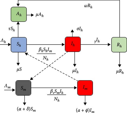
We assumed that all newly recruited humans and mosquitoes are not carriers of malaria infection.
(ii)
We considered only female anapheles mosquitoes in our recent study.
(iii)
In addition to natural death, we assumed that other human activities contribute for the mortality of mosquitoes.
(iv)
We assumed that mosquitoes feed only human blood, and vertical transmission of the infection between them is not under consideration.
(v)
We assumed that infected mosquitoes remain infectious until they die.

Keeping the above discussions in mind, the new model is portrayed in Figure 1, and state variables and parameters are presented in Tables 1 and 2, respectively.

Table 1. State variables of the model and its description.

Notation	Description
S_h(t)	The class of susceptible human population at given time t
A_h(t)	The class of aware human population at a given time t
I_h(t)	The class of infectious human population at a given time t
R_h(t)	The class of recovered human population at a given time t
S_m(t)	The class of susceptible female Anopheles mosquitoes at a given time t
I_m(t)	The class of infectious female Anopheles mosquitoes at a given time t

Table 2. Model parameters and its description.

Notation	Description
Λ_h	The recruitment rate of susceptible individuals
Λ_m	The recruitment rate of susceptible female Anopheles mosquitoes population
τ	The progression rate of susceptible individuals into the class of aware individuals
β_h	The rate in which susceptible humans get infected by infected mosquitoes
β_m	The rate in which susceptible mosquitoes get infected by infectious individuals
μ	The natural death rate of individuals
α	The natural death rate of mosquitoes
σ	The disease induced-death rate of infectious individuals
ω	The progression rate of recovered individuals to the class of aware individuals
γ	The recovery rate of infectious individuals
δ	The mortality rate of susceptible mosquitoes population due to human activities
ϕ	The mortality rate of infected mosquitoes population due to human activities

Details are in the caption following the image — **Figure 1**
Open in figure viewer PowerPoint

The flowchart of malaria transmission model.

The governing nonlinear differential equations of the model, as per the flowchart, are as follows:

()

with initial conditions:

()

and

()

3. Basic Properties of the Model

Lemma 1 (Existence and Uniqueness of Model Solutions). The unique solution in , is admissible for the model system (1) with initial condition (2).

Proof. we can rewrite the system (1) in the form of , where

()

It is straightforward to see that all the right-hand-side components of the function f (x) are continuously differentiable almost everywhere in , which implies that f (x) is of a class C¹ on for all t ≥ 0. Hence, by Picard–Lindelôf theorem [26], the model system (1) has a unique solution locally in for all t ≥ 0. This completes the proof.

Since we are dealing with populations, it is necessary to ensure the nonnegativity and boundedness of model solutions.

Lemma 2 (Nonnegativity of Model Solutions). The solution set {S_h(t), A_h(t), I_h(t), R_h(t), S_m(t), I_m(t)} of model system (1) remains nonnegative for all future time, t ≥ 0 under the initial condition (2) in the closed region .

Proof. Consider the 1st equation in the system (1),

()

Then, after solving for S_h(t), we obtained the following:

()

for all time t ≥ 0, where the function η(t) is the integrating factor given as follows:

()

From Equation (6), it is clear that the function S_h(t) is positive for all t ≥ 0, since η(t) > 0.

Likewise, consider the 5th equation in the system (1)

()

Then, after solving Equation (9), the result can be implicitly expressed as follows:

()

for all time t ≥ 0, where the function κ(t) is the integrating factor given by the following:

()

Hence, from Equation (9), the function S_m(t) is also positive for all time t ≥ 0. It can be shown in similar way that: A_h ≥ 0, I_h ≥ 0, R_h ≥ 0 and I_m ≥ 0. Therefore, all the solutions that start in the positive region remain positive.

Lemma 3 (Boundedness of Model Solutions). The malaria model (1) with initial condition (2) in is positively invariant in the feasible region , where

()

Proof. Adding all the model equations of (1), we obtain the following:

()

The positivity of model equations (1) helps us to arrive from

()

Solving the differential inequality, we obtained the relation as follows:

()

, then we can claim that

for all t ≥ 0. This confirms that the feasible solution set of the human population is given by the following:

Similarly, the time derivative of the total mosquito population, N_m(t) along model solutions (1), is obtained and given in compact form by the following:

()

Therefore, the proof of the theorem is already completed.

4. Analytical Analysis of the Model

4.1. Malaria Disease Free-Equilibrium (DFE) Point

To obtain the DFE, we set the right-hand sides of model system (1) to zero at I_h = I_m = 0. Thus, the DFE point of the model is denoted by D_f and given by the following:

4.2. Basic Reproduction Number

This section devotes to find the basic reproductive number R₀, which is an important ratio used to predict the asymptotic behavior of the disease distribution. It is defined as the average number of new cases resulted when a single infection is introduced into completely susceptible populations. We compute R₀ based on [27, 28] and denoting the vector for the newly infected by N and the rate of transfer by T where

()

The Jacobian matrix of N and T at DFE point D_f are given by F and V, where

()

Then, the inverse of V is computed and given by the following:

()

Finally, the next-generation matrix is given by the following:

()

The two eigenvalues of FV⁻¹ are as follows:

()

Indeed, the spectral radius of FV⁻¹ is as follows:

()

4.3. Malaria Disease Persistent Equilibrium Point of the Model

The disease persistent equilibrium point of the model system (1) is denoted by D_p with

. To find the components of D_p, we take all the right hand-sides of system (1) equal to zero at I_h ≠ 0, I_m ≠ 0 as follows:

()

From the first equation of system (1), we have that

()

and also from the fifth equation of system (1), we have the following:

()

Then, substituting Equation (24) into the sixth equation of system (1) yields

()

At the end, substituting Equations (23) and (25) into the third equation of system (1) and solving for

results

()

provided that

()

The remaining components of D_p are calculated based on the expression

as follows:

()

where

()

4.4. Stability Analysis of Model Equilibrium Points

In the subsequent theorems, we will examine the obtained equilibria, which are D_f and D_p of model system (1), both in local and global sense.

Theorem 1. The malaria-free equilibrium point of model system (1), is locally asymptotically stable whenever R₀ < 1 otherwise unstable.

Proof. The Jacobian matrix of the system (1) from DFE, D_f, is given by the following:

()

The charactersitics equation |J(D_f) − λI_2×2| = 0 admits four eigenvalues:

()

and the remaining eigenvalues of J(D_f) are determined from the submatrix

()

The characteristic polynomial of J₅(D_f) is expressed by the following:

()

where

()

Thus,

provided that

, which leads to R₀ < 1. According to Routh–Hurwitz criteria, it can be seen that the characteristic polynomial φ(λ) has all negative real roots whenever R₀ < 1. Hence, the DFE point D_f is locally asymptotically stable. But for R₀ > 1, there is sign change on A₂, and D_f is unstable. The epidemiological implication of this theorem is that the transmission of malaria can be controlled from the community when R₀ < 1; otherwise, reinvasion will occur within the society.

Theorem 2. The DFE point of model system (1) is globally asymptotically stable whenever R₀ < 1 otherwise unstable.

Proof. To evaluate the global stability of D_f of model system (1), we formulate a suitable Lyapunov function

()

It is easy to observe that L is of class C¹ on the interior of Δ, and the time derivative of L along the solutions of Equation (1) is given by the following:

()

Here,

since R₀ < 1 and

. Hence, L is a Lyapunov function on Δ. Additionally, the singleton set D_f is the largest compact invariant set in

. As a result, by LaSalle’s invariant principle [29], D_f is globally asymptotically stable in the interior of Δ for R₀ < 1.

Theorem 3. The disease persistent equilibrium point of the model system (1) is globally asymptotically stable on Δ for R₀ > 1.

Proof. To prove this theorem, we employ the Dulac’s criterion [30] by taking as the candidate of Dulac’s function for model system (1) and

Γ = (S_h, A_h.I_h, R_h, S_m, I_m).

Since ϱ(I_h, I_m) > 0, ∀I_h, I_m > 0, we have that

()

Then, we have that

()

This implies Dulac’s function ϱ, and model system (1) does not contain any periodic orbits in

. As a result, whenever R₀ > 1, the disease persistent equilibrium point D_p is globally asymptotically stable. In epidemiological point of view, the above result suggests that there will be fluctuation in the transmission of malaria in society, which makes it challenging to allocate resources for the control of malaria transmission.

4.5. Bifurcation Analysis of the Model

In this section, we look at the concept of the bifurcation, which includes the infection-free equilibrium, D_f at R₀ = 1, by employing Center Manifold theory [31] for system (1). To apply this, variable changes are made on the system (1) as follows S_h = x₁, A_h = x₂, I_h = x₃, R_h = x₄, S_m = x₅ and I_m = x₆, so that N_h = x₁ + x₂ + x₃ + x₄. Further, by using vector notation

, the model system (1) can be written as

where

()

The approach consists of evaluating the system’s linearized matrix (39) at the DFE point, D_f, which is given by the following:

()

If we choose

as the bifurcation parameter for R₀ = 1, then the solution to the problem of finding β_h from R₀ = 1 gives

. After some algebraic manuplations on Equation (40), the Jacobian of the system

has eigenvalues

()

which indicates that it has a single simple zero eigenvalue and that all other eigenvalues are real and negative. Therefore, the DFE is a nonhyperbolic equilibrium for

. With the above simple zero eigenvalue, Jw = 0 determines the right eigenvector,

, where

()

The left eigenvectors ν = (ν₁, ν₂, ν₃, ν₄, ν₅, ν₆) that correspond to the simple zero eigenvalues above are obtained from νJ = 0 and are given by the following:

()

which suggests that ν₆ is free. Let x_k represent state variables for k = 1, 2, 3, 4, 5, 6, and let f_k represent the kth component of the right-hand sides of model (1). The signs of the two coefficients a and b, which are completely responsible for the local dynamics of system (1) around D_f, where

()

According to the left eigenvector, we then have that

()

and

()

Since the coefficient a < 0 and b > 0, the model experiences forward bifurcation, which suggests that R₀ < 1 is both a necessary and sufficient condition for the cessation of malaria transmission.

4.6. Sensitivity Analysis of the Basic Reproductive Number

To ascertain the model’s robustness to parameter values, we conducted a sensitivity analysis on the model’s basic reproductive number. Mathematically, the normalized forward sensitivity index of a variable to a parameter is a differentiable function of the parameter and is defined using partial derivatives based on the classical definition given in [32].

Definition 1. The sensitivity and elasticity of quantity R₀ with respect to the parameter v is given by the following:

()

Here, for example means, increasing (or decreasing) the value of v by 10%, always result to increase (or decrease) the value of R₀ by 10%, whereas means increasing (or decreasing) the value of v by 10%, always result to decrease (or increase) R₀ by 10%.

We computed the sensitivity indices of system (1) in a similar manner, and the results are as follows:

()

Here, we want to notice the biological impossibility of increasing mortality rates in the presence of declining malaria transmission rates, so we did not conduct a sensitivity analysis of those mortality rates.

According to the sensitivity analysis index, parameters with positive indexes β_h, β_v, and Λ_v have an adverse effect on the ability to control the spread of malaria, whereas parameters with negative indexes τ, δ, ϕ, and γ have an advantageous effect. Table 3 provides the summarize of the sensitivity analysis of model system (1).

Table 3. Elasticity index of model system (1).

Parameter	Elasticity index
β_h	+ve
β_m	+ve
Λ_m	+ve
τ	−ve
γ	−ve
δ	−ve
ϕ	−ve

4.6.1. Interpretation of Sensitivity Indices

It is noted from Table 3 that when the values of β_h, β_v, and Λ_v rise while the values of the other parameters remain constant, the value of R₀ rises. By increasing the values of these parameters, the secondary infection, R₀, will also increase, which means malaria transmission will revive within the society. On the other hand, while the other parameters remain constant, increasing the values of γ, ϕ, τ, and δ causes the value of the secondary infection, R₀, to decrease. This indicates a reduction in the transmission of malaria as a result of the population’s overall infection rate falling as these parameters’ values are raised. As a result, the model’s sensitivity analysis showed that in order to stop the transmission of malaria among the population, authorities, and health practitioners should increase parameters with negative indices and decrease those with positive indices.

5. Extension of the Model into Optimal Control

In this section, we extend our model system (1) to the optimal control problem by including three time-dependent control strategies, c₁(t), c₂(t), and c₃(t), where

(i)
c₁(t) stands the efforts intended for susceptible individuals to create awareness through all media outlets.
(ii)
c₂(t) stands the initiatives aimed at providing adequate control measures of malaria.
(iii)
c₃(t) stands the efforts made to assist infected people with continuous treatment.

For the seek of simplicity, we represent c₁(t) = c₁, c₂(t) = c₂, and c₃(t) = c₃. After incorporating the above intervention strategies into model (1), we get an optimal control model described by the following:

()

where {0 ≤ c_i ≤ 1, i = 1, 2, 3, [0, t_f]} is assumed to be Lebesgue measurable [33]. The ultimate goal is to obtain the optimal levels of the controls that optimize the objective function defined by the following:

()

where t_f is fixed final time, and A₁ is the weight constant of the infected population, while B₁, B₂, and B₃ are constants that balance the cost of control strategies at time t. Since the measure of cost function is not linear in its condition, thus we take the quadratic function as frequently used in [34, 35]. Here, we want to find the optimal triple

such that

()

where C = {(c₁, c₂, c₃) | 0 ≤ c_i ≤ 1, i = 1, 2, 3} is the set of acceptable controls.

5.1. Existence of an Optimal Control

Theorem 4. There exists an optimal control that minimizes the objective functional J(c₁, c₂, c₃), subject to the control system (49).

Proof. To show the existence of optimal control, we denote the right-hand sides of system (49) by . Then, to prove the existence of optimal control we followed the classical result of [36, 37]. To achieve this, the following conditions must met.

(i)
z is of class C¹ and there exists a constant φ such that
()
(ii)
The admissible set of all solutions to system (49) with corresponding control in C_ad is nonempty,
(iii)
There exist functions a and b such that ,
(iv)
The control set C = [0, 1] × [0, 1] × [0, 1] is closed, convex and compact,
(v)
The integrand of the objective function is convex in C.

To verify condition (1), rewrite

()

From Equation (53), it is clear that |z(t, 0, 0)| = Λ_h + Λ_m and that

is a class of C¹.

Moreover, consider

()

where a₁ = (τ + μ + c₂), a₂ = (γ + μ + σ + c₃) and

()

Since S_h, A_h, I_h, R_h, S_m and I_m are constrained, a constant K exists such that

()

This suggests that condition (i) holds.

A unique solution to system (49) for a constant control exists in accordance with condition (i), which also implies that condition (ii) is satisfied.

Furthermore, we have the following:

()

As a result, condition (iii) is met. The control set C is compact because it is closed and bounded. This confirms the state (iv). Finally, in order to show the convexity of the integrand in the objective functional

, we must ensure that for any two control vectors

and

and a constant n ∈ [0, 1], the following inequality holds:

()

where

()

Further,

()

and

()

After some mathematical computations, we obtained that

()

This implies that condition (v) is fulfilled.

Hence, the proof of the theorem is completed.

5.2. The Hamiltonian and Optimality System

The Pontryagin et al. [38] maximum principle formulates the necessary conditions that the optimal control must meet. To solve the optimal control problem (50) with the help of Equation (49), we have to construct the Lagrangian function as follows:

()

The Pontryagin’s Maximum Principle converts the system (49) and (50) into a problem of minimizing pointwise Hamiltonian (H) with respect to the controls c₁, c₂, and c₃ as follows:

()

where

and f_i, i = 1, 2, 3, 4, 5, 6 are the right hand side components of Equation (49) and ξ_i, i = 1, 2, 3, 4, 5, 6 are costate variables to be determined. The appropriate partial derivatives of H with respect to the state variables can be used to obtain these costate variables.

Theorem 5. Suppose we have optimal controls , and and S_h, A_h, I_h, R_h, S_m and I_m solutions of the respective state system that minimizes the objective functional (50) over C, there exist costate variables, ξ₁, …, ξ₆ satisfying

()

with transversality conditions:

()

Furthermore, the ideal control set {

}, which minimizes J(c₁, c₂, c₃) over the region C, is obtained and given in compact notation as follows:

()

Proof. Differentiating the Hamiltonian, H with respect to state variables provides the following:

()

Moreover, to compute the optimality solutions, we follow the methodology outlined in [39],

()

Therefore, by standard arguments, including control bounds, it follows that

()

and

()

where

()

Hence, the required result.

5.3. Analysis of the Control Reproductive Number

As usual, employing the next-generation method, we calculate the control reproductive number as follows:

()

Then, after some mathematical calculation using the next-generation method, the control reproductive number is denoted by R_con and given by the following:

()

In the absence of prevention strategies c₁, c₂, and c₃, Equation (75) reduces to Equation (21). It is easy to claim that R_con ≤ R₀, for 0 ≤ c_i ≤ 1, i = 1, 2, 3, due to possibility of infection reduction in the presence of control strategies.

Moreover,

()

which means that very high public awareness creation through all media sources about malaria (c₁ → 1), adequate access to malaria prevention measures, which are treated bed nets and indoor residual spraying (c₂ → 1), and also continuous anti-malaria drugs for infected individuals (c₃ → 3) have a positive effect on the reduction or elimination of malaria transmission within the society.

6. Numerical Results and Discussions

In this section, we carried out some numerical results of model (1) to establish the validity of the theoretical results using MATLAB ode45 solver by using initial conditions: S_h0 = 100, I_h0 = 10, S_m0 = 1, 000, I_m0 = 20 taken in [40] and assumptions A_h0 = 20, R_h0 = 10. It is important to notice that parameter values used in the simulations are for illustrative purposes only and may not be epidemiologically accurate.

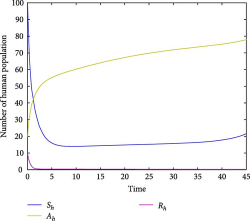
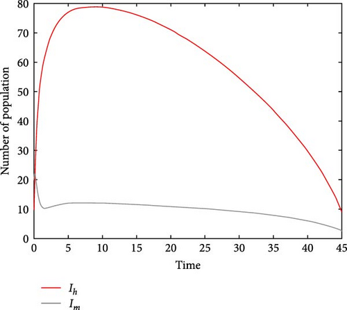
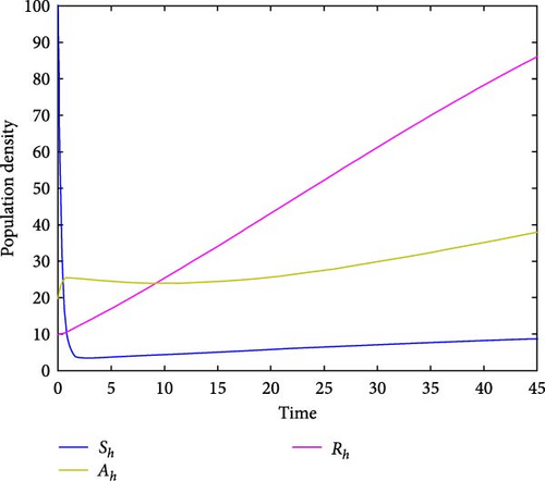
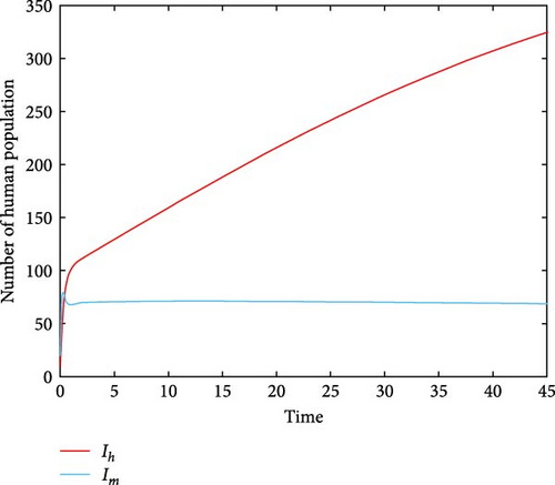
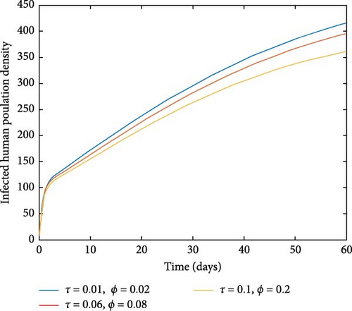
For parameter values: Λ_h = 10, β_h = 5.9, Λ_m = 500, β_m = 0.955, σ = 0.051, μ = 0.05, α = 1/15, γ = 0.00991, ω = 1.9, τ = 0.2, δ = 9.91, ϕ = 1.89, π = 0.28, the numerical simulation of model system (1) is illustrated. Figures 2(a) and 2(b) show for R₀ = 0.3812, the class of aware population A_h(t) and susceptibles populations S_h(t) are increasing, while recovered populations are decreasing. At the same condition, infected human and vector populations are decreasing but not sufficient to eradicate malaria disease. This finding supports the analytical result that the DFE point is locally asymptotically stable for R₀ < 1 as stated in Theorem 1. This result indicates that malaria disease will gradually decrease or eliminate from the population. Figures 3(a) and 3(b) shows that all solution curves approaches almost to non-zero components or to their endemic equilibrium point components for parameter values Λ_h = 10, β_h = 5.99, Λ_v = 600, β_v = 9.05, σ = 0.051, μ = 0.05, α = 1, γ = 0.01991, ω = 0.0075, τ = 0.1892, δ = 11.99, ϕ = 1.89, π = 0.18. This result revealed that the global asymptotic stability of the malaria disease persistent equilibrium point, which occurs when R₀ = 2.9713 > 1, indicates that the disease will persist in the population.

The simulation of sensitivity analysis is displayed in Figure 4(a). The baseline parameter values with positive index will result a major effect on the frequency of the ailment spread, while parameters with negative index help to reduce the disease. In Figure 4(b), for R₀ < 1, the model system (1) has stable DFE, and it has no endemic equilibrium point. While for R₀ > 1, a stable endemic equilibrium appeared, and a stable disease-free became unstable. Hence, the transcritical bifurcation arises.

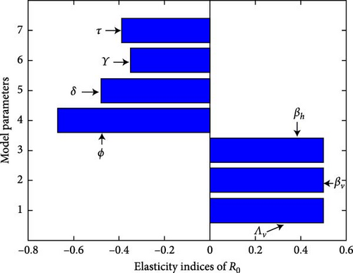
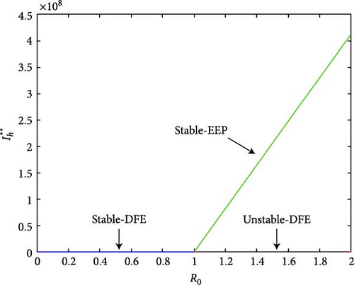
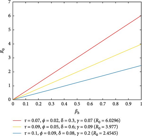
Figure 5(a) depicts that a large value of τ or γ or δ or ϕ in the presence of β_h can lead to a small value of R₀. That is to say, if we increase the awareness creation, recovery rate of infected individuals and environmental cleaning (chemical spraying), the spread of malaria disease will decrease in the population. Figure 5(b) reflects that a large value of τ or ϕ leads to a small value of R₀. Therefore, by increasing public awareness creation and chemical spraying, we can reduce the spread of malaria disease.

6.1. Numerical Results of the Optimal Control Model

In this section, we examine the effects of various control measures on the eradication of malaria disease through some numerical results.

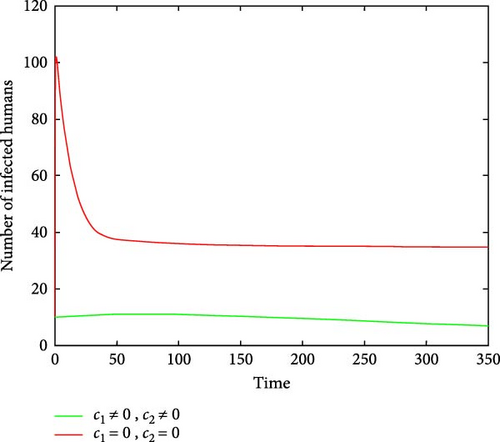
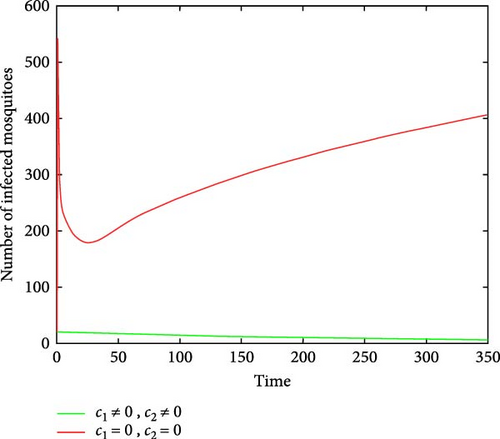
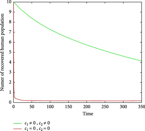
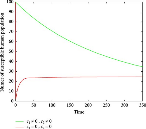
Figures 6(a) and 6(b) show the effectiveness of public awareness in the reduction of both infected human and mosquitoes population. As we observed, in the absence of a public awareness campaign, the number of infected mosquitoes increases and, in turn, this leads to an increase in the numbers of the infected human population, while in the presence of a public awareness campaign, the numbers of infected mosquitoes dramatically decrease and also infected human populations decrease at the same time. Therefore, in order to stop the spread of malaria, policymakers must focus on raising public awareness to the fullest extent possible and ensuring that there are enough preventive controls available. Figures 7(a) and 7(b) show that the number of recovered human populations is higher under the control strategy than in the case without control, while the number of susceptible mosquito populations is lower under the control strategy than in the case without control. Therefore, in order to stop the spread of malaria in the community, policymakers and the government must place a high priority on providing ongoing treatment for those who are infected.

7. Conclusion

In this study, a nonlinear deterministic mathematical model of malaria transmission is formulated and analyzed, dividing susceptible into another aware human population. Under the given domain, the mathematical as well as epidemiological welposedness of the model is proved. Malaria disease reproduction number (threshold) of the model was obtained and provided the scenarios to stick or eradicate in the population. The stability of the disease-free and endemic equilibrium points was examined, and the DFE point was found to be asymptotically stable when R₀ < 1 and the existence of bifurcation at R₀ = 1 was analyzed, and it was shown that when R₀ = 1 the model undergo forward bifurcation phenomenon. We found that R₀ < 1 is the sufficient condition to eradicate malaria disease.

The sensitivity analysis of the basic reproduction number of the model revealed that parameters with negative indices are likely to decrease the disease while parameters with positive indices are likely to increase the expansion of malaria disease in the society. The numerical simulation of the model revealed that the numbers of infected human populations decrease when the biting rate of susceptible humans by infected mosquitoes decrease. The qualitative study proved the existence and characterization of an optimal control solution. Also, various control strategies were tested and showed that the combination of continuous public awareness creation and access to adequate control measures are more effective in the control of malaria disease transmission.

Conflicts of Interest

The authors declare that they have no conflicts of interest.

Acknowledgments

The authors would like to thank Hawassa University for its Wi-Fi contribution.

Open Research

Data Availability

The data used to supplement the findings of this study are from previously published articles and cited in relevant places.

References

1 Workie Z. A. and Koya P. R., Mathematical modelling of the co-infection dynamics of typhoid fever with plasmodium vivax and plasmodium falciparum with treatment, Mathematical Modelling and Applications. (2022) 7, no. 1, 1–25.
Google Scholar
2 Huo H.-F. and Qiu G.-M., Stability of a mathematical model of malaria transmission with relapse, Abstract and Applied Analysis. (2014) 2014, 9, https://doi.org/10.1155/2014/289349, 2-s2.0-84896481687, 289349.
10.1155/2014/289349
Google Scholar
3 WHO, Malaria report, 2015, http://www.who.int/malaria/publications/world-malaria-report-2015/report/en/.
Google Scholar
4 Bakary T., Boureima S., and Sado T., A mathematical model of malaria transmission in a periodic environment, Journal of Biological Dynamics. (2018) 12, no. 1, 400–432, https://doi.org/10.1080/17513758.2018.1468935, 2-s2.0-85049215444.
10.1080/17513758.2018.1468935
PubMed Web of Science® Google Scholar
5 Mohammed H. I., Mukhtar I. M., and Sadiq H. A., Malaria and typhoid fever: prevalence, co-infection and socio-demographic determinants among pregnant women attending antenatal care at a primary healthcare facility in central Nigeria, International Journal of Pathogen Research. (2020) 5, no. 4, 17–24, https://doi.org/10.9734/ijpr/2020/v5i430140.
10.9734/ijpr/2020/v5i430140
Google Scholar
6 Tabo Z., Luboobi L. S., and Ssebuliba J., Mathematical modelling of the in-host dynamics of malaria and the effects of treatment, Journal of Mathematics and Computer Science. (2017) 17, no. 1, 1–21, https://doi.org/10.22436/jmcs.
10.22436/jmcs.017.01.01
Google Scholar
7 Wedajo A. J., Bole B. K., and Koya P. R., Analysis of SIR mathematical model for malaria disease with the inclusion of infected immigrants, IOSR Journal of Mathematics. (2018) 14, 10–21.
Google Scholar
8 WHO, World malaria day, report of the World Health Organisation, 2021, http://www.who.int/malaria/media/worldmalaria-day-2021/en/.
Google Scholar
9 Okosun K. O., Rachid O., and Marcus N., Optimal control strategies and cost-effectiveness analysis of a malaria model, Biosystems. (2013) 111, no. 2, 83–101, https://doi.org/10.1016/j.biosystems.2012.09.008, 2-s2.0-84872670823.
10.1016/j.biosystems.2012.09.008
PubMed Web of Science® Google Scholar
10 Anteneh A. A., Bazezew Y. M., and Palanisamy S., Mathematical model and analysis on the impact of awareness campaign and asymptomatic human immigrants in the transmission of COVID-19, BioMed Research International. (2022) 2022, 13, https://doi.org/10.1155/2022/6260262, 6260262.
10.1155/2022/6260262
PubMed Web of Science® Google Scholar
11 Sweileh W. M., Global research activity on mathematical modeling of transmission and control of 23 selected infectious disease outbreak, Globalization and Health. (2022) 18, https://doi.org/10.1186/s12992-022-00803-x, 4.
10.1186/s12992-022-00803-x
PubMed Google Scholar
12 Ngonghala C. N., Iboi E., Eikenberry S., Scotch M., MacIntyre C. R., Bonds M. H., and Gumel A. B., Mathematical assessment of the impact of non-pharmaceutical interventions on curtailing the 2019 novel Coronavirus, Mathematical Biosciences. (2020) 325, https://doi.org/10.1016/j.mbs.2020.108364, 108364.
10.1016/j.mbs.2020.108364
CAS PubMed Web of Science® Google Scholar
13 Ayalew A., Molla Y., Tilahun T., and Tesfa T., Mathematical model and analysis on the impacts of vaccination and treatment in the control of the COVID-19 pandemic with optimal control, Journal of Applied Mathematics. (2023) 2023, 15, https://doi.org/10.1155/2023/8570311, 8570311.
10.1155/2023/8570311
Google Scholar
14 Ozair M., Lashari A. A., Jung I. H., and Okosun K. O., Stability analysis and optimal control of a vector-borne disease with nonlinear incidence, Discrete Dynamics in Nature and Society. (2012) 2012, 21, https://doi.org/10.1155/2012/595487, 2-s2.0-84870030340, 595487.
10.1155/2012/595487
Web of Science® Google Scholar
15 Mekonen K. G. and Obsu L. L., Mathematical modeling and analysis for the co-infection of COVID-19 and tuberculosis, Heliyon. (2022) 8, no. 10, https://doi.org/10.1016/j.heliyon.2022.e11195, e11195.
10.1016/j.heliyon.2022.e11195
PubMed Web of Science® Google Scholar
16 Khan A., Zarin R., Khan S., Saeed A., Gul T., and Humphries U. W., Fractional dynamics and stability analysis of COVID-19 pandemic model under the harmonic mean type incidence rate, Computer Methods in Biomechanics and Biomedical Engineering. (2022) 25, no. 6, 619–640, https://doi.org/10.1080/10255842.2021.1972096.
10.1080/10255842.2021.1972096
PubMed Web of Science® Google Scholar
17 Ghosh M., Olaniyi S., and Obabiyi O. S., Mathematical analysis of reinfection and relapse in malaria dynamics, Applied Mathematics and Computation. (2020) 373, https://doi.org/10.1016/j.amc.2020.125044, 125044.
10.1016/j.amc.2020.125044
Google Scholar
18 Hattaf K., A new generalized definition of fractional derivative with nonsingular kernel, Computation. (2020) 8, no. 2, https://doi.org/10.3390/computation8020049, 49.
10.3390/computation8020049
Web of Science® Google Scholar
19 Ross R., The Prevention of Malaria, 1911, John Murray, London.
Google Scholar
20 Collins O. C. and Duffy K. J., A mathematical model for the dynamics and control of malaria in Nigeria, Infectious Disease Modelling. (2022) 7, no. 4, 728–741, https://doi.org/10.1016/j.idm.2022.10.005.
10.1016/j.idm.2022.10.005
CAS PubMed Google Scholar
21 Keno T. D., Makinde O. D., and Obsu L. L., Optimal control and cost effectiveness analysis of SIRS malaria disease model with temperature variability factor, Journal of Mathematical and Fundamental Sciences. (2021) 53, no. 1, 134–163, https://doi.org/10.5614/j.math.fund.sci.2021.53.1.10.
10.5614/j.math.fund.sci.2021.53.1.10
Google Scholar
22 Romero-Leiton J. P., Montoya J., and Ibargüen-Mondragón E., An optimal control problem applied to malaria disease in Colombia, Applied Mathematical Sciences. (2018) 12, no. 6, 279–292.
10.12988/ams.2018.819
Google Scholar
23 Keno T. D., Dano L. B., and Makinde O. D., Modeling and optimal control analysis for malaria transmission with role of climate variability, Computational and Mathematical Methods. (2022) 2022, 18, https://doi.org/10.1155/2022/9667396, 9667396.
10.1155/2022/9667396
Google Scholar
24 Gautam R., Pokharel A., Adhikari K., Uprety K. N., and Vaidya N. K., Modeling malaria transmission in Nepal: impact of imported cases through cross-border mobility, Journal of Biological Dynamics. (2022) 16, no. 1, 528–564, https://doi.org/10.1080/17513758.2022.2096935.
10.1080/17513758.2022.2096935
PubMed Google Scholar
25 Tilahun M., Backward bifurcation in SIRS malaria model, 2017, https://doi.org/10.48550/arXiv.1707.00924.
10.48550/arXiv.1707.00924
Google Scholar
26 Schroers B. J., Ordinary Differential Equations: A Practical Guide, 2011, Cambridge University Press.
10.1017/CBO9781139057707
Google Scholar
27 Van den Driessche P. and Watmough J., F. Brauer, P. van den Driessche, and J. Wu, Further notes on the basic reproduction number, Mathematical Epidemiology, 2008, Springer, Berlin, Heidelberg, 159–178, https://doi.org/10.1007/978-3-540-78911-6_6, 2-s2.0-42249085379.
10.1007/978-3-540-78911-6_6
Google Scholar
28 Diekmann O., Heesterbeek J. A., and Metz J. A., On the definition and the computation of the basic reproduction ratio R₀ in models for infectious diseases in heterogeneous populations, Journal of Mathematical Biology. (1990) 28, 365–382, https://doi.org/10.1007/BF00178324, 2-s2.0-0025159677.
10.1007/BF00178324
CAS PubMed Web of Science® Google Scholar
29 Lasalle J. P., The Stability of Dynamical Systems, 1976, SIAM.
10.1137/1.9781611970432
Google Scholar
30 Li Y. and Muldowney J. S., On bendixson’s criterion, Journal of Differential Equations. (1993) 106, no. 1, 27–39, https://doi.org/10.1006/jdeq.1993.1097, 2-s2.0-0002153279.
10.1006/jdeq.1993.1097
Web of Science® Google Scholar
31 Castillo-Chavez C. and Song B., Dynamical models of tuberculosis and their applications, Mathematical Biosciences and Engineering. (2004) 1, no. 2, 361–404, https://doi.org/10.3934/mbe.2004.1.361.
10.3934/mbe.2004.1.361
PubMed Web of Science® Google Scholar
32 Chitnis N., Hyman J. M., and Cushing J. M., Determining important parameters in the spread of malaria through the sensitivity analysis of a mathematical model, Bulletin of Mathematical Biology. (2008) 70, no. 5, 1272–1296, https://doi.org/10.1007/s11538-008-9299-0, 2-s2.0-47349102730.
10.1007/s11538-008-9299-0
PubMed Web of Science® Google Scholar
33 Pontryagin L. S., The Mathematical Theory of Optimal Processes, 1986, 4, 1st edition, CRC Press, New York, NY, USA.
Google Scholar
34 Pantha B., Agusto F. B., and Elmojtaba I. M., Optimal control applied to a visceral leishmaniasis model, Electronic Journal of Differential Equations. (2020) 1-132, no. 80, 1–24, https://doi.org/10.58997/ejde.2020.80.
10.58997/ejde.2020.80
Google Scholar
35 Biswas S., Subramanian A., ELMojtaba I. M., Chattopadhyay J., and Sarkar R. R., Optimal combinations of control strategies and cost-effective analysis for visceral leishmaniasis disease transmission, PLoS ONE. (2017) 12, no. 2, https://doi.org/10.1371/journal.pone.0172465, 2-s2.0-85013460598, e0172465.
10.1371/journal.pone.0172465
PubMed Web of Science® Google Scholar
36 Alzahrani E. O., Ahmad W., Altaf Khan M., and Malebary S. J., Optimal control strategies of zika virus model with mutant, Communications in Nonlinear Science and Numerical Simulation. (2021) 93, https://doi.org/10.1016/j.cnsns.2020.105532, 105532.
10.1016/j.cnsns.2020.105532
Web of Science® Google Scholar
37 Boyce W. E. and DiPrima R. C., Elementary Differential Equations and Boundary Value Problems, 2012, John Wiley and Sons, Inc.
Google Scholar
38 Pontryagin L. S., Boltyanskii V., Gamkrelidze R., and Mischchenko E., The Mathematical Theory of Optimal Processes, 1962, Interscience Publishers John Wiley & Sons, Inc., New York-London.
Web of Science® Google Scholar
39 Kar T. K. and Jana S., Application of three controls optimally in a vector-borne disease–a mathematical study, Communications in Nonlinear Science and Numerical Simulation. (2013) 18, no. 10, 2868–2884, https://doi.org/10.1016/j.cnsns.2013.01.022, 2-s2.0-84877586785.
10.1016/j.cnsns.2013.01.022
Google Scholar
40 Ibrahim M. M., Kamran M. A., Naeem Mannan M. M., Kim S., and Jung I. H., Impact of awareness to control malaria disease: a mathematical modeling approach, Complexity. (2020) 2020, 13, https://doi.org/10.1155/2020/8657410, 8657410.
10.1155/2020/8657410
Google Scholar

Citing Literature

All articles

Modeling and Stability Analysis of the Dynamics of Malaria Disease Transmission with Some Control Strategies

Abstract

1. Introduction

2. Mathematical Model Formulation and Description

3. Basic Properties of the Model

4. Analytical Analysis of the Model

4.1. Malaria Disease Free-Equilibrium (DFE) Point

4.2. Basic Reproduction Number

4.3. Malaria Disease Persistent Equilibrium Point of the Model

4.4. Stability Analysis of Model Equilibrium Points

4.5. Bifurcation Analysis of the Model

4.6. Sensitivity Analysis of the Basic Reproductive Number

4.6.1. Interpretation of Sensitivity Indices

5. Extension of the Model into Optimal Control

5.1. Existence of an Optimal Control

5.2. The Hamiltonian and Optimality System

5.3. Analysis of the Control Reproductive Number

6. Numerical Results and Discussions

6.1. Numerical Results of the Optimal Control Model

7. Conclusion

Conflicts of Interest

Acknowledgments

Open Research

Data Availability

References

Citing Literature

Figures

References

Information

About Wiley Online Library

Help & Support

Opportunities

Connect with Wiley

Modeling and Stability Analysis of the Dynamics of Malaria Disease Transmission with Some Control Strategies

Abstract

1. Introduction

2. Mathematical Model Formulation and Description

3. Basic Properties of the Model

4. Analytical Analysis of the Model

4.1. Malaria Disease Free-Equilibrium (DFE) Point

4.2. Basic Reproduction Number

4.3. Malaria Disease Persistent Equilibrium Point of the Model

4.4. Stability Analysis of Model Equilibrium Points

4.5. Bifurcation Analysis of the Model

4.6. Sensitivity Analysis of the Basic Reproductive Number

4.6.1. Interpretation of Sensitivity Indices

5. Extension of the Model into Optimal Control

5.1. Existence of an Optimal Control

5.2. The Hamiltonian and Optimality System

5.3. Analysis of the Control Reproductive Number

6. Numerical Results and Discussions

6.1. Numerical Results of the Optimal Control Model

7. Conclusion

Conflicts of Interest

Acknowledgments

Open Research

Data Availability

References

Citing Literature

Figures

References

Related

Information