Volume 2024, Issue 1 7555042

Research Article

Open Access

On a Stochastic Approach to Extensions of the Susceptible-Infected-Susceptible (SIS) Model Applied to Malaria

Abdoul Karim Drabo,

Abdoul Karim Drabo

orcid.org/0009-0000-4950-6369

Laboratoire de sciences et technologies, Université Thomas SANKARA, 12, BP, 417 Ouagadougou, Burkina Faso

Search for more papers by this author

Frédéric Bere,

Corresponding Author

Frédéric Bere

[email protected]

orcid.org/0000-0002-6864-9127

Département de mathématiques, École Normale Supérieure, 01 BP 1757, Ouagadougou 01, Burkina Faso ens-burkina.bf

Search for more papers by this author

S. P. Clovis Nitiema,

S. P. Clovis Nitiema

Laboratoire de sciences et technologies, Université Thomas SANKARA, 12, BP, 417 Ouagadougou, Burkina Faso

Département de mathématiques de décision, Université Thomas SANKARA, 12, BP, 417 Ouagadougou, Burkina Faso

Search for more papers by this author

Abdoul Karim Drabo,

Abdoul Karim Drabo

orcid.org/0009-0000-4950-6369

Laboratoire de sciences et technologies, Université Thomas SANKARA, 12, BP, 417 Ouagadougou, Burkina Faso

Search for more papers by this author

Frédéric Bere,

Corresponding Author

Frédéric Bere

[email protected]

orcid.org/0000-0002-6864-9127

Département de mathématiques, École Normale Supérieure, 01 BP 1757, Ouagadougou 01, Burkina Faso ens-burkina.bf

Search for more papers by this author

S. P. Clovis Nitiema,

S. P. Clovis Nitiema

Laboratoire de sciences et technologies, Université Thomas SANKARA, 12, BP, 417 Ouagadougou, Burkina Faso

Département de mathématiques de décision, Université Thomas SANKARA, 12, BP, 417 Ouagadougou, Burkina Faso

Search for more papers by this author

First published: 30 April 2024

https://doi.org/10.1155/2024/7555042

Citations: 1

Academic Editor: Oluwole D. Makinde

Share a link

Email
Wechat
Bluesky

Abstract

This work presents a stochastic model of malaria spread. We first calculated the basic reproduction number R₀ of the models (S_hI_hR_hS_h-S_vI_v) and (S_hL_hI_hR_hS_h-S_vL_vI_v) in order to show that the malaria-free equilibrium is asymptotically stable; then, we used a finite Markov chain model to describe the interactions between the different compartments of the model (S_eL_eI_eR_eS_e-S_aL_aI_aR_aS_a-S_vI_v). We carried out numerical simulations of our results for two types of transmission zones: a zone with low malaria transmission and an endemic zone. Through these simulations, we first determined the invariant stationary distribution π^∗ of the model, and then, we found that the use of the indoor residual spraying (IRS) method by regular application of insecticides is more effective for the elimination of malaria than the use of long-acting impregnated mosquito nets (LLINs).

1. Introduction

Mathematical models of the spread of malaria date back to the beginning of the 20th century by Ross [1]. Several mathematical models have been developed to study the dynamics of malaria spread. We can cite the models (S_hI_hS_h-S_vI_vS_v) of Ross, the models (S_hI_hR_hS_h-S_vI_v) in [2–4], and the models (S_hE_hI_hR_hS_h) in [5, 6]. The mathematical theory of the spread of malaria was solidified by Reiner et al. [7] in the 1960s. In 2018, Mbogo et al. [2] use the Galton-Watson branching processes to propose an extension of the model formulated by [4]. There are also results in the following works [8–13] that could well explain the literature. In this work, we first present in Section 2 some preliminary results, necessary for the conduct of our work by successively studying the models (S_hI_hS_h-S_vI_vS_v), (S_hI_hR_hS_h-S_vI_v), and (S_hL_hI_hR_hS_h-S_vL_vI_v). Then, we present an extension of the Markovian SIS model in a hypoendemic and endemic area in Sections 3.2 and 3.3, respectively. And finally, Section 4 is devoted to the work of numerical simulations of our results.

2. Mathematical Preliminaries and Notations

2.1. Ross’s (S_hI_hS_h-S_vI_vS_v) Model

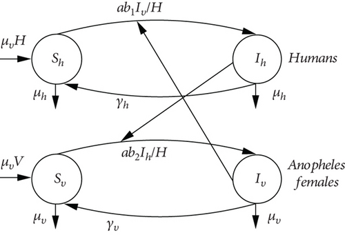
In 1911, Sir Ronald Ross proposed a model which took into account both anopheline and human populations. This model is certainly the starting point for vector-host models. Ross divided hosts (humans) and vectors (anopheles) into two classes, susceptible and infected, respectively. Let S_h be the population of susceptible humans and I_h the population of infected humans. Ross assumes that there is no latency period and that, consequently, an infected person is automatically an infectious person. Similarly, he refers to the population of susceptible anopheles as S_v and the population of infected anopheles as I_v. In his model, Ross assumes that both the human and Anopheles populations are constant and that one mosquito bites “a” humans per unit of time where “a” is constant [14]. The malaria propagation graph in Ross’s (S_hI_hS_h-S_vI_vS_v) model is shown in Figure 1.

Details are in the caption following the image — **Figure 1**
Open in figure viewer PowerPoint

The final graph of disease transmission.

He obtained the differential system (1) governing the (S_hI_hS_h-S_vI_vS_v) model of malaria.

(1)

Assuming that the human and Anopheles populations are constant, Ross used two ordinary differential equations (2) to model the evolution of the fraction of individuals in the classes of infected (I_h, I_v).

(2)

According to Ross, eradicating malaria requires reducing the number of infectious mosquitoes below a certain threshold. He determines the basic reproduction number R₀ per

(3)

and formulates the following corollary [15, 16].

Corollary 1.

(1)
If R₀ ≤ 1, then the disease completely disappears from the population after a certain time
(2)
If R₀ > 1, then the disease remains endemic in the population.

2.2. Model (S_hI_hR_hS_h-S_vI_v)

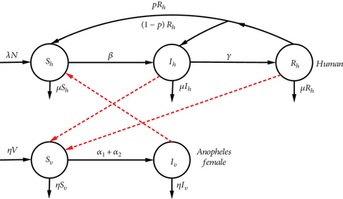
Since malaria provides temporary immunity and is not lethal if treated, it is possible to use a SIRS (Susceptible-Infected-Recovered-Susceptible) model, since recovered individuals return to the S class with probability p(p > 0) or relapsed individuals become infected again with probability 1 − p. So to Ross’s (S_hI_hS_h-S_vI_vS_v) model, we add the R recovered compartment. These types of model are also solved in [17, 18]. Figure 2 illustrates the scheme of disease progression.

In this model, the differential equation system satisfies the following equation:

(4)

where S_h, I_h, R_h, S_v, and I_v represent the number of susceptible humans, infectious humans, recovered humans, susceptible mosquitoes, and infectious mosquitoes, respectively. These types of models (S_hI_hR_hS_h-S_vI_v) are also studied by authors such as [2–4].

2.3. Model (S_hL_hI_hR_hS_h-S_vL_vI_v)

According to the literature, the average delay between exposure to parasitised blood and the first clinical signs of infection is 4 to 17 days for P. falciparum. There is therefore an additional class of exposed individuals (E) or latent individuals (L) who are not yet infectious. It is therefore necessary to model the dynamics of the spread of malaria using the (S_hL_hI_hR_hS_h-S_vL_vI_v) model, which would be an extension of the (S_hI_hS_h-S_vI_vS_v) and (S_hI_hR_hS_h-S_vI_v) models previously studied. The disease progression diagram in this type of model can be represented in Figure 3.

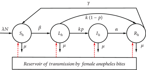
The ordinary differential equations (ODEs) governing the deterministic SLIRS model are presented by the system of

(5)

Mosquito ODEs are neglected for simplicity. All parameters and their biological interpretation are recorded in Table 1.

Table 1. Model parameters and their meanings.

Parameter	Biological interpretation
N	Size of the human population (N = S + L + I + R)
λ	Birth rate
μ	Death rate
k	Incubation rate
p	Probability of transition from latent to infectious state
1 − p	Probability of transition from latent to recovered state
β	Transmission rate (susceptible to latent)
α	Transmission rate (infectious to removed)
γ	Immunity loss rate (removed to susceptible)

Once we know the triplet (S, L, I), we can work with the reduced system (6) and then deduce R because N = S + L + I + R.

(6)

The disease-free equilibrium (DFE) of this model is therefore (N, 0, 0). Authors such as [17, 19, 20] have also studied these types of models.

3. Main Results

3.1. Basic Reproduction Rate R₀

Theorem 2. The basic reproduction rates R₀ of the models (S_hI_hR_hS_h-S_vI_v) in Section 2.2 and (S_hL_hI_hR_hS_h-S_vL_vI_v) in Section 2.3 are given by

(7)

Proof. To determine the basic reproduction rate R₀, we apply the Van den Driessche method [15]. The nonlinear ordinary differential equation system (4) integrating the compartments of the model in Figure 2 can be expressed as

(8)

where

represents new infections and

represents the rate of individuals entering and exiting the j compartment, respectively [15]. The Jacobian matrices of

and

at equilibrium without disease E₀ are

(9)

The inverse matrix of V is

(10)

with

(11)

The set of eigenvalues of FV⁻¹ is denoted Sp(FV⁻¹) and is equal

(12)

The basic reproduction number R₀ is the spectral radius of the next generation matrix:

(13)

The basic reproduction number R₀₁ of our model (4) in Section 2.2 is

(14)

Similarly for the model (6) in Section 2.3, we have

(15)

Hence,

(16)

Therefore,

(17)

Then, the basic reproduction rate R₀₂ is given by the spectral radius of FV⁻¹.

Corollary 3. The disease-free equilibrium of the system (6) is locally and asymptotically stable if R₀₁ < 1 and unstable if R₀₁ > 1.

Corollary 4. The malaria-free equilibrium E₀ of the system (4) is locally asymptotically stable if R₀₂ < 1 and unstable if R₀₂ > 1.

3.2. Extension of the Markov SIS Model in a Hypoendemic Zone

In this section, we develop a stochastic model for malaria transmission by considering two types of host (“nonimmune” and “semi-immune”) in the human population. The “nonimmune” group comprises human individuals who have never acquired any immunity to malaria. It is assumed that these hosts are vulnerable because they can suffer and/or die from malaria. “Semi-immune” people are those who have acquired or lost at least some immunity to malaria in their lifetime. It is assumed that these hosts are nonvulnerable, so they cannot die from malaria but can only suffer from it. We envisage a model of the type (S_eL_eI_eR_eS_e) for nonimmunes until they enter the semi-immune category and then follow a model of the type (S_aL_aI_aR_aS_a), where e and a denote the index for nonimmunes and semi-immunes, respectively. For the mosquito population, we use a model of the type (S_vI_v).

3.2.1. Elaboration of the Model

We consider that it is the gametocyte form of Plasmodium in humans that transmits the infection to mosquitoes and the sporozoite form in the mosquito that transmits the infection to humans. In our model, we adopt a number of operational definitions.

(1) Terminology.

(i)
Susceptible (S): an individual bitten by infectious mosquitoes and capable of contracting malaria
(ii)
Latent (L): individual who has contracted malaria but does not transmit it initially
(iii)
Infectious (I): an individual who harbours a high level of parasites in gametocyte form. They can suffer and/or die from malaria
(iv)
Immune (R): an asymptomatic carrier of the parasite. This is a state of protection against the disease, but not against the parasite; it is a healing stage

A human being is said to be ill with malaria if he or she is either in a latent or infectious state. In order to write the model, the nonimmune human host types are subdivided into four (4) compartments: susceptible (S_e), latent (L_e), infectious (I_e), and immune (R_e). Semi-immune human host types are also subdivided into four (4) compartments: susceptible (S_a), latent (L_a), infectious (I_a), and immune (R_a). The mosquito population is made up of susceptible (S_v) and infectious (I_v) mosquitoes. We are studying two heterogeneous populations made up of several pathological classes, in which individuals can move from one class to another. There are ten different disease states. The pattern of disease progression in this model is illustrated in Figure 4.

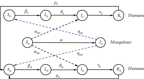
The solid arrows indicate the direction of propagation of Plasmodium, thus creating states of health in the subjects.

The red dotted arrows indicating the direction of infection from an infectious mosquito (I_v) to a nonimmune susceptible human individual (S_e) or a semi-immune susceptible human individual.

The black dotted arrows indicate the direction of infection of a susceptible mosquito (S_v) on an infectious nonimmune human (I_e) or an infectious nonimmune human (I_a).

3.2.2. Model Assumptions

A1: the probabilities η_ve, η_va, α_ev, α_av, and α are in the interval [0, 1[.

A2: the parameters β_e, θ_e, η_e, ρ_e, β_a, θ_a, η_a, and ρ_a are assumed to be strictly positive in the interval ]0, 1[ and represent the probabilities of moving from a subfund i to a subfund j.

A3: these passage probabilities and parameters designate the conditional probabilities ℙ(X₁ = compartment j|X₀ = compartment i) satisfying the Markov property. These conditional probabilities linking two consecutive pathological states are between ]0, 1[ if the transition has a biological meaning and 0 otherwise.

3.2.3. Interaction between Humans and Mosquitoes

Initially, infectious mosquitoes (I_v) bite susceptible humans (S_e) with a η_ve probability. The latter may remain susceptible (S_e) with probability r for some time or become latent (L_e) with probability β_e. Individuals can remain latent for a given time with probability q or become infectious (I_e) with θ_e as the transition probability. In this infectious state (I_e), humans can die with a probability μ or become immune with a probability equal to ν_e, or even remain infectious with a probability p for an interval of time. Having completed the 1^st cycle, the immune (R_e) becomes susceptible (S_a) to the ρ_e immunity rate, and through the intermediary of the infectious mosquito (I_v), the cycle resumes as shown in Figure 4. At stage (R_a), having acquired a certain immunity, the individual re-enters the susceptible class (S_a) at the rate ρ_a. The susceptible mosquitoes (S_v) inoculate the parasite from a blood meal on the infectious (I_e) and I_a with probabilities α_ev and α_av, respectively; then, they become infectious (I_v) with probability α.

Tables 2–4 summarise the parameters that will be described in the model.

Proposition 5. Let be a probability space and X = {X_n, n ≥ 0} the process of the mode of transmission of plasmodia with values in the discrete state space . Then, the process X defined on with values in is an irreducible and aperiodic homogeneous Markov chain with initial distribution and transition matrix H, where is the probability that the process X is in state i at time 0. And this Markov chain has a stationary distribution π^∗ such that π^∗ = lim_k⟶∞π₀H^k.

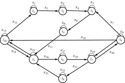
Proof. We consider that the ten compartments S_e, L_e, I_e, R_e, S_a, L_a, I_a, R_a, S_v, and I_v in Figure 4 represent the ten states of a Markov chain. These ten states are denoted {i₁, i₂, i₃, i₄, i₅, i₆, i₇, i₈, i₉, i₁₀}, respectively. Let be the set of ten states of the Markov chain. Let X = {X_n, n ≥ 0} be the process of the mode of transmission and evolution of Plasmodium. Let denote the probability that the process is in state j at time n + 1 knowing that it is in state i at time n. Furthermore, the probability is assumed to be independent of n. For all , p_ij is called the transition probability from state i to state j. The probabilistic transition graph of the Markov chain model is given in Figure 5, where the x_i, i ∈ {1, ⋯, 23} correspond to the different parameters of the model and represent the transition probabilities of the chain. The chain is irreducible because its representative graph (Figure 5) is strongly connected.

Table 2. Plasmodium transmission parameters for the nonimmune host type.

Param.	Meaning	Unity
β_e	Rate of transition from the susceptible state S_e to the latent state L_e.	Without Dim.
θ_e	Rate of transition from latent state L_e to infectious state I_e.	Without Dim.
ν_e	Rate of transition from infectious state I_e to immune state R_e.	Without Dim.

Table 3. Contact parameters between humans and mosquitoes and their dimensions.

Param.	Meaning	Unity
n_a	Number of times a mosquito could bite a human being per unit of time, if human beings were freely available	Time^–1
η_ev	Probability of transmission of an infection from an infectious mosquito (I_v) to a susceptible nonimmune human (S_e)	Without Dim.
η_va	Probability of transmission of an infection from an infectious mosquito (I_v) to a susceptible nonimmune human (S_a)	Without Dim.
α_ev	Probability of transmission of infection from an infectious human being (I_e) to a susceptible mosquito (S_v), given that there has been contact between the two	Without Dim.
α_av	Probability of transmission of infection from an infectious human being (I_a) to a susceptible mosquito (S_a), given that there has been contact between the two	Without Dim.

Table 4. Plasmodium transmission parameters for the semi-immune host type.

Param.	Meaning	Unity
β_a	Rate of transition from the susceptible state S_a to the latent state L_a	Without Dim.
θ_a	Rate of transition from latent state L_a to infectious state I_a	Without Dim.
ν_a	Rate of transition from infectious state I_a to immune state R_a	Without Dim.
ρ_e	Rate of transition from the immune state R_e to the susceptible state S_a	Without Dim.
ρ_a	Rate of transition from the immune state R_a to the susceptible state S_a	Without Dim.

Under hypothesis A3, the p_ij are grouped together in a matrix H defined by the relation

(18)

The H matrix thus constructed is stochastic by extension of the SIS model.

Furthermore, during the clinical manifestations of malaria, the future state of the patient does not depend on the previous state, but rather on the current state (the system has no “memory”). All the information needed to predict the future is contained in the current state of the process. So we can say that the spread and evolution of malaria satisfy the weak Markov property (discrete time, discrete space): for any n ≥ 0, for any sequence of states

(19)

as soon as ℙ(X₀ = i₀, X₁ = i₁, ⋯, X_n−1 = i_n−1, X_n = i) > 0. This property expresses the fact that the law of X_n+1 depends on X₀, ⋯, X_n only through the value of X_n: the “present” (X_n) gives as much information about the “future” (X_n+1) as if we knew all the “past” X₀, ⋯, X_n. By hypothesis, the transition mechanism does not change over time. The weak Markov property then takes the following form:

(20)

i.e.,

(21)

which expresses the homogeneity of the process in time.

3.3. Extending the SIS Markov Model to an Endemic Area

Children under 5 years old are the most vulnerable to malaria in endemic areas [21–24]. They have not yet developed their own immunity and are therefore considered nonimmune. We do not take into account the age of the individual but rather his or her immunological status, because according to studies [25, 26], children and adults have the same probability of being infected by malaria. It is assumed that there has been one case of death in the infectious nonimmune human compartments. Then, the Plasmodium propagation diagram takes the form of Figure 6.

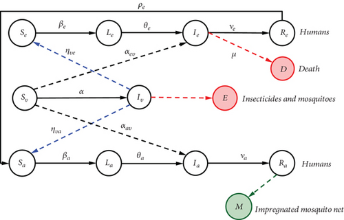
The solid arrows indicate the direction of propagation of Plasmodium, thus creating states of health in the subjects.

The blue dotted arrows indicate the direction of infection from an infectious mosquito (I_v) to a nonimmune susceptible human individual (S_e) or a semi-immune susceptible human individual.

The black dotted arrows indicate the direction of infection of a susceptible mosquito (S_v) on an infectious nonimmune human (I_e) or an infectious nonimmune human (I_a).

The red dotted arrows indicate a case of death:

(i)
of infectious nonimmune human (I_e) thus entering compartment D, where μ represents the probability of dying from malaria knowing that the nonimmune human is infectious
(ii)
mosquitoes by intradomiciliary spraying

The green dotted arrow indicates the use of long-lasting impregnated mosquito nets.

3.3.1. Model Assumptions

We supplement the list of assumptions in the previous Section 3.2 with two more:

A4: infectious mosquitoes I_v are eliminated by intradomiciliary insecticide spraying with a probability p, (p ∈ ]0, 1[).

A5: humans use long-acting impregnated mosquito nets with a probability of 1 − p, and for reasons of model simplification, environmental factors that could have more or less significant effects are neglected.

Proposition 6. Let be a probability space and X = {X_n, n ≥ 0} the process of the mode of transmission of plasmodia with values in the discrete state space . Then, the process X defined on with values in E is a homogeneous absorbing Markov chain with transition matrix P.

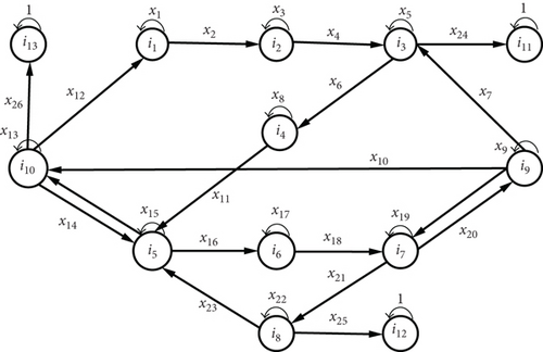
Proof. The graph representing the Markov chain model is given in Figure 7, where the x_i, i ∈ {1, ⋯, 26} correspond to the different parameters of the model and represent the transition probabilities of the chain.

There are three absorbing states (i₁₁, i₁₂, i₁₃) on the graph. As a result, the chain is absorbent. And under the assumptions A1,…,A5 and under the same interactions between humans and mosquitoes described in the previous section, we group the p_ij in a matrix P whose canonical form is represented by the relation

(22)

The matrix of transient states Q and that of absorbing states R are given by the relations

(23)

(24)

The fundamental matrix will be determined by application.

Proposition 7. The matrix elements n_i,j≔(I − Q)_i,j give us the expectation of the total number N_i(j) of stays in j before passing beyond the transient states, and the i line of (I − Q)⁻¹ gives us the “expected life balance,” with a given initial state i.

Proof. Let I_k be the indicator of being present in the transient state at time k. We pose

(25)

We have

. Considering also the breakdown into indicators

(26)

where I_k,j is the indicator of being in position

at time k. As a result,

(27)

By changing the order of summation, we obtain

(28)

where n_i,j = (I − Q)_i,j is the total expected time spent in j starting from state i.

4. Numerical Simulations

4.1. Values Assigned to Transition Probabilities

In this section, we numerically analyse the stochastic matrices (18) and (22). We consider two malaria transmission zones: zone A corresponding to a low transmission zone and zone B corresponding to a high transmission zone. We begin by determining the values of the biological parameters equivalent to the transition probabilities in each zone. Most of these data are obtained from the literature, in particular from models developed by [27–31].

4.1.1. The Transition Probabilities between the Three Types of Host

The probability of effective transition between the three host types is the average number of contacts per unit of time (in this case the day) that could lead to infection of a specific host type.

n_a: we estimate that the average number of mosquito bites a human being can suffer per day is 0.28 for the low transmission zone and 0.38 for the high transmission zone. This average number n_a is a function of the exposed surface area of the human and any vector control interventions used by humans to reduce exposure to mosquitoes [27, 30].

η_ve: we estimate that the probability of transmission of an infection from an infectious mosquito (I_v) to a susceptible nonimmune human being (S_e), knowing that there has been contact between the two, is 0.021 for the low transmission zone and 0.07 for the high transmission zone [30].

η_va: we estimate that the probability of transmission of an infection from an infectious mosquito (I_v) to a susceptible semi-immune human being (S_a), knowing that there has been contact between the two, is 0.012 for the low transmission zone and 0.022 for the high transmission zone [28, 31].

α_ev: we assume that the probability of transmission of infection from an infectious nonimmune human being (I_e) to a susceptible mosquito (S_v), given that there has been contact between the two, is 0.11 for a low transmission zone and 0.45 for a high transmission zone [31].

α_av: we assume that the probability of transmission of infection from an infectious semi-immune human being (I_a) to a susceptible mosquito (S_v), given that there has been contact between the two, is 0.08 for an area of low transmission and 0.35 for an area of high transmission.

4.1.2. Transitions in Nonimmune Host Compartments

β_e: the probability of transition from the susceptible state (S_e) to the latent state (L_e). This parameter results from the infection force which is defined by

(29)

where N_h is the human population size and N_v is the mosquito population size [28–30].

θ_e: the probability of transition from the latent state (L_e) to the infectious state (I_e). We assume that θ_e = 0.10 for both types of zone.

ν_e: the probability of transition from the infectious state (I_e) to the immune state (R_e). We have assumed that this rate is 0.005 for the zone of low transmission and 0.001 for the zone of high transmission zone.

ρ_e: the probability of transition from the immune state (R_e) to the susceptible state (S_a). This is a phase of change of status from nonimmune to semi-immune hosts. We have assumed that this probability is 5.5 × 10⁻⁴ for the low transmission zone and 2.7 × 10⁻³ for the high transmission zone [27, 29, 31].

4.1.3. Transitions in the Compartments of Semi-immune Hosts

β_a: the probability of transition from the susceptible state (S_a) to the latent state (L_a). This parameter results from the strength of infection of the semi-immunes, which is defined by

(30)

where N_h is the size of the human population and N_v is the size of the mosquito population [28–30].

θ_a: the probability of transition from the latent state (L_a) to the infectious state (I_a). We assume that θ_a = 0.09 for both types of zone.

ν_a: the probability of transition from the infectious state (I_a) to the immune state (R_a). We have assumed that this rate is 0.01 for both types of zone.

ρ_a: the probability of transition from the immune state (R_a) to the susceptible state (S_a). Here, the immune cells heal and return to the susceptible compartment. We assume that ρ_a = 0.0083 for the low transmission zone and ρ_a = 0.033 for the high transmission zone [30].

For i = j, the p_ii are obtained by stochastic effect. The other transition probabilities not quoted here are obtained by using the Markov property.

All these estimated probabilities are summarised in Table 5.

Table 5. Transition probabilities in zones A and B.

Param.	Zone A	Zone B	Intervals
n_a	0.25	0.38	0.13-0.47
η_ve	0.021	0.07	0.01-0.27
η_va	0.012	0.022	0.01-0.27
α_ev	0.11	0.45	0.072-0.64
α_va	0.08	0.35	0.072-0.64
θ_e	0.10	0.10	0.067-0.20
θ_a	0.09	0.09	0.067-0.20
ν_e	0.005	0.001	0.0014-0.017
ν_a	0.01	0.01	0.0014-0.017
ρ_e	5.5 × 10⁻⁴	2.7 × 10⁻³	1.1 × 10⁻² − 5.5 × 10⁻⁵

4.2. Study of the H Matrix in a Zone A

In this section, we numerically analyse the H matrices derived from the relationship (18) using the parameter values obtained in Table 5 (zone A), which correspond to a stable transmission zone. We obtain the H matrix of the relationship (31) with values in [0, 1[.

(31)

We consider a heterogeneous population of humans and mosquitoes made up of eighty people and twenty mosquitoes assumed to be under normal conditions of temperature and reproduction. The human population is made up of fifty-seven nonimmune host types and twenty-three semi-immune host types. This gives the initial distribution given by the relationship

(32)

that is, 20% of susceptible nonimmune, 15% of latent nonimmune, 10% of infectious nonimmune, 12% of recovered nonimmune, 9% of susceptible mosquitoes, 11% of infectious mosquitoes, 5% of susceptible semi-immune, 8% of latent semi-immune, 6% of infectious semi-immune, and 4% of recovered semi-immune. We use R version 4.2.1 (2022-06-23 ucrt)-“Funny-Looking Kid” for the simulation results. Tables 6 and 7 give the probabilities π_n = π₀Hⁿ for n = {1, 2, ⋯, 21}. They illustrate the evolution of the different stages of malaria over a period of twenty-one malaria episodes, using the initial distribution π₀ of the relationship (32).

Table 6. The state of the probability of individuals after twenty-one episodes for an initial vector π₀ given by

	1	2	3	4	5	6	7	8	9	10
S_e	0.167	0.138	0.114	0.095	0.081	0.072	0.067	0.064	0.063	0.064
L_e	0.118	0.093	0.074	0.059	0.047	0.039	0.032	0.028	0.024	0.022
I_e	0.121	0.127	0.125	0.119	0.110	0.102	0.094	0.088	0.083	0.080
R_e	0.118	0.117	0.116	0.115	0.113	0.110	0.106	0.102	0.099	0.095
S_v	0.087	0.098	0.116	0.137	0.158	0.177	0.193	0.207	0.218	0.226
I_v	0.085	0.070	0.063	0.062	0.065	0.070	0.076	0.082	0.087	0.092
S_a	0.044	0.039	0.036	0.033	0.030	0.028	0.027	0.026	0.025	0.024
L_a	0.099	0.112	0.122	0.129	0.133	0.135	0.136	0.136	0.136	0.135
I_a	0.121	0.162	0.188	0.205	0.214	0.219	0.220	0.219	0.218	0.216
R_a	0.042	0.044	0.046	0.047	0.048	0.048	0.048	0.048	0.047	0.047

Table 7. The state of the probability of individuals after twenty-one episodes for an initial vector π₀ given by π₀ = (0.200, 0.150, 0.100, 0.120, 0.090, 0.110, 0.050, 0.080, 0.060, 0.040).

	11	12	13	14	15	16	17	18	19	20	21
S_e	0.065	0.067	0.069	0.071	0.072	0.074	0.075	0.076	0.077	0.078	0.078
L_e	0.021	0.020	0.019	0.019	0.019	0.019	0.019	0.019	0.020	0.020	0.020
I_e	0.077	0.076	0.075	0.075	0.076	0.076	0.077	0.078	0.078	0.079	0.079
R_e	0.091	0.088	0.085	0.082	0.080	0.078	0.077	0.076	0.075	0.074	0.074
S_v	0.233	0.238	0.241	0.243	0.245	0.246	0.246	0.247	0.247	0.247	0.247
I_v	0.096	0.099	0.101	0.103	0.104	0.105	0.106	0.106	0.107	0.107	0.107
S_a	0.023	0.023	0.023	0.022	0.022	0.022	0.220	0.022	0.022	0.022	0.022
L_a	0.134	0.133	0.132	0.130	0.130	0.129	0.128	0.127	0.127	0.126	0.126
I_a	0.214	0.212	0.210	0.209	0.208	0.207	0.206	0.205	0.205	0.205	0.205
R_a	0.046	0.045	0.045	0.044	0.044	0.044	0.044	0.043	0.043	0.043	0.043

The stationary distribution obtained is π^∗ and is given by the relation

(33)

Graphical representations of the results of Tables 6 and 7 are listed in Figure 8.

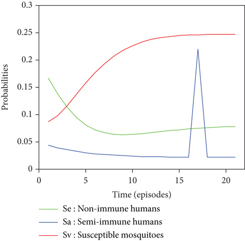
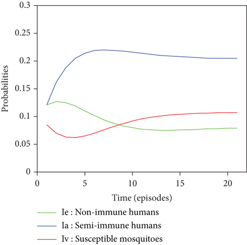
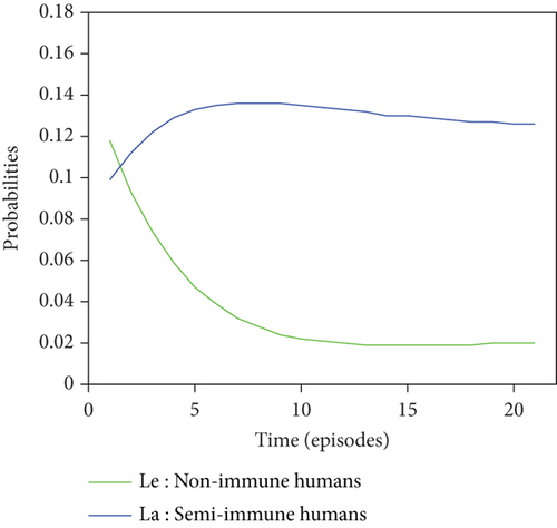
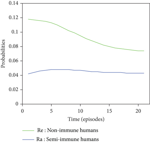
For a given initial distribution, the population of susceptible Anopheles mosquitoes increases and stabilises at around 25%. There has also been an increase in the number of infectious mosquitoes. The rapid decline in the susceptible nonimmune curve led to rapid growth in the susceptible semi-immune curve, creating a peak of probability 0.22 which stabilised after the twentieth episode. After several episodes of malaria, nonimmune individuals gradually migrate to the semi-immune class to acquire a certain level of immunity, leading to a high level of semi-immune individuals, which stabilises from the twentieth episode onwards.

4.3. Study of the P Matrix in an Endemic Area

Using the parameters obtained in Table 5 (zone B), we obtain the numerical values of the absorbing matrix P of the relation (22) described by the relation

(34)

The matrix of transient states Q and that of absorbing states R of the matrix P are given in the following the relations.

(35)

(36)

4.3.1. Fundamental Matrix

The fundamental matrix of an absorbing Markov chain can be used to extract many properties of this chain. In particular, it can be used to determine the average number of visits to a given state before absorption, the time expectancy until absorption starting from a given state, and the probabilities of being absorbed in a given state k, starting from a state i. The fundamental matrix resulting from the P matrix is given by the relation

(37)

Thus, for an individual in the state S_e, the average number of months before absorption by D or M is 1.163 ≈ 35 days in S_e, 0.047 ≈ 2 days in L_e, 0.142 ≈ 4 days in I_e, 0.475 ≈ 14 days in L_a, and 0.757 in I_a. For infectious mosquitoes I_e, the average number of months before absorption by E (eliminated by insecticides) or M (eliminated by LLINs) is 0.261 ≈ 7 days in S_e, 0.052 ≈ 2 days in L_e, and 0.156 ≈ 5 days in I_e. With absorbing Markov chains, all equilibrium distributions will be limited to state absorbents, here D, E, and M. Also, we can determine the probabilities of absorption of states S_e to R_a by states D, E, and M. To do this, let us consider the matrix B = NR defined by the relation

(38)

According to these results, the probability of an individual S_e, L_e, I_e, R_e, S_a, L_a, I_a, and R_a dying from malaria is equal to 0.006, 0.006, 0.046, 0.000, 0.005, 0.002, and 0.001, respectively. It can be seen that the probability of an infectious individual I_e dying from malaria is consistent with the clinical results. Susceptible mosquitoes S_v (infectious I_v, respectively) are absorbed either by insecticides E at 95.3% (at 82.9%, respectively) or by LLINs at 04.6% (at 16.6%, respectively). The results show that to eliminate malaria, it is preferable to use indoor residual spraying (IRS) by regular application of insecticides rather than long-acting impregnated mosquito nets (LLINs). Susceptible individuals S_e and S_a are absorbed by IRS at 62.1% and 84.5% and by LLIN at 37.4% and 14.8%, respectively. This means that susceptible humans prefer IRS rather than LLINs to protect themselves against parasite infection.

5. Conclusion

In this study, we proposed a Markovian stochastic approach to a compartment model regarding malaria transmission. This Markovian model (S_eL_eI_eR_eS_e-S_aL_aI_aR_aS_a-S_vI_v) generalizes the host-vector compartment models of types (S_hI_h-S_vI_v), (S_hI_hR_hS_h-S_vI_v), and (S_hL_hI_hR_hS_h-S_vL_vI_v). The study of this model made it possible to identify a technique suitable for combating malaria. Our model constitutes a valuable tool for the stochastic modeling of epidemics: it is used to predict the evolution of the dynamics of malaria in a human and anopheline population. In the forthcoming paper, we will study the geometric V-ergodicity of the model by including the effect of abiotic factors such as temperature.

Conflicts of Interest

The authors declare that they have no conflicts of interest.

Open Research

Data Availability

All the data is in the article.

References

1 Ross R., The Prevention of Malaria, 1911, John Murray.
Google Scholar
2 Mbogo R. W., Luboobi L. S., and Odhiambo J. W., A stochastic model for malaria transmission dynamics, Journal of Applied Mathematics. (2018) 2018, 13, https://doi.org/10.1155/2018/2439520, 2439520.
10.1155/2018/2439520
Google Scholar
3 Gweryina R. I. and Kimbir A. R., Dynamical behavior of a malaria relapse model with insecticide treated nets (ITNs) as protection measure, Applications and Applied Mathematics: An International Journal (AAM). (2020) 15, no. 1.
Web of Science® Google Scholar
4 Huo H.-F. and Qiu G.-M., Stability of a mathematical model of malaria transmission with relapse, Abstract and Applied Analysis. (2014) 2014, 9, https://doi.org/10.1155/2014/289349, 2-s2.0-84896481687, 289349.
10.1155/2014/289349
Google Scholar
5 Cai Y., Kang Y., and Wang W., A stochastic SIRS epidemic model with nonlinear incidence rate, Applied Mathematics and Computation. (2017) 305, 221–240, https://doi.org/10.1016/j.amc.2017.02.003, 2-s2.0-85013657162.
10.1016/j.amc.2017.02.003
Web of Science® Google Scholar
6 Ren X. and Zhang T., Global analysis of an SEIR epidemic model with a ratio-dependent nonlinear incidence rate, Journal of Applied Mathematics and Physics. (2017) 5, no. 12, 2311–2319, https://doi.org/10.4236/jamp.2017.512188.
10.4236/jamp.2017.512188
Google Scholar
7 ReinerR. C.Jr., Perkins T. A., Barker C. M., Niu T., Chaves L. F., Ellis A. M., George D. B., Le Menach A., Pulliam J. R., Bisanzio D., and Buckee C., A systematic review of mathematical models of mosquito-borne pathogen transmission: 1970–2010, Journal of The Royal Society Interface. (2013) 10, no. 81, article 20120921, https://doi.org/10.1098/rsif.2012.0921, 2-s2.0-84875746806.
10.1098/rsif.2012.0921
PubMed Web of Science® Google Scholar
8 Arku D., Kallah-Dagadu G., and Debrah G., A stochastic H-U model for malaria transmission via Markov theory, Journal of Biostatistics. (2021) 18, no. 3, 459–473, https://doi.org/10.20944/preprints202010.0522.v1.
10.17654/BS018030459
Web of Science® Google Scholar
9 Bedi P., Kumar A., Abdeljawad T., and Khan A., Existence of mild solutions for impulsive neutral Hilfer fractional evolution equations, Advances in Difference Equations. (2020) 2020, no. 1, 16, https://doi.org/10.1186/s13662-020-02615-y.
10.1186/s13662-020-02615-y
Google Scholar
10 Khan A., Li Y., Shah K., and Khan T. S., On coupled p-laplacian fractional differential equations with nonlinear boundary conditions, Complexity. (2017) 2017, 9, https://doi.org/10.1155/2017/8197610, 2-s2.0-85028692015, 8197610.
10.1155/2017/8197610
Google Scholar
11 Begum R., Tunç O., Khan H., Gulzar H., and Khan A., A fractional order Zika virus model with Mittag–Leffler kernel, Chaos, Solitons & Fractals. (2021) 146, article 110898, https://doi.org/10.1016/j.chaos.2021.110898.
10.1016/j.chaos.2021.110898
Web of Science® Google Scholar
12 Devi A., Kumar A., Baleanu D., and Khan A., On stability analysis and existence of positive solutions for a general non-linear fractional differential equations, Advances in Difference Equations. (2020) 2020, no. 1, 16, https://doi.org/10.1186/s13662-020-02729-3.
10.1186/s13662-020-02729-3
Google Scholar
13 Devi A., Kumar A., Abdeljawad T., and Khan A., Stability analysis of solutions and existence theory of fractional Lagevin equation, Alexandria Engineering Journal. (2021) 60, no. 4, 3641–3647, https://doi.org/10.1016/j.aej.2021.02.011.
10.1016/j.aej.2021.02.011
Web of Science® Google Scholar
14 Bichara D., Study of epidemiological models: stability, observation and estimation of parameters, [Ph.D. thesis], 2013, University of Lorraine.
Google Scholar
15 Van den Driessche P. and Watmough J., Reproduction numbers and sub-threshold endemic equilibria for compartmental models of disease transmission, Mathematical Biosciences. (2002) 180, no. 1-2, 29–48, https://doi.org/10.1016/S0025-5564(02)00108-6, 2-s2.0-0036845274, 12387915.
10.1016/S0025-5564(02)00108-6
CAS PubMed Web of Science® Google Scholar
16 Ondo J. M. M., Spatial aspects in epidemiological modelling, [Ph.D. thesis], 2012, University of Grenoble.
Google Scholar
17 Banasiak J., Ouifki R., and Woldegerima W. A., Some mathematical tools for modelling malaria: a subjective survey, Biomath. (2021) 10, article 2110029.
Google Scholar
18 Mugabi F., Duffy K. J., Mugisha J. Y. T., and Collins O. C., Determining the effects of transplacental and direct transmission on the probability of persistence in a bluetongue virus model in temperate and tropical regions, Results in Applied Mathematics. (2020) 7, article 100120, https://doi.org/10.1016/j.rinam.2020.100120.
10.1016/j.rinam.2020.100120
Google Scholar
19 Khan M. A. and Atangana A., Modeling the dynamics of novel coronavirus (2019-nCov) with fractional derivative, Alexandria Engineering Journal. (2020) 59, no. 4, 2379–2389, https://doi.org/10.1016/j.aej.2020.02.033.
10.1016/j.aej.2020.02.033
Web of Science® Google Scholar
20 Atangana A. and Araz S. I., Advanced analysis in epidemiological modeling: detection of wave, 2021, medRxiv.
Google Scholar
21 Kalipeni E., Determinants of infant mortality in Malawi: a spatial perspective, Social Science & Medicine. (1993) 37, no. 2, 183–198, https://doi.org/10.1016/0277-9536(93)90454-C, 2-s2.0-0027330478, 8351533.
10.1016/0277-9536(93)90454-C
CAS PubMed Web of Science® Google Scholar
22 Smith T. A., Leuenberger R., and Lengeler C., Child mortality and malaria transmission intensity in Africa, Trends in Parasitology. (2001) 17, no. 3, 145–149, https://doi.org/10.1016/S1471-4922(00)01814-6, 2-s2.0-0035011163.
10.1016/S1471-4922(00)01814-6
CAS PubMed Web of Science® Google Scholar
23 Marsh K. and Snow R. W., Host—parasite interaction and morbidity in malaria endemic areas, Philosophical Transactions of the Royal Society of London. Series B: Biological Sciences. (1997) 352, no. 1359, 1385–1394, https://doi.org/10.1098/rstb.1997.0124, 2-s2.0-0031590292.
10.1098/rstb.1997.0124
CAS PubMed Web of Science® Google Scholar
24 Payne D., Grab B., Fontaine R. E., and Hempel J. H. G., Impact of control measures on malaria transmission and general mortality, Bulletin of the World Health Organization. (1976) 54, no. 4, 369–377.
CAS PubMed Web of Science® Google Scholar
25 Andersen E., Assessment of age-dependent immunity to malaria in transmigrants, The American Journal of Tropical Medicine and Hygiene. (1997) 56, no. 6, 647–649, https://doi.org/10.4269/ajtmh.1997.56.647, 2-s2.0-0030877593, 9230797.
10.4269/ajtmh.1997.56.647
CAS PubMed Web of Science® Google Scholar
26 Barcus M. J., Krisin, Elyazar I. R., Marwoto H., Richie T. L., Basri H., Wiady I., Fryauff D. J., Maguire J. D., Bangs M. J., and Baird J. K., Primary infection by Plasmodium falciparum or P. vivax in a cohort of Javanese migrants to Indonesian Papua, Annals of Tropical Medicine & Parasitology. (2003) 97, no. 6, 565–574, 14511554, https://doi.org/10.1179/000349803225001463, 2-s2.0-0043142439.
10.1179/000349803225001463
CAS PubMed Google Scholar
27 Yang H. M., Malaria transmission model for different levels of acquired immunity and temperature-dependent parameters (vector), Revista de Saude Publica. (2000) 34, no. 3, 223–231, https://doi.org/10.1590/S0034-89102000000300003, 2-s2.0-0034201149, 10920443.
10.1590/S0034-89102000000300003
CAS PubMed Web of Science® Google Scholar
28 Yang H. M. and Ferreira M. U., Assessing the effects of global warming and local social and economic conditions on the malaria transmission, Revista de Saude Publica. (2000) 34, 214–222.
10.1590/S0034-89102000000300002
CAS PubMed Web of Science® Google Scholar
29 Ngwa G. A. and Shu W. S., A mathematical model for endemic malaria with variable human and mosquito populations, Mathematical and Computer Modelling. (2000) 32, no. 7-8, 747–763, https://doi.org/10.1016/S0895-7177(00)00169-2, 2-s2.0-0033752986.
10.1016/S0895-7177(00)00169-2
Web of Science® Google Scholar
30 Zongo P., Mathematical modeling of malaria transmission dynamics, [Ph.D. thesis], 2009, University of Ouagadougou.
Google Scholar
31 Chitnis N., Hyman J. M., and Cushing J. M., Determining important parameters in the spread of malaria through the sensitivity analysis of a mathematical model, Bulletin of Mathematical Biology. (2008) 70, no. 5, 1272–1296, https://doi.org/10.1007/s11538-008-9299-0, 2-s2.0-47349102730, 18293044.
10.1007/s11538-008-9299-0
PubMed Web of Science® Google Scholar

Citing Literature

All articles

On a Stochastic Approach to Extensions of the Susceptible-Infected-Susceptible (SIS) Model Applied to Malaria

Abstract

1. Introduction

2. Mathematical Preliminaries and Notations

2.1. Ross’s (S_hI_hS_h-S_vI_vS_v) Model

2.2. Model (S_hI_hR_hS_h-S_vI_v)

2.3. Model (S_hL_hI_hR_hS_h-S_vL_vI_v)

3. Main Results

3.1. Basic Reproduction Rate R₀

3.2. Extension of the Markov SIS Model in a Hypoendemic Zone

3.2.1. Elaboration of the Model

3.2.2. Model Assumptions

3.2.3. Interaction between Humans and Mosquitoes

3.3. Extending the SIS Markov Model to an Endemic Area

3.3.1. Model Assumptions

4. Numerical Simulations

4.1. Values Assigned to Transition Probabilities

4.1.1. The Transition Probabilities between the Three Types of Host

4.1.2. Transitions in Nonimmune Host Compartments

4.1.3. Transitions in the Compartments of Semi-immune Hosts

4.2. Study of the H Matrix in a Zone A

4.3. Study of the P Matrix in an Endemic Area

4.3.1. Fundamental Matrix

5. Conclusion

Conflicts of Interest

Open Research

Data Availability

References

Citing Literature

Figures

References

Information

About Wiley Online Library

Help & Support

Opportunities

Connect with Wiley

On a Stochastic Approach to Extensions of the Susceptible-Infected-Susceptible (SIS) Model Applied to Malaria

Abstract

1. Introduction

2. Mathematical Preliminaries and Notations

2.1. Ross’s (ShIhSh-SvIvSv) Model

2.2. Model (ShIhRhSh-SvIv)

2.3. Model (ShLhIhRhSh-SvLvIv)

3. Main Results

3.1. Basic Reproduction Rate R0

3.2. Extension of the Markov SIS Model in a Hypoendemic Zone

3.2.1. Elaboration of the Model

3.2.2. Model Assumptions

3.2.3. Interaction between Humans and Mosquitoes

3.3. Extending the SIS Markov Model to an Endemic Area

3.3.1. Model Assumptions

4. Numerical Simulations

4.1. Values Assigned to Transition Probabilities

4.1.1. The Transition Probabilities between the Three Types of Host

4.1.2. Transitions in Nonimmune Host Compartments

4.1.3. Transitions in the Compartments of Semi-immune Hosts

4.2. Study of the H Matrix in a Zone A

4.3. Study of the P Matrix in an Endemic Area

4.3.1. Fundamental Matrix

5. Conclusion

Conflicts of Interest

Open Research

Data Availability

References

Citing Literature

Figures

References

Related

Information

2.1. Ross’s (S_hI_hS_h-S_vI_vS_v) Model

2.2. Model (S_hI_hR_hS_h-S_vI_v)

2.3. Model (S_hL_hI_hR_hS_h-S_vL_vI_v)

3.1. Basic Reproduction Rate R₀