1. Introduction

In recent years, mathematicians and scientists have focused on finding solutions to differential equations (DE’s) that describe various important and complex physical phenomena. For this purpose, several solution techniques have been developed. Some well-known techniques are Variational Iteration Method (VIM) [1, 2], Differential Transform Method (DTM) [3, 4], Homotopy Analysis Method (HAM) [5–7], Adomian Decomposition Method (ADM) [8–11], and Homotopy Perturbation Method (HPM) [12, 13]. The q-HAM is the modified version of HAM, offering the flexibility to extend the convergence region. The q-HAM was initially developed by El-Tawil and Huseen [14] and has been extensively used to solve large classes of PDEs. The advancements in computer technology and hardware and the development of advanced Computer Algebra System (CAS) tools have made the implementation of these methods much easier. Literature review exposes that q-HAM is a powerful approximate analytical technique to deal with complicated and tedious mathematical models [15–17]. The studies also indicate that many researchers use numerous analytical and numerical techniques to solve KSE. We chose q-HAM due to its fast-converging property and flexibility to select the wide range of different values of the convergence-controlling parameter.

The generalized KSE is a mathematical model frequently used in exploring uninterrupted media exhibiting chaotic nature. This model was initially derived by Kuramoto and Sivashinsky [18, 19] for analysis of flame propagation and investigation of phase instability in reaction-diffusion systems. Literature review reveals that KSE is used to describe a large class of physical phenomena and models of various engineering problems of practical interest such a study of long waves on the interface of viscous fluids [20], instabilities in plasma, magnetized plasmas, and flame front propagation [21, 22].

Earlier studies have shown that various analytical, semianalytical, and numerical techniques have been implemented to explore solutions to the KSE. Lakestani and Dehghan [23] used B-spline functions to obtain the numerical solution, while Acan and Keskin [24] applied the reduced differential transformed method for the approximate solution of KSE. Khater and Temsah [25] used the Chebyshev spectral collocation method for the solution of KSE within a bounded domain, while Yousif et al. [26] explored the solution using the variational iteration method. Kurulay et al. [27] use HAM to approximate the solution of KSE. HPM is applied by Easif et al. to find the solution of KSE for small time scales [28]. Wazwaz proposed the new solitary wave solutions to the KSE using the homotopy analysis method [29]. However, to the best of our knowledge, the q-HAM has not explored for the solution of KSE. Therefore, we chose q-HAM due to its flexibility in solving this highly nonlinear and complex equation.

2. The KSE Equation

3. The q-Homotopy Analysis Method (q-HAM)

The q-HAM was initially developed by El-Tawil and Huseen [14] in 2012 after modification in HAM. They used q-HAM for several mathematical models for obtaining fast converging solutions. They have also shown that HAM is a special case of q-HAM with many additional advantages over HAM such as the large convergence region. It also provides a more appropriate way to control the convergence region. Later, this method was also used by many researchers in solving various problems of practical interest [15–17].

4. The Numerical Examples

In this section, we apply q-HAM on KSE for different values of parameters η, τ, and μ. We also illustrate the computed results and its absolute error tables graphically and in the tabulated form, respectively.

4.1. Example 1

Consider the KSE of the form after taking α = γ = 1, β = 0 [24]

$$ ()

subject to

$$ ()

For n = 1, equation (13) becomes

$$ ()

Taking Η(x, t) = 1 and form equation (12) λ₁ = 0, equation (17) reduces to

$$ ()

For n = 2, equation (13) becomes

$$ ()

Taking Η(x, t) = 1 and form equation (12) λ₂ = m, equation (19) reduces to

$$ ()

where Ψ₀(x, t) is an initial guess and L⁻¹ is an integral operator. Taking IC as an initial guess

$$ ()

Using equation (21) in (18) and after integration, we get

$$ ()

Next, using equation (22) in equation (20), we get

$$ ()

Similarly, u₃, u₄, … can be calculated for n = 3,  4,  5,  ….

4.1.1. The Error Analysis

In this subsection, comparison of the previous results obtained in [21] with the current results for fixed values of parameters $$ is presented. The absolute error estimation shown in Table 1 uncovers the accuracy and efficacy of q-HAM over RDTM.

Table 1. Comparison of q-HAM and exact solution [21] by absolute error estimation for n = 10, h = −18.

x	t	Absolute error (q-HAM)	Absolute error (RTDM)
0	0	0	0.542 × 10−9
0	0.5	0.738 × 10−7	0.1057 × 10−4
0	1	0.217 × 10−7	0.202 × 10−4
0.5	0	0	0.604 × 10−9
0.5	0.5	0.585 × 10−7	0.865 × 10−4
0.5	1	0.176 × 10−6	0.167 × 10−4
1	0	0	0.595 × 10−9
1	0.5	0.490 × 10−7	0.716 × 10−5
1	1	0.147 × 10−6	0.138 × 10−4

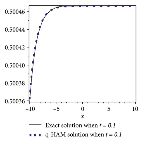
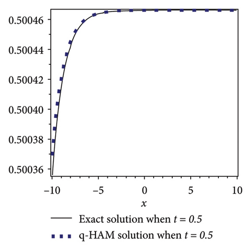
4.1.2. Graphical Comparison of q-HAM and Exact Solution for Example 1

In this subsection, comparison of q-HAM solution and exact solution for example 1 is presented graphically for fixed values of parameters at different time scales. Figures 1(a) and 1(b) show the accuracy and efficiency of the q-HAM.

4.1.3. The Convergence Analysis

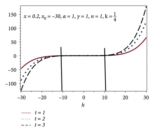
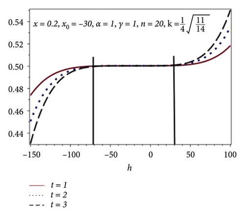
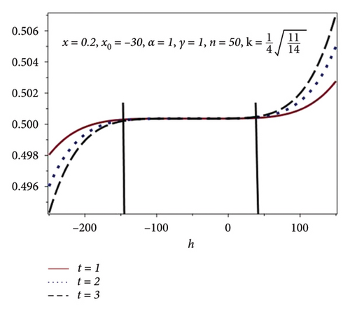
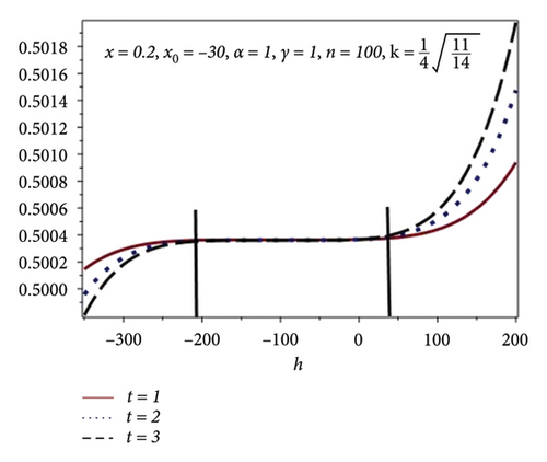
In this subsection, h-curves have been plotted for different values of n in Figures 2(a), 2(b), 2(c), and 2(d). Increasing behavior of convergence region is observed with the increasing values of n which is shown in Table 2. Figure 2 shows the h-curve of equation (15) for different values of the time scale against different values of n and fixed values x = 0.2, x₀ = −30, α = 1, γ = 1, and $$. Here, h is known as a convergence controlling parameter. From Figures 2(a), 2(b), 2(c), and 2(d), one can observe the increase in convergence region.

Table 2. Region of convergence for increasing values of n in the case of example 1.

n	h
1 (HAM)	−10 ≤ h ≤ 10
20	−70 ≤ h ≤ 30
50	−145 ≤ h ≤ 45
100	−210 ≤ h ≤ 48

4.2. Example 2

Here, we consider KSE taking periodic boundary conditions [29].

$$ ()

subject to IC,

$$ ()

The true solution of equation (24) is

$$ ()

Taking IC as an initial guess, we have

$$ ()

Using equation (27) in equation (18) and after integration, we get

$$ ()

Next, using equation (28) in equation (20) and after integration, we get

$$ ()

Likewise, one can evaluate the remaining terms of the series solution up to any required accuracy or a given tolerance.

4.2.1. The Error Analysis

In this subsection, comparison of the exact solution with the current results is presented. Table 3 uncovers the accuracy and applicability of q-HAM for solving highly nonlinear PDEs.

Table 3. Absolute error between approximate solution and exact solution when t = 0.0004.

x	Approximate solution (q-HAM)	Exact solution (25)	Absolute error
0	0.9999777363	0.9995999200	3.778 × 10−4
6.4	1.279733159	1.279615936	1.172 × 10−4
12.8	1.196518667	1.196791917	2.732 × 10−4
19.2	0.7001196027	0.7007569806	6.373 × 10−4
25.6	−0.05838957728	−0.05758743503	8.021 × 10−4
32	−0.01866102249	−0.01872761446	6.576 × 10−4

4.2.2. Graphical Comparison of Exact and q-HAM Solution for Example 2

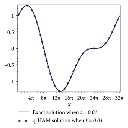
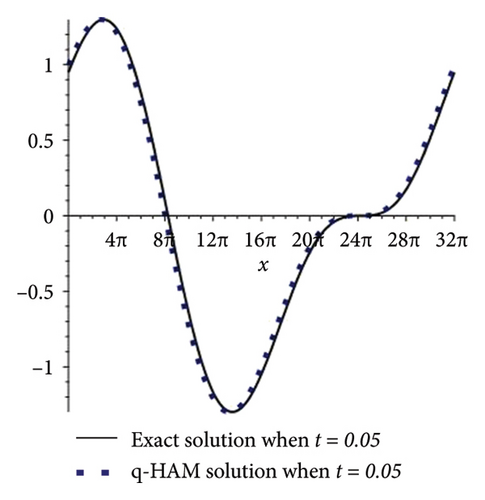
In this subsection, comparison of q-HAM solution and exact solution for example 2 are validated graphically for fixed values of parameters at different time scales. Figures 3(a) and 3(b) highlight the accuracy and applicability of q-HAM for periodic boundary conditions.

4.2.3. Convergence Analysis

In this section, form h-curves have been plotted for different values of n using Figures 4(a), 4(b), 4(c), and 4(d). Increase in the convergence region is observed with the increase of n as shown in Table 4. Figures 4(a), 4(b), 4(c), and 4(d) show the h-curve of equation (15) for different values of the time scale for different values of n and fixed values of x = 6.4, α = 1, γ = 1. From Figures 4(a), 4(b), 4(c), and 4(d), one can observe the increase in the convergence region for the increased values of n.

Table 4. Region of convergence for increasing values of “n” for example 2.

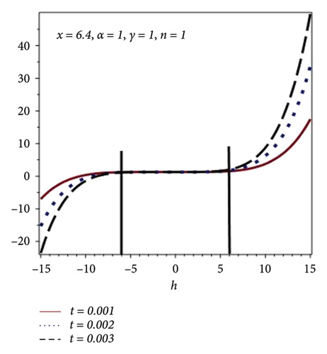
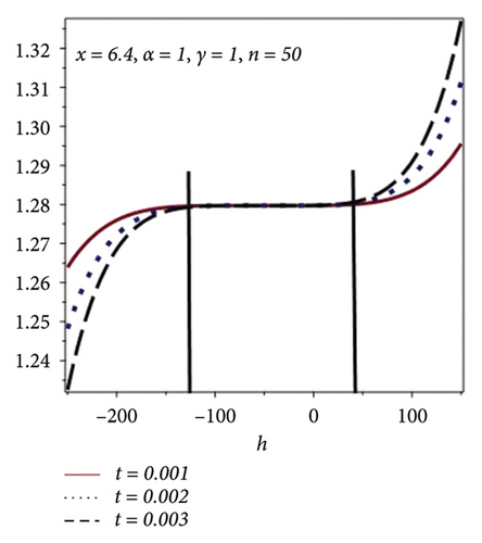
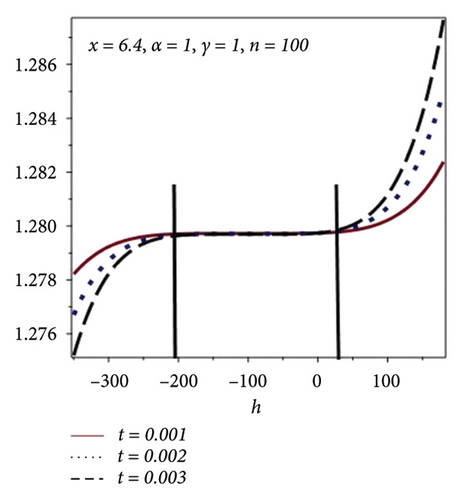
n	h
1 (HAM)	−6 ≤ h ≤ 6
20	−90 ≤ h ≤ 50
50	−150 ≤ h ≤ 48
100	−200 ≤ h ≤ 45

4.3. Example 3

Consider the KSE of the form for α = −1, γ = 1, β = 0 [30],

$$ ()

subject to initial condition (IC),

$$ ()

Using IC as an initial guess,

$$ ()

Using equation (32) in (18) and after integration, we get

$$ ()

Next, using equation (32) and (33) in equation (20), we get

$$ ()

Similarly, Ψ₃, Ψ₄, … can be calculated for n = 3,  4,  5, ….

4.3.1. The Error Analysis

The comparison analysis is carried out in this subsection for example 3 in Table 5. For this purpose, some fixed values of involved physical parameters are taken into consideration. Table 5 validates the applicability and effectiveness of q-HAM. The table is constructed for fixed parameter values $$.

Table 5. Comparison between exact and q-HAM solutions for different values of x and t.

x	t	Ψapproximate	Ψexact	Absolute error
−5	0.1	4.63803897006092	4.63803896999059	7.033 × 10−11
	0.5	4.63843960932536	4.63843955306175	5.626 × 10−8
	1	4.63980631834404	4.63981420314860	7.885 × 10−6
0	0.1	4.63779287238718	4.63779287237956	7.620 × 10−12
	0.5	4.63783494136028	4.63783493730662	4.054 × 10−9
	1	4.63798185888373	4.63798344165438	1.583 × 10−6
5	0.1	4.63776749758524	4.63776749758446	7.800 × 10−13
	0.5	4.63777179526045	4.63777179492130	3.392 × 10−10
	1	4.63778691685813	4.63778710621169	1.893 × 10−7

4.3.2. The Graphical Comparison

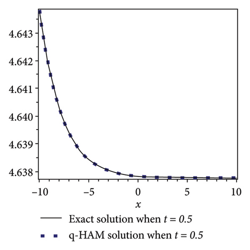
In this subsection, a comparison of q-HAM solution and exact solution for example 3 are presented graphically for some fixed values of involved factors at different time levels. Figures 5(a) and 5(b) highlight the accuracy and applicability of the q-HAM.

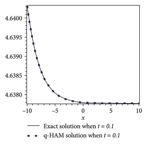
4.3.3. Convergence Analysis

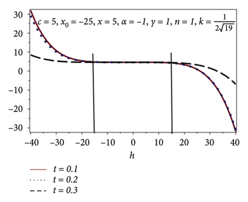
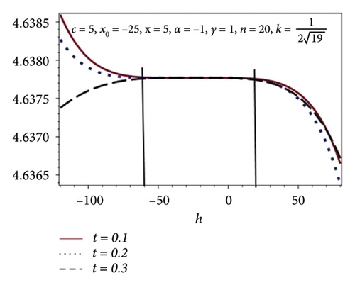
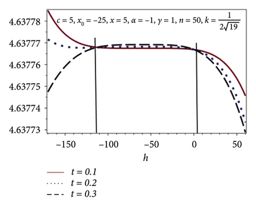
In this subsection, the h-curves are constructed through plots by taking some fixed values of the involved parameters in the model equation $$ and t = 0.1,  0.2,  0.3. The convergence region is calculated and is illustrated in Figure 6. It is observed that the convergence region upsurges as we increase the values of n. Similar behavior is also predicted in Table 6.

Table 6. Region of convergence for increasing values of “n” for example 3.

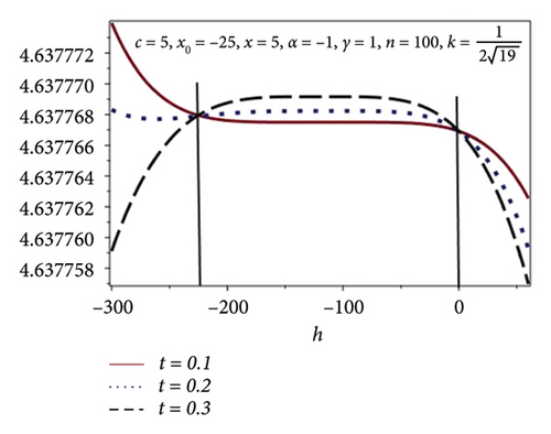
n	h
1 (HAM)	−15 ≤ h ≤ 15
20	−60 ≤ h ≤ 20
50	−115 ≤ h ≤ 5
100	−225 ≤ h ≤ 0

5. Conclusion

In this study, we find the approximate analytical solutions for various forms of KS equation using the q-HAM. The results are compared with the exact solution through absolute error tables which reveals a good agreement between computed solutions and the exact solutions. In Table 1, the q-HAM results are compared with the RDTM results for α = γ = 1, β = 0. The absolute error in Tables 1, 3, and 5 demonstrates that the q-HAM is more accurate than other methods like RDTM. The convergence analysis is performed using h-curves for each numerical example. The effectiveness and applicability of q-HAM are illustrated through h-curves in Figures 2(a), 2(b), 2(c), 2(d), 4(a), 4(b), 4(c), 4(d), 6(a), 6(b), 6(c), and 6(d). The convergence region for the embedded parameter h is calculated for some fixed values of independent variables x and t as well as other involved parameters. The accuracy of q-HAM is also explored through Figures 1(a), 1(b), 3(a), 3(b), 5(a), and 5(b) for examples 1, 2, and 3. A large convergence region is observed and tabulated in Tables 2, 4, and 6, highlighting the advantage of q-HAM over HAM. Given the fast convergence and ease of implementation of q-HAM, we plan to use this method for solving more complex and challenging problems in future.

Conflicts of Interest

The authors declare that they have no conflicts of interest.

Authors’ Contributions

Safdar Hussain contributed to the formal analysis, methodology, and writing the original draft. Abdullah Shah supervised the overall activities, editing and modifying the revised draft.