A Hybrid GARCH and Deep Learning Method for Volatility Prediction
Abstract
Volatility prediction plays a vital role in financial data. The time series movements of stock prices are commonly characterized as highly nonlinear and volatile. This study is aimed at enhancing the accuracy of return volatility forecasts for stock prices by investigating the prediction of their price volatility through the integration of diverse models. Thus, the study integrated four powerful methods: seasonal autoregressive (AR) integrated moving average (MA), generalized AR conditional heteroskedasticity (ARCH) family models, convolutional neural network (CNN), and bidirectional long short-term memory (LSTM) network. The hybrid model was developed using the residuals generated by the seasonal AR integrated MA model as input for the generalized ARCH model. Following this, the estimated volatility obtained was utilized as an input feature for both the hybrid CNNs and bidirectional LSTM models. The model’s forecasting performance was assessed using key evaluation metrics, including mean absolute error (MAE) and root mean squared error (RMSE). Compared to other hybrid models, our new proposed hybrid model demonstrates an average reduction in MAE and RMSE of 60.35% and 60.61%, respectively. The experimental results show that the model proposed in this study has good performance and accuracy in predicting the volatility of stock prices. These findings offer valuable insights for financial data analysis and risk management strategies.
1. Introduction
In financial terms, volatility denotes the degree of uncertainty or risk associated with fluctuations in the value of a security. Some securities exhibit high volatility, indicating significant fluctuations in their values over a wide range, while others demonstrate lower volatility, with their values varying within a narrower range. The fluctuations in securities’ returns are not directly observable, leading traders, institutional investors, and other market participants to understand the relationship between returns and volatility [1]. The global expansion of stock markets has sparked interest among researchers and practitioners in modeling the volatility of stock returns. Modeling volatility plays a crucial role in designing investment strategies to mitigate risk and enhance stock returns and in pricing securities and options [2]. Moreover, its significance extends beyond investors and market participants to encompass the broader economy. High levels of volatility can disrupt the stability of capital markets, affect currency values, and impede international trade [3]. In light of these consequential challenges, the necessity of forecasting volatility emerges as an imperative, ensuring investors can adeptly navigate the complexities of financial markets and make informed, stable investment decisions. Therefore, in this paper, the aim was to obtain an optimal model (a hybrid of GARCH and deep learning models) to predict volatility in stock prices.
The forecasting of volatility in financial instruments has been extensively examined in recent decades, primarily due to its role as an indicator that enables the estimation of risk associated with the asset within a specified time frame. In recent years, substantial literature has emerged on modeling and predicting volatility in financial markets. Primarily, Engle [4] developed the autoregressive (AR) conditional heteroskedasticity (ARCH) model by incorporating conditional variance and modeling the serial correlation of returns as a function of past errors and changing time. This was carried out as part of Engle’s attempts to explain how inflation dynamics operate in the United Kingdom.
To enhance Engle’s model, the GARCH models were developed by Bollerslev [5]. This enhancement involved incorporating a long memory and creating a more flexible lag structure by adding lagged conditional variance to the original model. The standard GARCH (SGARCH) model cannot model the leverage effect because its specifications assume that the variance depends on the shock’s magnitude and is independent of its sign [6].
Later, various adaptable GARCH models were introduced, incorporating additional parameters to capture the asymmetric behavior of time series data such as the exponential GARCH (EGARCH) model proposed by Nelson [7] and the threshold GARCH (TGARCH) model introduced by Zakoian [8].
B. Almansour, Alshater, and A. Almansour’s [9] research focused on assessing the effectiveness of ARCH and GARCH models in predicting volatility within the cryptocurrency market. The findings indicated that both positive and negative news events have a notable impact on conditional volatility across various cryptocurrency markets. Additionally, the study concluded that the GARCH model demonstrates promising predictive capabilities for cryptocurrency price movements in the market.
Franses and Van Dijk [10] conducted a study on forecasting stock market volatility using the nonlinear GARCH method. The investigation involved an analysis of the GARCH model and two of its nonlinear modifications to forecast weekly stock market volatility. The findings of the study indicated that the quadratic generalized ARCH (QGARCH) model was the most effective for forecasting the volatility of the stock market.
Sen, Mehtab, and Dutta [11] predicted the volatility of stocks from selected sectors of the National Stock Exchange (NSE) of the Indian economy using GARCH. The researchers found that asymmetric GARCH models, notably, provide more precise forecasts regarding the future volatility levels of the selected stocks. In a modified model, specifically concerning ARIMA-GARCH modeling as demonstrated by Aduda et al. [12], there has been an exploration of using the residuals of ARIMA as a vital factor for improving forecasting in GARCH.
Implementing deep learning models in financial markets, especially in stock markets, has become a burgeoning research subject in recent times due to the increasing use of artificial intelligence (AI) in various fields. Artificial neural network (ANN) models can capture the nonlinearity of the series, do not require the series to be stationary for modeling, and perform better in volatility forecasts than SGARCH-type models. Liu [13] showed that for a considerable time interval, volatility predictions for the Standard & Poor’s 500 (S&P 500) and Apple Inc. indicate that the long short-term memory (LSTM) can outperform the GARCH model.
In recent years, the field of financial time series analysis has witnessed a growing interest in the development of hybrid models that combine various deep-learning techniques with statistical models to enhance the accuracy of volatility prediction. Kim and Won [14] developed a hybrid model to predict the volatility of the Korea Composite Stock Price Index (KOSPI 200) by integrating GARCH-type models with the LSTM model.
Kakade et al. [15] investigated the advantage of hybridizing GARCH-type models with LSTM to predict the volatility of metals in the Indian commodity market. The study found that hybrid GARCH-LSTM models outperform standalone models. Vidal and Kristjanpoller [16] studied gold volatility prediction using a hybrid CNN-LSTM approach. This study found that the hybrid CNN-LSTM model outperforms the GARCH and LSTM models in forecasting the volatility of gold.
Zeng et al. [17] studied a natural gas load volatility prediction model by combining GARCH family models, the eXtreme Gradient Boosting (XGBoost) algorithm, and the LSTM network. Mademlis and Dritsakis [18] presented two hybrid models in the investigation of predictive models for the volatility of the Financial Times Stock Exchange Milano Italia Borsa (FTSE MIB) index and evaluated their efficacy alongside an asymmetric GARCH model and a neural network.
All the above studies have their limitations; for instance, hybrid SARIMA-GARCH family models for volatility forecasting often face limitations when confronted with nonlinear sequences and influential factors [19]. Moreover, a single Convolutional neural network (CNN) model has a poor interpretation of volatility. Therefore, prediction accuracy will not be high.
Combining hybrid econometric models such as SARIMA-GARCH family models with CNN models can effectively solve the shortcomings in volatility forecasting. CNN excels GARCH family models in capturing complex temporal patterns and nonlinear dependencies in volatility structures. Furthermore, CNN can automatically identify hierarchical features from the data, aiding in the extraction of meaningful representations and proving robust to noisy data.
However, integrating CNN with GARCH family models alone often fails to yield superior prediction results, as an abundance of feature inputs can degrade model performance. BiLSTM excels CNN in capturing long-term dependencies and sequential patterns in the data. By utilizing both forward and backward information patterns of the market, BiLSTM enhances accuracy in time series prediction. Its memory cells effectively handle data prone to irregular and seasonal patterns.
In response to this research gap, the present study introduces a novel hybrid SARIMA-GARCH-CNN-BiLSTM model. The forecasting performance of this new model is evaluated. The inclusion of BiLSTM in the extended model provides a significant improvement over the unidirectional approach of traditional LSTM models. The findings of this study provide valuable insights into understanding the movement and comovement of volatility prices, which is essential for investors, traders, and risk managers in navigating and mitigating the high-risk nature of these investments.
2. Methodology
The study used the SARIMA, GARCH family, CNN, and LSTM as components to create a new hybrid model. Each of these components has unique traits that may be extracted from historical data.
2.1. SARIMA Model
2.2. SGARCH Model
2.3. EGARCH Model
The EGARCH model achieves covariance stationarity when .
2.4. TGARCH Model
2.4.1. Model Selection Criteria
The study employed the most widely used model selection method, the Akaike information criterion (AIC) [23], to determine which GARCH model fits the data. The best possible model was selected based on the AIC scores of the models. AIC balances the goodness of fit against the complexity of the model. Lower AIC values indicate a better trade-off between fit and complexity.
2.5. CNN Model
This operation is called convolution.
CNNs are specialized neural networks designed for processing inputs with inherent spatial structures. Renowned for efficacy across diverse data formats such as one-dimensional time series data, two-dimensional image data, and three-dimensional video data [26], the study used the 1D-CNN model for sequential data. The network uses algorithms for data mining to automatically recognize and pick the most critical features from the raw data. The sequential 1D-CNN model was constructed using convolutional layers, pooling layers, and dense layers. The input was a 3D tensor with shape (batch size, time steps, and input dim).
The role of the convolutional layer in the CNN model is to identify temporal patterns and relationships within sequential data, such as time series [27]. The role of the pooling layer, on the other hand, is to perform downsampling to address computational complexity and achieve translation invariance, enabling the model to identify features regardless of location in the input. Furthermore, downsampling helps to minimize the likelihood of overfitting, increase computational efficiency, and decrease the number of parameters. CNNs combine concepts such as weight sharing and local connectivity to improve the model’s ability to do complex tasks. Relu is a popular activation function in CNNs due to its nonlinearity, computational efficiency, and ability to solve vanishing gradient problems of the training model in deep learning. While CNNs are effective models for time series forecasting applications, overfitting is a problem that can affect them. The overfitting problem can arise from factors such as the complexity of the model and highly correlated training data. Dropout is a regularization technique used in neural networks to prevent overfitting.
In this context l-th layer, denotes the i-th feature, refers to the j-th feature in the preceding (l − 1)-th layer, signifies the kernel connecting the i-th to the j-th features, is the bias associated with these features, and Relu stands for the activation function.
Figure 1 illustrates a diagram representing how feature maps are formed in a CNN model. In the diagram, u represents a sample filter with adjustable weights of Size 3. Each Ci denotes the i-th element of the feature map. N stands for the number of 1D data tensor units, and f represents the filter size with a stride of 1.

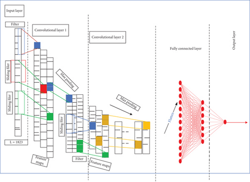
According to Rala Cordeiro et al. [29], the stride value defines how the kernel moves in the input data. The most common value is one, meaning that the kernel moves over one column of the input data at each iteration. After convolution, pooling reduces dimensionality and improves feature robustness. Pooling size corresponds to input feature units. It applies a function to multiple inputs (convolutional features). Max pooling defines the pooling layer. This study used two CNN layers to strike a balance between complexity and performance. This approach reduces the risk of overfitting by avoiding excessive complexity and mitigating challenges like vanishing or exploding gradients during training. Previous research, like [30], may support the efficacy of two-layer CNN architectures for the task at hand. The decision reflects a thoughtful consideration of computational efficiency and training stability. Figure 2 depicts the structure of a 1D-CNN model with two convolutional and two max pooling layers. The output of the last pooling layer is flattened and connected to a dense layer with N units. Following the final pooling layer, the output is flattened and connected to a dense layer containing N units. Subsequently, this dense layer is connected to the final output layer, which consists of a single neuron.
2.6. BiLSTM Model
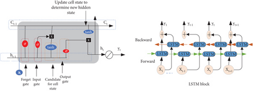
Hochreiter and Schmidhuber [31] first proposed the LSTM architecture as a specific type of recurrent neural network (RNN) to overcome the limitations of traditional RNNs in capturing and learning long-term dependencies in sequential data. While LSTM captures information from extended periods, the acquired data pertains to the time before the output moment, which lacks reverse information. However, for time series prediction, it is crucial to consider both backward and forward information patterns to enhance predictive performance. The two LSTMs that make up BiLSTM are forward and reverse. In contrast to the regular LSTM’s one-way state transfer, the BiLSTM takes into account the data’s changing laws both before and after data transmission, enabling it to make more thorough and precise decisions by utilizing both past and future knowledge. It has performed better than expected.
In Equation (9), denoted as ft, the forget gate mechanism. The sigmoid activation function σ was used to judge whether the last memory needs to be retained for the current memory state. Equation (7) describes the computation of it, serving as the input gate to assess the significance of retaining current input data. Equation (8) describes the calculation of , which is used to calculate the data that needs to be updated. Equation (10) shows whether the state at the current moment needs to be updated. After a new state was obtained, Equation (10) was used to calculate the output gate value Ot.
Figure 3 illustrates the internal organization of the BiLSTM model, constructed with LSTM blocks. BiLSTM, comprising both forward and backward LSTM components, necessitates a reversal of the computation.
2.7. SARIMA-GARCH-CNN-BiLSTM
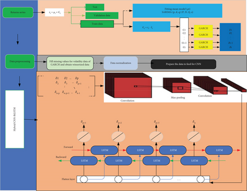
The study introduced a novel approach to volatility forecasting called the hybrid SARIMA-GARCH-CNN-BiLSTM Model. First, the mean model was built using SARIMA, which was well known for its ability to detect seasonal and temporal trends in financial time series data. Second, the volatility was estimated using three models from the GARCH family: GARCH, TGARCH, and EGARCH. This makes it easier to choose the most accurate model among the GARCH variations. As a result, asymmetry and time-varying patterns can be captured. SARIMA residuals were used as input to estimate volatility in the GARCH family models. Lastly, CNN and BiLSTM architectures receive the predicted output of the GARCH family models. CNN effectively captures spatial dependencies, while BiLSTM excels at capturing long-term dependencies, leveraging both temporal and spatial features for improved forecasting.
2.7.1. Model Development Procedure
The overall process of modeling followed the following algorithms.
2.7.2. Data Preprocessing
- 1.
Filling missing data. Due to the closure of financial markets on weekends (Saturdays and Sundays) and public holidays, missing values may occur in stock datasets. Additionally, issues with processing and registration during the data retrieval process could contribute to missing data. Incomplete data introduces biases due to discrepancies between observed and unobserved data. In time series prediction, it is essential to address this issue without discarding values from the series [32]. In this study, cubic spline interpolation was used to capture complex and nonlinear trend structures that linear methods cannot adequately handle. In cubic spline interpolation, the cubic spline polynomial is fit to time series data to estimate the missing values.
- 2.
Outlier detection. Data points that are located at the outermost limits of a dataset are referred to be outliers.
- 3.
Data normalization. The winsorized data, devoid of outliers, originates from various forecasting points, each exhibiting different scales of values. To address this issue and enhance the training efficiency of the model, min–max normalization, as represented in Equation (15), is employed to scale the dataset within the range of (0, 1].
- 4.
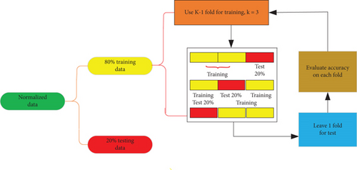
Data splitting. To create and assess a forecasting model, the normalized data needs to be divided. In practice, there has not been a universally perfect percentage for data splitting in the past. Nonetheless, there are various methods to partition the dataset. One instance involves an 80% training and 20% testing split [24, 34], while another approach entails allocating 70% to the training dataset, 15% to the validation dataset, and 15% to the test dataset [35]. Figure 4 presents the data splitting procedure utilized in this research, illustrating the allocation of datasets. In this study, the data is divided into three segments (60:20:20 ratio), facilitating a thorough model assessment. The training set educates the model about underlying patterns, while the validation set serves as an impartial benchmark for comparing algorithms trained on this data. Subsequently, the test set evaluates the model’s performance on fresh data, ensuring a robust evaluation process and guarding against overfitting. Furthermore, to bolster model training and minimize overfitting, a k = 3-fold cross-validation technique is utilized within the training dataset.
After splitting the data, it has to be reshaped into 3D to be an input for the hybrid CNN-BiLSTM model. Thus, input dimensions are samples, time steps, and features. The number of time steps (window size) was a hyperparameter that represents the number of previous lags used as input to predict the next time steps. The study used empirical testing to fix an optimal value of the window hyperparameter. The sequence of observations {x1, x2, ⋯, xn} have to be changed to multiple examples (samples) by developing a matrix X which served as the independent variable of the model and y as the dependent variable of the model of which the model can learn. Then, divide the time series to n − p + 1 examples where each sample has a size equal to the number of time steps (lagged variables) that is p and the size of learning samples is n + 1. The obtained size of the independent and predicted matrix will have a size (n − p + 1) × p and (n + 1) × 1. The deep learning models described in this paper are outlined in Table 1. The goal is to pick out features from the input dataset using CNN layers. After that, the outputs of these CNN layers are passed into BiLSTM layers and a dense layer at the output to help predict sequences. The comprehensive architecture of the hybrid SARIMA-GARCH-CNN-BiLSTM model is detailed in Figure 5. This structure begins by leveraging the return series of Apple Inc.’s price data to establish the mean model. Subsequently, it analyzes the residuals of the mean model to estimate volatility using GARCH models. Finally, it preprocesses the GARCH model outputs to serve as inputs for the hybrid CNN-BiLSTM model.
| HDL model | Structure of layer |
|---|---|
| CNN | conv1D layer (filters: 256, filter size: 2, Relu activation) + maxpooling1D (pooling size: 2, padding: same) + conv1D layer (filters: 128, filter size: 2, Relu activation) + maxpooling1D (polling size: 2, padding: same) + flatten layer + dense layer (neuron: 1, Relu activation) + dropout =0.2 with fully connected layer (neurons =1: linear activation) |
| CNN-BiLSTM | conv1D layer (filters: 256, filter size: 2, Relu activation) + maxpooling1D (pooling size: 2, padding: same) + conv1D layer (filters: 128, filter size: 2, Relu activation) + maxpooling1D (polling size: 2, padding: same) + flatten layer + BiLSTM layer (neurons: 128, Relu activation) + BiLSTM layer (neurons: 50, Relu activation) + dense layer (neuron: 1, linear activation) |
2.8. Forecasting Performance Evaluation
3. Data
4. Result and Discussion
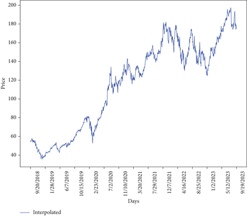
The Apple Inc. price series in Figure 6 illustrates long-term increasing and decreasing trends. It suggests a nonstationarity series. Since the price series exhibits nonstationarity, the study applies a logarithmic transformation and takes the first difference at lag 1 to obtain the return series. Thus, when examining higher kurtosis in original return data, as shown in Table 2, it is desirable to winsorize data to make it less susceptible to outliers. Figure 7 displays the distribution of returns and winsorized returns through box plots, showcasing their respective central tendencies and dispersion. Due to the detection of outliers in the return data, the study opted to winsorize the dataset as shown in Figure 7. Table 2 shows the summary statistics of the returns and winsorized returns. The Jarque–Bera test rejects the normality assumption for both returns. With negative kurtosis, a lighter tail, and fewer outliers in the winsorized returns, the study utilized the depicted winsorized returns data in Table 2 for further analysis.
| Statistic | Original returns | Winsorized returns |
|---|---|---|
| Mean | 0.000648 | 0.000715 |
| Median | 0.000617 | 0.000617 |
| Variance | 0.000299 | 0.00017 |
| Skewness | −0.128 | −0.084 |
| Kurtosis | 5.52139 | −0.3254 |
| Jarque–Bera | 2316.86 | 10.2145 |
| p value | 0.00 | 0.006 |
| Sample size | 1820 | 1820 |
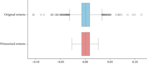
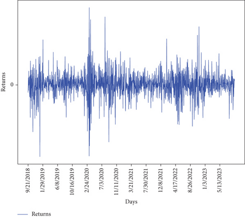
Figure 8 displays the winsorized graph that fluctuated above and below the 0 lines, indicating that the price series achieved stationarity in the mean. However, the series is not stationary in variance.
The study also tested for stationarity using the augmented Dickey–Fuller test. The ADF test result displayed in Table 3 rejects the null hypothesis of a unit root’s existence, supported by the ADF test value of −10.2166 and a p value of 0.02576. It is safe to say that the winsorized daily returns are stationary.
| Daily Apple Inc. winsorized returns (rt) | |||
|---|---|---|---|
| Test | Statistic | Critical values | pvalue |
| ADF | −10.2166 | % critical value: −3.4339 | 0.025 |
| % critical value: −2.8631 | |||
| % critical value: −2.5676 | |||
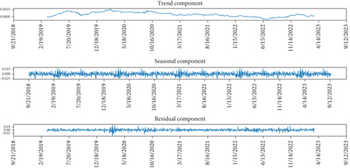
The visual representation of the decomposition of the return time series is shown in Figure 9. This decomposition separates the series into three distinct components: trend, seasonal, and residuals. It is evident from the figure that the observed series exhibits seasonality with a period of two.
The study employed the AIC for choosing the order, as it effectively minimizes prediction error and is asymptotically comparable to cross-validation [39]. Table 4 summarizes the AIC values of different models. After assessing various SARIMA models, the most suitable model for the observed series was ARIMA(0, 0, 1)(1, 0, 0)2, which exhibits the lowest AIC value of −5993.920.
| Model | AIC |
|---|---|
| ARIMA(1,0,0)(1,0,0)2 | −5993.333 |
| ARIMA(0,0,1)(0,0,1)2 | −5993.063 |
| ARIMA(1,0,0)(1,0,1)2 | −5992.025 |
| ARIMA(1,0,0)(0,0,1)2 | −5992.182 |
| ARIMA(1,0,1)(1,0,0)2 | −5992.183 |
| ARIMA(0,0,1)(1,0,0)2 | −5993.920 |
| ARIMA(0,0,1)(1,0,1)2 | −5992.0 |
| Coef. | Std. err. | z | P > |z| | 0.025 | 0.975 | |
|---|---|---|---|---|---|---|
| Intercept | 0.0011 | 0.001 | 1.660 | 0.097 | 0.001 | 0.002 |
| ma.L1 | 0.1998 | 0.017 | 12.014 | 0.001 | 0.167 | 0.232 |
| ar.S.L2 | −0.2096 | 0.018 | −11.902 | 0.001 | −0.244 | −0.1375 |
| Sigma2 | 0.0003 | 0.00659 | 46.658 | 0.001 | 0.000 | 0.000 |
At a significance level of 5%, Engle’s Lagrange Multiplier ARCH test, employing up to 21 lags representing a 1-month trading period of Apple Inc., as presented in Table 6, rejects the null hypothesis of no ARCH effects in the winsorized returns. This means that the variances of returns were heteroscedastic and suggested the use of the ARCH/GARCH model for capturing the time-varying volatility in the returns. Furthermore, the result was supported by the Ljung–Box test, which indicated that the residuals were uncorrelated and that the squared residuals did not exhibit serial correlation. In simpler terms, the error variance exhibited autocorrelation. Next, a distribution for the residuals of the return series was estimated to approximate the empirical distribution. Based on the work conducted by Budiarti et al. [40], the study examined the distribution of residuals. A comparison was made among the standard residuals of three distributions, namely, normal distribution, t-student distribution, and logistic distribution, against the empirical distributions, as depicted in Figure 10.
| Lag | Statistics | pvalue | |
|---|---|---|---|
| For residual series | |||
| ARCH-LM | Lag 1 | 99.0427 | 0.001 |
| Lag 21 | 153.3352 | 0.001 | |
| Ljung–Box | Lag 1 | 0.008505 | 0.926522 |
| Lag 21 | 8.949068 | 0.111113 | |
| For squared residual series | |||
| Ljung–Box | Lag 1 | 100.864047 | 265.57485 |
| Lag 21 | 0.0096 | 0.00249 | |
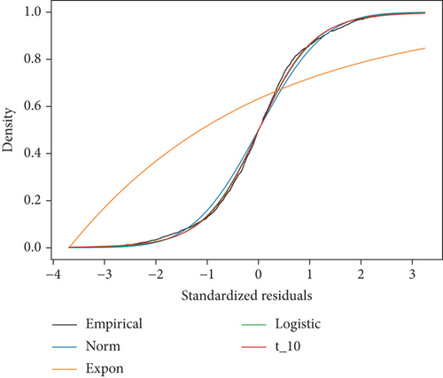
The Anderson–Darling test showed that the most suitable distribution for Apple Inc. residual data was the logistic distribution, as shown in Table 7.
| pvalue | Best fit | ||
|---|---|---|---|
| Expo | ∞ | 1.34 | 0 |
| Norm | 20.167945 | 0.784 | 0 |
| Logistic | 4.936475 | 0.66 | 1 |
| t-student | 90.8091 | 1.24 | 0 |
The study applied three variants of GARCH family models: SGARCH, EGARCH, and TGARCH, to the residuals of SARIMA for model identification. The AIC and log-likelihood of the estimated models are noted for each of the models.
4.1. SARIMA-SGARCH Model Identification
The SARIMA(0,0,1)(0,0,1)2-SGARCH(1,2) model under the logistic distribution was favored over the other models due to its smallest AIC value (979.6836) and larger log-likelihood (−485.842), as indicated in Table 8.
| Model | AIC | Log-likelihood |
|---|---|---|
| SARIMA(0,0,1)(1,1,0)2-SGARCH(1,1) | 1008.52 | −501.259 |
| SARIMA(0,0,1)(1,1,0)2-SGARCH(1,2) | 979.6836 | −485.842 |
| SARIMA(0,0,1)(0,1,1)2-SGARCH(2,1) | 1010.5175 | −501.255 |
| SARIMA(0,0,1)(1,1,1)2-SGARCH(2,2) | 981.6836 | −485.842 |
4.2. SARIMA-TGARCH Model Identification
The SARIMA(0,0,1)(0,0,1)2-TGARCH(1,2,1) model under the logistic distribution was favored over the other models due to its smallest AIC value (981.476) and larger log-likelihood (−485.476), as illustrated in Table 9.
| Model | AIC | Log-likelihood |
|---|---|---|
| SARIMA(0,0,1)(1,1,0)2-TGARCH(1,1,1) | 1010.28 | −501.139 |
| SARIMA(0,0,1)(1,1,0)2-TGARCH(1,1,2) | 1012.28 | −501.139 |
| SARIMA(0,0,1)(0,1,1)2-TGARCH(1,2,1) | 981.476 | −485.476 |
| SARIMA(0,0,1)(1,1,1)2-TGARCH(2,1,1) | 1012.28 | −501.139 |
| SARIMA(0,0,1)(1,1,1)2-TGARCH(1,2,2) | 983.476 | −485.738 |
| SARIMA(0,0,1)(1,1,1)2-TGARCH(2,1,2) | 1014.28 | −501.139 |
| SARIMA(0,0,1)(1,1,1)2-TGARCH(2,2,1) | 983.476 | −485.738 |
| SARIMA(0,0,1)(1,1,1)2-TGARCH(2,2,2) | 985.476 | −485.738 |
4.3. SARIMA-EGARCH Model Identification
The SARIMA(0,0,1)(0,0,1)2-EGARCH(1,1,2) model under the logistic distribution was favored over the other models due to its smallest AIC value (−730.704) and larger log-likelihood (372.352), as demonstrated in Table 10.
| Model | AIC | Log-likelihood |
|---|---|---|
| SARIMA(0,0,1)(1,1,0)2-EGARCH(1,1,1) | −617.779 | −584.740 |
| SARIMA(0,0,1)(1,1,0)2-EGARCH(1,1,2) | −730.704 | 372.352 |
| SARIMA(0,0,1)(0,1,1)2-EGARCH(1,2,1) | −671.070 | 342.535 |
| SARIMA(0,0,1)(1,1,1)2-EGARCH(2,1,1) | −730.284 | 691.738 |
| SARIMA(0,0,1)(1,1,1)2-EGARCH(1,2,2) | −730.594 | 686.541 |
| SARIMA(0,0,1)(1,1,1)2-EGARCH(2,1,2) | −728.706 | −684.653 |
| SARIMA(0,0,1)(1,1,1)2-EGARCH(2,2,1) | −687.262 | 351.631 |
| SARIMA(0,0,1)(1,1,1)2-EGARCH(2,2,2) | −728.601 | 371.301 |
| Models | Model parameters | Coefficients | pvalues |
|---|---|---|---|
| SGARCH(1,2) | Intercept (ω) | 0.0177 | 0.07805 |
| α1 | 0.2337 | 0.02582 | |
| β1 | 0.3201 | 0.07668 | |
| β2 | 0.4431 | 0.01286 | |
| TGARCH(1,2,1) | Intercept (ω) | 0.0177 | 0.07.602 |
| α1 | 0.2338 | 0.02499 | |
| β1 | 0.2147 | 0.047391 | |
| β2 | 0.4223 | 0.01255 | |
| γ1 | −0.2338 | 0.939 | |
| EGARCH(1,1,2) | Intercept (ω) | 1.9742 | 0.01346 |
| α1 | 2.5914 | 0.06552 | |
| β1 | 0.9946 | 0.001 | |
| γ1 | −0.7159 | 0.619 | |
| γ2 | −1.5419 | 0.02563 | |
Equation (20) shows the mean and volatility model of hybrid SARIMA(0,0,1)(1,0,0,2)-SGARCH(1,2). In the hybrid SARIMA(0,0,1)(1,0,0,2)-SGARCH(1,2) model, the degree of volatility persistence was found to be 0.9969. Given that the persistence parameter was very close to unity, volatility was predictable for future periods.
From Equation (22), γ1 = −0.2338 ≠ 0 indicates that there exists a leverage effect. In addition to this, γ1 < 0 indicates that volatility increased more by positive shocks than negative shocks at equal length.
4.4. The Prediction Results of Hybrid Econometric Models
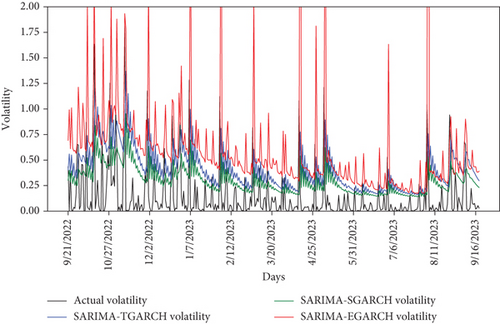
As shown in Figure 11, it is the fitting curve of the predicted value and the true value of every hybrid econometric model. It can be seen that the fitting effect of the hybrid SARIMA-SGARCH model was better than the other two models. As shown in Table 12, it is the value of the evaluation index of hybrid econometric models. Thereinto, the value of MAE (0.2053) and RMSE (0.2731) of hybrid SARIMA-SGARCH is the smallest. Therefore, the overall performance of the hybrid SARIMA-SGARCH model is better. However, these hybrid econometric models did not show good prediction performance because they did not capture complex nonlinear relationships and sequential dependencies of the data.
| Model | MAE | RMSE |
|---|---|---|
| Hybrid SARIMA-SGARCH | 0.2053 | 0.2731 |
| Hybrid SARIMA-EGARCH | 0.444 | 1.1706 |
| Hybrid SARIMA-TGARCH | 0.2601 | 0.3281 |
4.5. Prediction Results of Hybrid Econometric Models With CNN Model
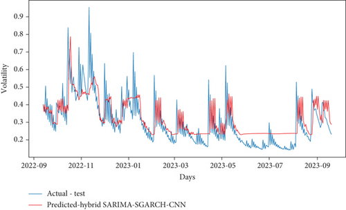
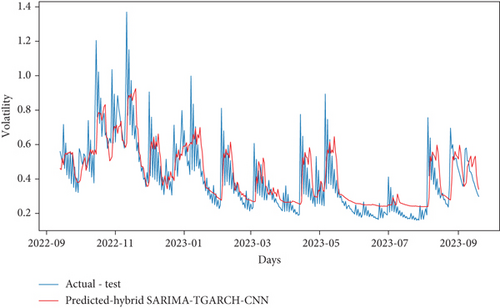
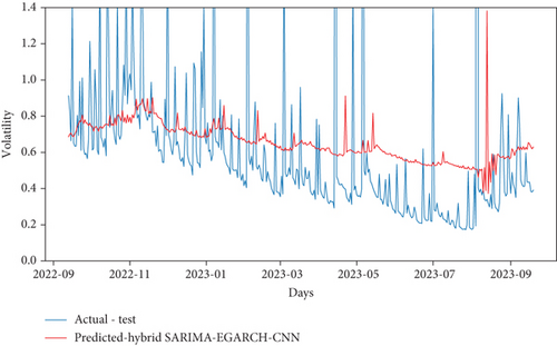
Through the above prediction, it is found that the hybrid SARIMA-SGARCH model has a better fitting effect and higher prediction accuracy than the prediction results of the other two econometric models. Furthermore, to improve the prediction accuracy of volatility, rely on (1) hybrid econometric models to describe the series pattern and volatility clustering and (2) the CNN model to capture spatial patterns and local dependencies in the data, enhancing model robustness and accuracy. Through this experiment, the study used the estimated volatilities of hybrid econometric models as input features for the CNN model. The prediction results of hybrid econometrics with CNN models are shown in Figures 12(a), 12(b), and 12(c), while the corresponding evaluation outcomes are summarized in Table 13. Through the prediction results and evaluation results, it can be found that, compared with hybrid SARIMA-SGARCH, the MAE and RMSE of hybrid SARIMA-SGARCH-CNN decreased by 65% and 66.7%, respectively. The MAE and RMSE of the hybrid SARIMA-EGARCH-CNN increased by 36.3% and 75.4%, respectively. The MAE and RMSE of the hybrid SARIMA-TGARCH-CNN decreased by 51.5% and 54.5%, respectively. The MAE and RMSE values for hybrid SARIMA-SGARCH-CNN are the lowest among the models considered, indicating its superior overall performance. However, despite these favorable metrics, the hybrid SARIMA-SGARCH-CNN model exhibited suboptimal prediction performance. This limitation could stem from its inability to effectively capture sequential patterns and long-term dependencies within the data.
| Model | MAE | RMSE |
|---|---|---|
| Hybrid SARIMA-SGARCH-CNN | 0.0717 | 0.0909 |
| Hybrid SARIMA-EGARCH-CNN | 0.3223 | 1.1120 |
| Hybrid SARIMA-TGARCH-CNN | 0.099510 | 0.12419 |
4.6. Prediction Results of the Proposed Hybrid Econometrics With Hybrid CNN-BiLSTM Model
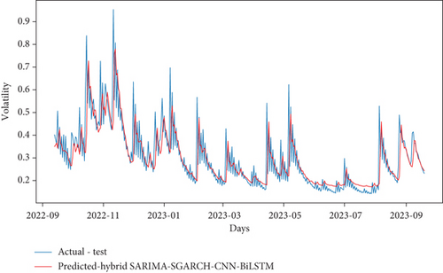
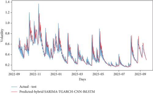
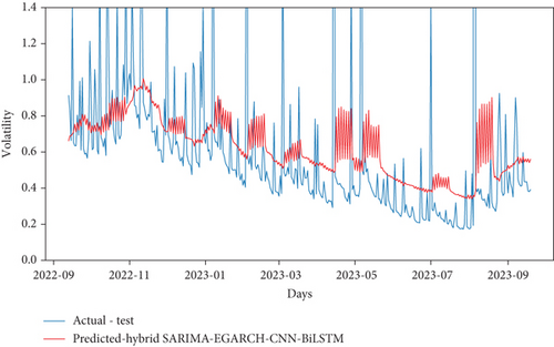
The study introduced three novel hybrid models, denoted as hybrid SARIMA-SGARCH-CNN-BiLSTM, hybrid SARIMA-EGARCH-CNN-BiLSTM, and hybrid SARIMA-TGARCH-CNN-BiLSTM, and conducted comparative analyses with existing hybrid econometric models and hybrid econometric models incorporating CNN. Additionally, the study performed intercomparisons among the newly proposed hybrid models to identify the superior-performing model. Now, the new models are constructed by taking the forecasted volatility of hybrid econometric models as input features to the hybrid CNN-BiLSTM model to capture dependencies from both past and future contexts. The prediction results of the newly proposed models are shown in Figures 13(a), 13(b), and 13(c). The evaluation results of the model are presented in Table 14. In comparison to hybrid SARIMA-SGARCH-CNN, the hybrid model hybrid SARIMA-SGARCH-CNN-BiLSTM exhibited notable improvements, with a decrease of 28.3% in MAE and 22.3% in RMSE. Conversely, hybrid SARIMA-EGARCH-CNN-BiLSTM experienced an increase of 74.7% in MAE and 91.8% in RMSE compared to hybrid SARIMA-SGARCH-CNN. Similarly, hybrid SARIMA-TGARCH-CNN-BiLSTM showed a slight increase of 1.7% in MAE and 23.3% in RMSE relative to hybrid SARIMA-SGARCH-CNN. Moreover, hybrid SARIMA-SGARCH-CNN-BiLSTM demonstrated superior performance compared to hybrid SARIMA-EGARCH-CNN-BiLSTM, with a significant decrease of 81.9% in MAE and 93.6% in RMSE. Additionally, hybrid SARIMA-SGARCH-CNN-BiLSTM outperformed hybrid SARIMA-TGARCH-CNN-BiLSTM, with reductions of 29.5% in MAE and 40.5% in RMSE. Similarly, hybrid SARIMA-TGARCH-CNN-BiLSTM exhibited improvements over hybrid SARIMA-EGARCH-CNN-BiLSTM, with reductions of 58.2% in MAE and 89.3% in RMSE. Notably, among the newly proposed hybrid models, hybrid SARIMA-SGARCH-CNN-BiLSTM demonstrated superior predictive accuracy compared to all hybrid econometric models with CNN-BiLSTM, indicating its efficacy in forecasting. Consequently, the hybrid SARIMA-SGARCH-CNN-BiLSTM model stands out as the most effective in achieving optimal prediction performance and the highest accuracy among the proposed models.
| Model | MAE | RMSE |
|---|---|---|
| Hybrid SARIMA-SGARCH-CNN-BiLSTM | 0.0514 | 0.0706 |
| Hybrid SARIMA-EGARCH-CNN-BiLSTM | 0.2840 | 1.1110 |
| Hybrid SARIMA-TGARCH-CNN-BiLSTM | 0.07301 | 0.11864 |
Based on the obtained results, the hybrid SARIMA-SGARCH-CNN-BiLSTM model outperformed other hybrid econometric models, showing an average reduction in MAE and RMSE of 81.9% and 82.25%, respectively. Additionally, the hybrid SARIMA-SGARCH-CNN-BiLSTM model exhibited superior performance compared to hybrid econometrics with CNN models, with an average reduction in MAE and RMSE of 53.5% and 52.8%, respectively. Moreover, compared to hybrid SARIMA-GARCH family models, the outperformed hybrid of econometrics with CNN-BiLSTM demonstrates an average reduction in MAE and RMSE of 55.5% and 67%, respectively. The outcomes indicate that the hybrid SARIMA-SGARCH-CNN-BiLSTM model outperformed its counterparts, the hybrid econometrics with CNN-BiLSTM models, exhibiting notable improvements. This model showcased an average reduction in MAE and RMSE of 55.5% and 67%, respectively, underscoring its enhanced predictive accuracy and efficiency. Compared to three distinct hybrid models, the proposed hybrid SARIMA-STANDARD-GARCH-CNN-BiLSTM model demonstrates an average reduction in MAE and RMSE of 60.35% and 60.6%, respectively. Overall, the hybrid SARIMA-SGARCH-CNN-BiLSTM model emerged as the top performer among the various hybrid econometric models evaluated in this study. These findings underscore the effectiveness of the SARIMA-SGARCH-CNN-BiLSTM approach in volatility forecasting.
5. Conclusion
Based on the findings presented in the study, the following conclusions were drawn. The study used the input as residuals of the SARIMA model for three hybrid econometric models and selected the best model. The results showed that the hybrid SARIMA-SGARCH model outperformed the other two hybrid models. Additionally, the study incorporated the estimated volatilities of the econometric models as input features to the CNN to enhance prediction accuracy. The results indicated that the hybrid SARIMA-SGARCH-CNN model outperformed the hybrid SARIMA-EGARCH-CNN and hybrid SARIMA-TGARCH-CNN models. Finally, the study constructed three new models and used the estimated volatility of the hybrid econometrics as input to the CNN-BiLSTM model, concluding that the hybrid SARIMA-SGARCH-CNN-BiLSTM model performs well. This proposed model demonstrated its effectiveness, particularly with Apple Inc. data, providing valuable insights for financial data analysis and risk management strategies, thus aiding investors in making informed decisions.
6. Recommendation
The study was limited to investigating the volatility prediction of Apple Inc. using the three new hybrids of econometrics with CNN-BiLSTM models. As a result, the following aspects for further investigation are suggested. Future studies should explore incorporating attention mechanisms or transformer architectures to capture complex temporal dependencies and improve forecasting accuracy. Additionally, evaluating the impact of incorporating additional data sources beyond historical stock prices, such as sentiment analysis and financial news, could augment the forecast model. Furthermore, extending the research to include volatility forecasting for a portfolio of assets and exploring correlations between the assets is recommended.
Conflicts of Interest
The authors declare no conflicts of interest.
Funding
This work is supported by the Pan African University Institute for Basic Sciences, Technology and Innovation.
Acknowledgments
This work is supported by the Pan African University Institute for Basic Sciences, Technology and Innovation.
Open Research
Data Availability Statement
The data of this study can be obtained by contacting the corresponding author.


