International Journal of Energy Research

Volume 2024, Issue 1 5630435

Research Article

Open Access

Combination of Physics-Based Model and Artificial Intelligence for Rapid Simulation and Optimization of Dark Fermentative Hydrogen Production From Water Hyacinth

Phan Khanh Thinh Nguyen

orcid.org/0000-0002-8204-6701

Department of Chemical and Biological Engineering , Gachon University , Seongnam , 13120 , Gyeonggi-do , Republic of Korea , gachon.ac.kr

Search for more papers by this author

Thi Thu Ha Tran,

Corresponding Author

Thi Thu Ha Tran

[email protected]

orcid.org/0000-0001-7191-8714

Faculty of Environment , Ho Chi Minh City University of Natural Resources and Environment , Tan Binh District, Ho Chi Minh City , Vietnam , hcmunre.edu.vn

Search for more papers by this author

Tuan Loi Nguyen,

Corresponding Author

Tuan Loi Nguyen

[email protected]

orcid.org/0000-0002-5622-4359

Institute of Fundamental and Applied Sciences , Duy Tan University , Ho Chi Minh City , 70000 , Vietnam , duytan.edu.vn

Faculty of Environmental and Chemical Engineering , Duy Tan University , Da Nang City , 50000 , Vietnam , duytan.edu.vn

Search for more papers by this author

Phan Khanh Thinh Nguyen,

Phan Khanh Thinh Nguyen

orcid.org/0000-0002-8204-6701

Department of Chemical and Biological Engineering , Gachon University , Seongnam , 13120 , Gyeonggi-do , Republic of Korea , gachon.ac.kr

Search for more papers by this author

Thi Thu Ha Tran,

Corresponding Author

Thi Thu Ha Tran

[email protected]

orcid.org/0000-0001-7191-8714

Faculty of Environment , Ho Chi Minh City University of Natural Resources and Environment , Tan Binh District, Ho Chi Minh City , Vietnam , hcmunre.edu.vn

Search for more papers by this author

Tuan Loi Nguyen,

Corresponding Author

Tuan Loi Nguyen

[email protected]

orcid.org/0000-0002-5622-4359

Institute of Fundamental and Applied Sciences , Duy Tan University , Ho Chi Minh City , 70000 , Vietnam , duytan.edu.vn

Faculty of Environmental and Chemical Engineering , Duy Tan University , Da Nang City , 50000 , Vietnam , duytan.edu.vn

Search for more papers by this author

First published: 26 October 2024

https://doi.org/10.1155/2024/5630435

Citations: 3

Academic Editor: Prakash Bhuyar

Share a link

Email
Wechat
Bluesky

Abstract

Dark fermentative hydrogen (H₂) production from water hyacinth (WH) is considered a potentially sustainable process that helps minimize this weed’s harmful effects on the ecosystem and dependence on fossil fuels. To create a quick and precise tool for simulating and optimizing this process, this study applied the combination of the physics-based model and artificial intelligence approaches for the first time. The physics-based model was used as a computational experimental dataset generator to save time and cost in acquiring experimental data. Such a synthetic dataset was used to train the artificial neural network (ANN) model, which can predict the performance of dark fermentation fed with water hyacinth (DF@WH) in a fraction of the time. The particle swarm optimization (PSO) algorithm was then integrated to identify the ideal conditions for DF@WH. H₂ productivity and total energy recovery were selected as objectives based on basic operating parameters such as substrate concentration, initial pH, temperature, and operating time. The optimization results revealed that the maximum values of H₂ productivity (i.e., the maximum yield of 266.8 mL/g-TS and the maximum rate of 80.5 mL/L/h) and energy efficiency (i.e., 11.4%) cannot be achieved simultaneously under a specific optimal condition. Instead, when these targets were considered equally important, the balance optimal condition was determined at a substrate concentration of 8.9 g-TS/L, an initial pH of 6.5, a temperature of 33.9°C, and an operating time of 28.2 h. Under such conditions, H₂ productivity can be achieved with a yield of 200.2 mL/g-TS at a production rate of 62.9 mL/L/h and a total energy recovery of 11.0%.

1. Introduction

Due to its nontoxic nature, carbon-free properties, and high energy density, hydrogen (H₂) is considered a green fuel for sustainable energy solutions [1]. However, to date, H₂ has been primarily produced through thermal cracking or steam reforming of fossil carbon–based sources, despite their practicality, significantly contributing to emissions and reducing H₂ sustainability [2, 3]. From that situation, H₂ production from green and clean sources through biological processes has received increasing research attention [4]. Among them, dark fermentative hydrogen (H₂) production from water hyacinth (WH) is considered a potentially sustainable process that helps minimize this weed’s harmful effects on the ecosystem and dependence on fossil fuels. As known, WH is a noxious weed that damages agricultural and aquatic ecosystems [5]. Its vigorous growth depletes oxygen and nutrient content, leading to plant and animal death. Meanwhile, dark fermentation (DF) is gaining interest due to its low investment and operating costs and environmental friendliness [6]. Even so, DF fed with water hyacinth (DF@WH) is a complex process, and its performance is affected by various parameters, such as substrate concentration, initial pH, temperature, and inoculum type [7–15]. Many experimental studies on DF@WH have been carried out [7–15]; however, optimization studies for this process are currently absent in the literature. In general, the optimization for DF can be implemented via response surface methodology (RSM) [16, 17]. However, the exclusive use of quadratic polynomial models has resulted in RSM often being ineffective for complicated processes [18, 19]. Moreover, with the large number of independent variables to be investigated, the necessary expenses and time for the experiments involved will significantly increase [20].

In that context, mathematical model-based optimization has been regarded as a valuable tactic for cutting down on experimental expenses and time [21]. The mathematical models for DF can be divided into physics-based models and data-driven models. The physics-based models, also known as equation-based models, are developed based on the fundamental physical principles that enable them to comprehensively describe the behavior of processes [22–24]. However, such physics-based models are too complex, requiring high computational effort and time-consuming, thus preventing their application in control or online applications. Moreover, requiring the simultaneous solution of nonlinear equations with many variables, it is challenging to apply optimization algorithms to these physics-based models [22–24].

Conversely, data-driven models have been considered practical mathematical tools in online applications and control due to they can be simulated and optimized with quick computational turnaround times [23, 25]. One of the common examples of a data-driven model is the artificial neural network (ANN), which mimics the functioning of the human brain and is capable of creating complex relationships between predictors and responses without the need for explicit physical formulations [25]. Compared to RSM, ANN has been proven to be superior in terms of predictive ability and convenience [18, 19, 25]. Most notably, ANN can be quickly and accurately optimized using biologically inspired optimization algorithms [26, 27], especially particle swarm optimization (PSO). Various complex processes (e.g., solar energy [28], fuel cells [26], and spray drying [29]) have been effectively optimized through the combination of ANN and PSO.

However, building an effective ANN model requires a large enough dataset (up to thousands of data points), which will necessitate a significant amount of time and experimental expense to accumulate [22]. Therefore, a combination of physics-based and ANN models has been proposed to overcome their limitations [30–32]. Accordingly, an ANN model is built to reproduce the physics-based model. The large dataset required for the ANN training can be derived from simulating the physics-based model, leading to considerable reductions in the cost and time of experiment processes [20]. In addition, the use of such a physics-based model-based dataset also eradicates gross and random errors during the experiment procedure, thereby ensuring high precision of the ANN model [20]. Notably, this trained ANN model can be simulated and optimized in seconds [33]. Such strategy has been implemented in a variety of research fields, including steam methane reforming [30], carbon dioxide capture [31], H₂ purification [32], crude oil distillation [34], biomass pyrolysis [24], conversion of biomethanol into dimethyl ether [23], and fuel cell [35]. However, applying this combination approach to DF, especially DF@WH, is not available in the literature.

Therefore, the H₂ production from DF@WH is optimized for the first time by combining a physics-based model, ANN, and PSO. The optimization process using the RSM method was also investigated for comparison purposes. Some basic process parameters, including substrate concentration, initial pH, temperature, and operating time, were taken as the inputs; meanwhile, H₂ productivity and total energy recovery (TER) were selected as the targets. The combined method developed in this work is anticipated to be a highly convenient and effective mathematical tool for designing and optimizing DF fed with WH and other substrates.

2. Materials and Methods

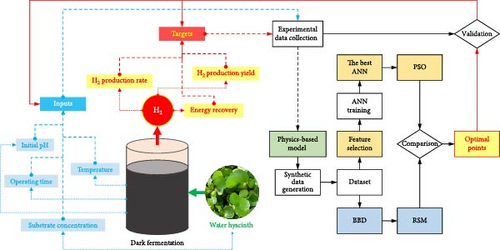
Figure 1 illustrates the sequential study steps to accomplish the aforementioned goals. First, synthetic datasets for the implementation of RSM and ANN training were created through the simulation of the physics-based model of DF@WH. In the ANN training procedure, a variety of ANN topologies were inspected to find the best ANN model. The optimal points were then determined by using the best ANN model’s output as the objective function for the optimization algorithm (i.e., PSO). Ultimately, these optimal points were experimentally validated (details of the experimental procedure can be found in Appendix A, Supporting Information) and compared with the optimization results obtained from RSM. All computational processes in this study were carried out on a desktop computer, which was configured with an Intel Core i7-8700 processor, ran on a Windows 11 operating system, and had 16 GB of DDR4 RAM.

Details are in the caption following the image — **Figure 1**
Open in figure viewer PowerPoint

The workflow for modeling and optimizing dark fermentation fed with water hyacinth (DF@WH) by combining physics-based model and intelligent techniques. ANN, artificial neural network; BBD, Box–Behnken design; H₂, hydrogen; PSO, particle swarm optimization; RSM, response surface methodology.

2.1. Physics-Based Model

Until now, although numerous microorganisms have been found to be able to convert organic material to H₂ via DF (e.g., Clostridium sp., Bacillus sp., and Enterobacter sp.), most studies on DF@WH have used mixed cultures instead of pure cultures [7, 9, 10, 12, 15], as the use of mixed cultures provides more significant economic and technological benefits [36–38]. In the modeling of DF using mixed cultures, the microorganisms are usually considered to be a component or reactant in the system [39–41]. Meanwhile, substrate concentration, initial pH, temperature, and operating time are often selected as basic operating parameters for modeling and optimization [39–41]. In most studies on DF@WH using mixed cultures, the Gompertz model has been widely used to describe H₂ production [7, 8, 13]. Unfortunately, it is not applicable for optimization as the estimated parameters of the Gompertz model are limited to a specific operating condition and, therefore, cannot be extended to other conditions [42].

Recently, a kinetic model, a type of physics-based model, for performance prediction of DF@WH using mixed cultures has been developed by Phan, Phan, and Nguyen [43], which integrated the effect of fundamental operating parameters, such as temperature, initial pH, and substrate concentration. Accordingly, this model was constructed assuming that the WH feedstock exists in two forms (i.e., particulate and soluble) and undergoes two sequential steps (i.e., hydrolysis and acidogenesis) in the DF process. The surface-limiting model [42] and the modified Michaelis–Menten model [44] were used to model the hydrolysis of particulate and soluble forms, respectively. The Luedeking–Piret model [45] was used to model the change rate of H₂ production. Meanwhile, the effects of substrate concentration, operating temperature, and pH were modeled based on the Aiba model [46], the modified Ratkowsky model [47], and the ADM1 model [48], respectively. This model was validated by the literature and experimental data with a high R² value of 0.97 for dark fermentative H₂ production from WH [43]. Therefore, this kinetic model was chosen as a computational experimental dataset generator for this study.

2.2. Dataset Generation

The synthetic dataset was generated by simulating the abovementioned kinetic model in the MATLAB/Simulink software (2023a, MathWorks Inc., USA) using an adaptive algorithm, variable-step type, automatically selected solver, and a relative tolerance of 10⁻⁴. The WH concentration, initial pH, temperature, and operating time were selected as the inputs. The Box–Behnken design (BBD) was chosen as the multilevel experimental design for RSM implementation because of its simplicity and ability to reduce the amount of experiments required [49]. Accordingly, 29 operating condition sets need to be generated for BBD, as illustrated in Table S1 (Supporting Information). On the other hand, to guarantee the ANN training dataset, the studied range for operating parameters of DF@WH comprises an initial pH of 5–8, WH concentration of 5–45 g-TS/L, and temperature of 20–40°C. The maximum operating time was set at 168 h, and the accumulated H₂ volume was recorded every 6 h. With such a setup, a dataset of 9135 operating condition sets needs to be generated. To reduce the dataset size for faster ANN training without loss of information, the PSO-based feature selection [50] was used to select the highest influence data points in a total of 9135 initial data points. The fitness function for feature selection was set based on the mean of the normalized original dataset (i.e., all data points in the original dataset are transformed into their respective values in the range of 0–1). A higher influential data point is determined if its normalized mean is closer to the mean of the normalized original dataset (i.e., 0.445). Different selected data sizes of 1%, 2%, 5%, 8%, and 10% of the original dataset were employed for ANN training. The best ANN models obtained in these procedures were validated with a fixed dataset containing 456 least influential data points (i.e., equivalent to 5% of the original dataset).

2.3. Evaluation Performance of DF@WH

The performance of DF@WH was evaluated through H₂ production yield (HY, mL/g-TS), H₂ production rate (HPR, mL/L/h), and TER (%), calculated as follows:

(1)

(2)

(3)

where the energy of H₂ production (

, kJ/L), substrate energy input (W_s, kJ/L), heat energy input (W_h, kJ/L), operating temperature (W_l, kJ), and mixing energy (W_m, kJ/L) are calculated as Equations (4)–(8), respectively:

(4)

(5)

(6)

(7)

(8)

where

(mL/L) is the accumulated volume of H₂ produced per 1 L of working volume of the DF reactor;

and ΔH_s are energy values of H₂ (i.e., 285.8 kJ/mol [51]) and WH (i.e., 15.6 kJ/g-TS [15]), respectively; C_S (g-TS/L) is the WH concentration; T (°C) is the operation temperature; T_o is the environmental temperature which is assumed as 25°C; c_p is the specific heat capacity, considered as equal to that of water (c_p = 4.186 kJ/kg/°C); ρ is the mass density of DF media, considered as equal to that of water (ρ = 1.0 kg/L); q_mix (W/L) is the stirring power consumed that is needed for mixing 1 L of the reactor’s working volume, which is assumed to be 0.14 W/L [52]; and q_loss (J/h) is the heat loss from the DF reactor walls during each 1 h operating, which is assumed to be 0.5% of W_h.

2.4. Data-Driven Model Development, Comparison, and Optimization

Based on the previous section, it can be seen that the accumulated volume of H₂ production (, mL/L) is a crucial parameter from which other performance parameters (i.e., HY, HPR, and TER) can be determined. Therefore, it was selected as the ANN’s output. Meanwhile, to simplify optimization using RSM, HY, HPR, and TER were selected as the response variables for RSM model development. At the same time, four operating parameters, including WH concentration, initial pH, temperature, and operating time, were selected as the inputs for ANN and RSM models.

2.4.1. ANN Model Development and Optimization by PSO

The trial-and-error approach and the mean square error (MSE) as the objective function were used to evaluate the accuracy of the ANN models. MSE was defined as follows using Equation (9) [26, 53], and the lowest MSE value corresponds to the best ANN model:

(9)

where m is the number of data points and Y_ex and Y_pr are the experimental and predicted data, respectively.

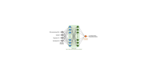
Various ANN structures were examined to ascertain relationships between inputs and outputs using the selected computational dataset (as mentioned in Section 2.2). The training, validating, and testing datasets accounted for 70%, 15%, and 15% of the total divisions of this selected dataset. The hidden layer’s characteristics, including activation functions, the number of hidden layers, and the number of neurons in the hidden layer, were altered to achieve the best ANN. Specifically, several standard activation functions, including logistic sigmoid (logsig), triangular basis (tribas), positive saturating linear (satlin), radial basis (radbas), symmetric saturating linear (satlins), radial basis normalized (radbasn), softmax (softmax), elliot sigmoid (elliotsig), rectified linear unit (ReLU), and hyperbolic tangent (tansig), were sequentially examined. The number of hidden layers and neutrons in each hidden layer was adjusted between 1–3 layers and 1–20 neurons, respectively, as shown in Figure 2. Each ANN topology was trained sequentially using the Deep Learning Toolbox (MATLAB 2023a, MathWorks Inc., USA). The ANN training was stopped when the epoch number reached a maximum of 2000 and/or the gradient value reached a minimum of 10⁻¹². After obtaining the best ANN model, its output (i.e., the accumulated volume of H₂ production) was transformed to HY, HPR, and TER based on Equations (1)–(3) and then considered the objective functions for further optimization by PSO.

The PSO procedure was performed in the Optimize Toolbox (MATLAB 2023a, MathWorks Inc., USA) with the input parameter’s boundaries presented in Table 1. Other parameters of the PSO optimization were kept at the initial setting of the toolbox.

Table 1. Boundaries of input parameters for the optimization procedure.

Parameter	Lower boundary	Upper boundary
WH concentration (g-TS/L)	5	45
Initial pH	5	8
Temperature (°C)	20	40
Operating time (h)	0	168

Abbreviation: WH, water hyacinth.

2.4.2. RSM Model Development and Optimization

The correlation between independent and response variables in the RSM model was described by the second-order polynomial equation, as presented in Equation (10) [54]. The significance of the RSM model was evaluated using an analysis of variance (ANOVA), where a p-value of less than 0.05 was deemed significant. The ANOVA and optimization of RSM were carried out in Design Expert software (version 12.0, Stat-Ease Inc., USA):

(10)

where Y_i represents the response variable (i.e., HY, HPR, and TER); X_i and X_j represent independent variables; and k₀, k_i, k_ij, and k_ij represent the RSM model’s coefficients.

2.4.3. Evaluation and Comparison Between ANN and RSM

In addition to MSE, the coefficient of determination (R²) and normalized root mean squared error (NRMSE) were also used to assess the accuracy of the developed ANN and RSM models. The values of R² and NRMSE were determined as shown in Equations (11) and (12), respectively. In general, the precision of the model increases as the values of R² and NRMSE increase (to a maximum of 1) and decrease (to a minimum of 0), respectively:

(11)

(12)

3. Results and Discussion

3.1. ANN Model Development

Firstly, PSO-based feature selection was implemented to reduce the size of the dataset and thus save time for the ANN training procedure. The effects of various sizes of the selected dataset on the performance of ANN training were presented in Table S2 and Figure S2 (Supporting Information). It can be observed that with a smaller size, the training time was shorter. Specifically, the training time was decreased from 36.2 s for the original dataset to only 2.2 s for the selected dataset’s size of 1%. However, the reduced size also causes a loss of the information of the original dataset, leading to a reduced accuracy of the model. As a result, the size of 5% (i.e., corresponding to 456 data points) can be considered the best size that saved over 75% training time to 8.6 s without changing the information of the original dataset.

Table 2 lists the performance of different ANN models in replicating the kinetic model. Only the most suitable model with the lowest MSE for each activation function is shown here for simplicity. Because of the complexity of DF@WH, it is evident that ANN models with a single hidden layer are insufficient to replicate the outcomes of the kinetic model. Higher hidden layer ANNs, on the other hand, performed better but required more training time because they had a more considerable number of hidden neurons, making them more complex. It is also evident, though, that as the number of hidden layers rose to three, the overcomplexity of these models caused overfitting, which in turn reduced the goodness of fit [55, 56].

Table 2. Summarization of the training performance of various ANN topologies.

Hidden layer number	Activation function	Optimal hidden neuron number	MSE				NRMSE (all)	R² (all)	Training time (s)
Hidden layer number	Activation function	Optimal hidden neuron number	Training	Testing	Validation	All	NRMSE (all)	R² (all)	Training time (s)
1	elliotsig	15	3764.3	14,318.6	4436.0	5451.0	0.0385	0.9868	3.77
	logsig	12	5787.1	11,638.3	8212.8	7030.7	0.0437	0.9830	3.73
	radbas	20	2523.9	10,899.5	8100.6	4620.2	0.0354	0.9888	2.03
	radbasn	20	786.5	8505.5	17,961.5	4526.7	0.0351	0.9890	5.95
	ReLU	16	4911.5	13,692.9	16,338.3	7947.7	0.0465	0.9808	0.58
	satlin	20	5532.0	23,989.0	11,245.4	9163.5	0.0499	0.9778	0.64
	satlins	18	4691.6	5522.4	31,629.5	8863.8	0.0491	0.9786	0.51
	softmax	18	599.2	1283.5	835.0	737.5	0.0142	0.9982	5.13
	tansig	16	2381.5	3251.8	6644.3	3152.7	0.0293	0.9924	4.98
	tribas	19	3693.9	5336.8	16,416.0	5852.2	0.0399	0.9858	0.55

2	elliotsig	16-5	46.4	950.6	1509.9	402.2	0.0105	0.9990	6.46
	logsig	16-8	14.7	24.3	1727.5	273.5	0.0086	0.9993	8.12
	radbas	8-17	145.3	3305.6	7310.8	1696.7	0.0215	0.9959	8.23
	radbasn	19-6	1.4	49.9	394.5	67.8	0.0043	0.9998	9.11
	ReLU	13-11	586.4	2849.2	2919.6	1276.9	0.0186	0.9969	0.63
	satlin	19-9	154.9	722.8	1450.7	434.9	0.0109	0.9989	0.85
	satlins	16-18	275.4	2600.9	6274.1	1526.1	0.0204	0.9963	0.88
	softmax	9-11	42.5	51.4	44.6	44.2	0.0025	0.9999	8.63
	tansig	12-14	19.8	41.4	488.7	93.5	0.0050	0.9997	9.53
	tribas	20-16	2022.7	6076.0	8761.0	3644.1	0.0315	0.9912	1.08

3	elliotsig	9-13-14	604.1	2955.8	1948.8	1159.5	0.0147	0.9972	14.93
	logsig	8-11-19	880.6	1766.4	2700.3	1287.1	0.0139	0.9969	17.07
	radbas	11-12-12	502.1	4444.7	7429.2	2135.2	0.0236	0.9948	14.40
	radbasn	12-16-10	119.2	1318.2	3029.6	736.6	0.0089	0.9982	22.10
	ReLU	9-17-10	1235.1	4475.8	4932.4	2277.5	0.0228	0.9945	1.82
	satlin	11-19-10	961.4	4212.8	2919.9	1744.2	0.0167	0.9958	2.20
	satlins	13-16-10	937.9	3039.1	10,077.4	2626.8	0.0247	0.9936	2.02
	softmax	10-11-13	126.0	236.2	163.2	148.2	0.0042	0.9996	20.07
	tansig	12-14-16	374.0	523.0	1412.0	552.4	0.0087	0.9986	21.05
	tribas	8-14-11	2273.4	5965.1	9909.2	3975.3	0.0327	0.9904	2.37

Note: The boldface represents the best performance.
Abbreviations: ANN, artificial neural network; MSE, mean square error; NRMSE, normalized root mean squared error.

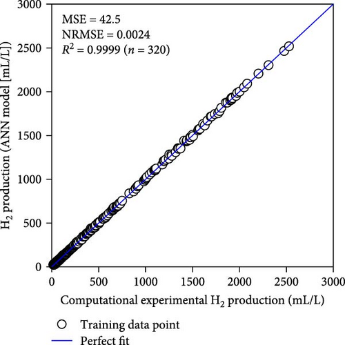
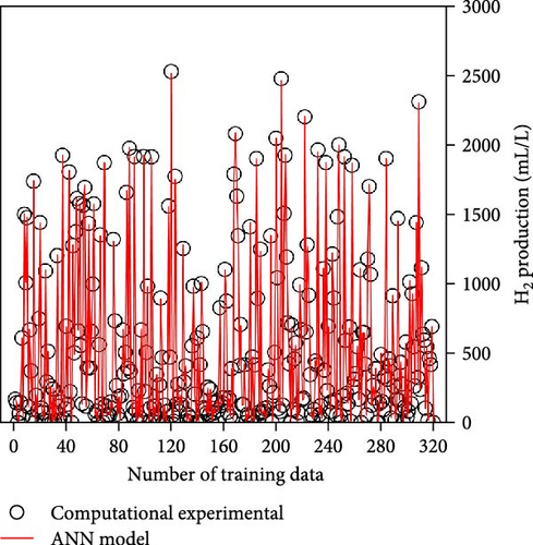
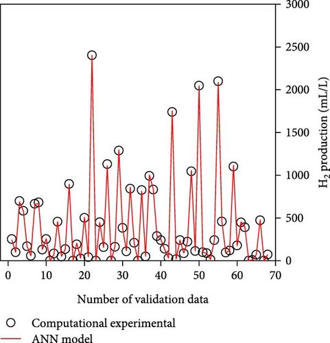
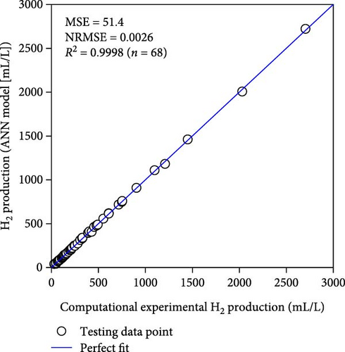
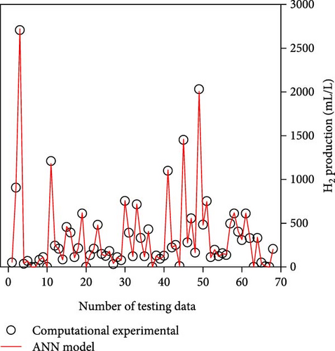
Table 2 demonstrates that the ReLU, tribas, satlins, and satlin functions demonstrated rapid training, taking about 2 s to complete. On the other hand, these activation functions showed subpar performance. In the meantime, the training time and performance of the radbas and radbasn functions were subpar. The elliotsig, tansig, logsig, and softmax functions all required more training time, but their results were superior. With the softmax function and a 4-9-11-1 network topology, the optimal ANN model was thus discovered. With the lowest MSE and NRMSE of 44.2 and 0.0025, respectively, this model demonstrated the best performance. Figure S1 and Table S3 (Supporting Information) provide the specific characteristics of the best ANN model. Furthermore, Figure 3 illustrates that the best ANN model’s expected data were close to the kinetic model-generated synthetic data. All R² values in ANN training, testing, and validation surpass 0.999, indicating the ANN model successfully reproduced the kinetic model.

3.2. Compare to RSM

The expected results from RSM and matching computational synthetic data are shown in Table S4 (Supporting Information). Also, ANOVA results for HY, HPR, and TER responses are presented in Tables S5–S7 (Supporting Information), respectively. The quadratic equation coefficients for these responses in relation to substrate concentration, initial pH, temperature, and operating time are shown in Table S8 (Supporting Information). Consequently, these RSM models were significant based on their high F-values of 4.8–52.9 and low p-values of less than 0.003 [54].

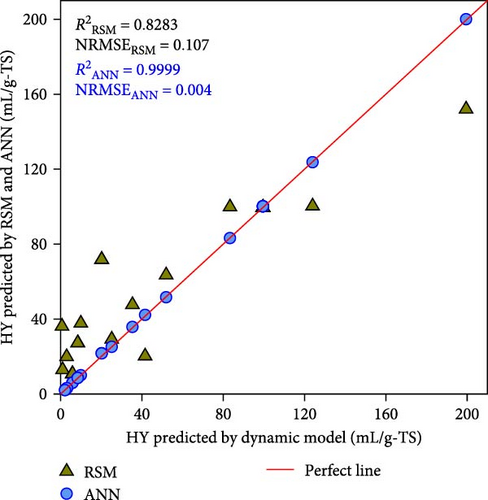
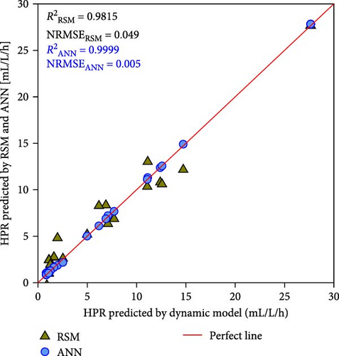
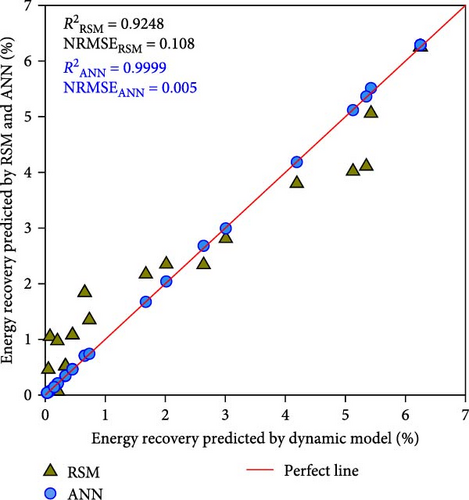
Nevertheless, the RSM models exhibit a substantially lower level of accuracy than the ANN model. Figure 4 shows the correlation between the kinetic model-generated synthetic data and the expected data from the ANN and RSM models. The ANN model demonstrated a predictability that was superior to that of the RSM model, where greater R² values of ≥ 0.9999 were compared to 0.8283–0.9815 of RSM. Besides, compared to the RSM models, the ANN model’s NRMSE values were considerably lower (i.e., 0.004–0.005 vs. 0.049–0.108). In contrast to the RSM, which utilizes a second-order polynomial, the ANN model is able to analyze higher-order nonlinear systems, which accounts for its superior accuracy in terms of predictions [19, 25]. These results once again proved that the best ANN model is reliable for further simulation and optimization.

3.3. ANN Simulation

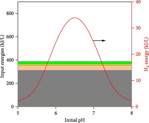
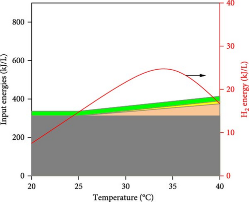
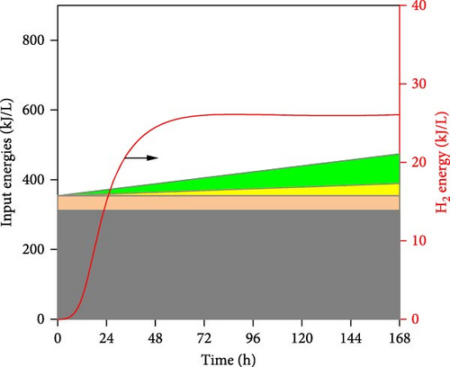
The simulated impacts of WH concentration, temperature, initial pH, and operating time on DF@WH from the best ANN model are shown in Figure 5. Besides, the detailed energies input and output from DF@WH were also simulated and illustrated in Figure 6. These simulation results were obtained under the base conditions of a substrate concentration of 20 g-TS/L, an initial pH of 7.0, a temperature of 35°C, and an operating time of 48 h. It can be observed that the simulation results of the ANN model agreed well with the kinetic model-generated synthetic data. That once again confirms the excellent precision of the ANN model. Moreover, the best ANN model considerably reduced computational time in comparison to the kinetic model. Accordingly, to ensure the data for Figure 5 (i.e., including 50 data points from 22 different operating condition sets), the kinetic model required over 1100 s to simulate; meanwhile, the ANN model only needed less than 2 s to emulate a 15-times-larger dataset (i.e., 750 data points from 330 different operating condition sets).

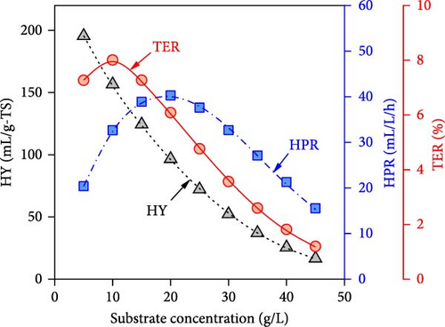
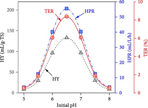
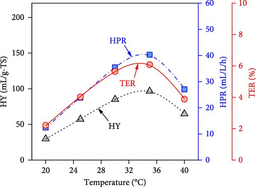
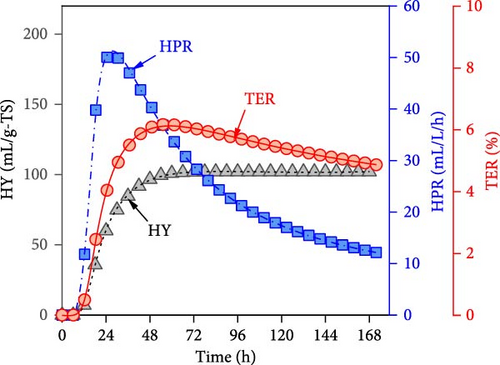
It can be observed in Figure 5 that substrate concentration, initial pH, temperature, and operating time have a multidimensional effect on the energy efficiency and performance of DF@WH. Accordingly, a WH concentration that is too high or too low causes a decline in the performance of DF@WH. As is known, low substrate concentrations cause substrate limitation, while high concentrations lead to substrate inhibition, which reduces hydrolysis and acidogenesis rates [43]. On the other hand, an initial pH and temperature that are too low or too high reduce DF@WH’s productivity and energy efficiency, which are modeled in their inhibition factors [43]. Meanwhile, HY and TER increased in the first 72 h of operation and then changed insignificantly when DF@WH continued to be operated for up to 168 h. This caused a decrease in HPR when the operation time was prolonged.

Figure 6 illustrates the detailed energy output (i.e., H₂ energy) and input into the DF@WH system. It can be seen that the H₂ energy produced tends to be similar to HY since they are both proportional to the cumulative volume of H₂ produced, as illustrated in Equations (1) and (4), respectively. However, it can be observed that this H₂ energy output was significantly lower than the input energies into the DF@WH, which is mainly the energy from the substrate. This is consistent with the results obtained in Figure 5, as increasing substrate concentration significantly reduced the energy conversion efficiency of DF. Besides, except for the effect of initial pH, a change in pH does not change the energy input; increased operating time and temperature increase the energy input requirements associated with heating, heat loss compensation, and agitation. In other words, excessively increasing the substrate concentration, temperature, and operating time increases the input energy, which in turn can reduce the energy recovery of DF@WH. From these simulation results, it is clear that to maximize the performance and efficiency of DF@WH, the substrate concentration, initial pH, temperature, and operating time must be optimized.

3.4. ANN–PSO Optimization

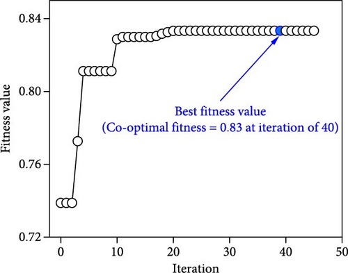
The iteration diagrams and ideal values from the optimization process are displayed in Figure 7. The PSO implementation method showed quick computation; it took roughly 3 s and less than 50 iterations. Such fast calculation of the ANN–PSO approach has also been reported in previous studies [25, 28, 57]. As can also be observed in Figure 7, to achieve the highest performance and efficiency, DF@WH should be operated under an initial pH of 6.5. At the same time, other operational parameters, including substrate concentration, temperature, and operating time, cannot exist at an optimal value to achieve the maximum performance and effectiveness of DF@WH simultaneously. Accordingly, HY could reach the maximum value at 266.8 mL/g-TS when DF was operated at 5.0 g-TS of WH per liter and 34.4°C for 168 h of operation. HPR could be achieved at 80.5 mL/L/h at the WH concentration of 15 g-TS/L, 34.5°C, and after 23.3 h of operation. Meanwhile, to achieve the optimal energy conversion value of 11.4%, DF@WH must be operated at 7.8 g/L, 32.6°C, and for 34 h of operation. These determined optimal conditions are within the typical optimal range previously observed for H₂ production from DF [39, 58, 59].

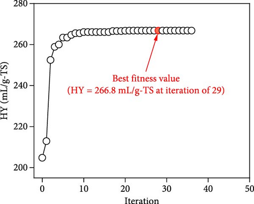
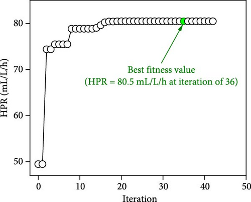
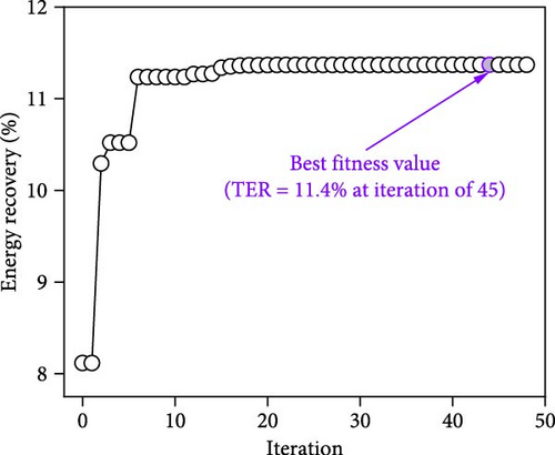
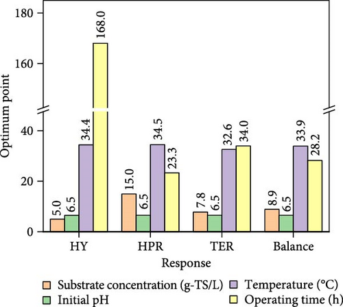
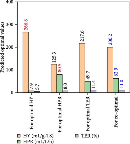
When all performance parameters (i.e., HY, HPR, and TER) were assumed to be of equal importance, the co-optimal conditions for DF@WH were determined at 8.9 g-TS/L of WH, initial pH of 6.5, a temperature of 33.9°C, and operating time of 28.2 h. Under such co-optimal conditions, HY, HPR, and TER could be achieved at 200.2 mL/g-TS, 62.9 mL/L/h, and 11.0%, respectively.

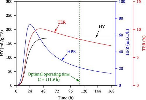
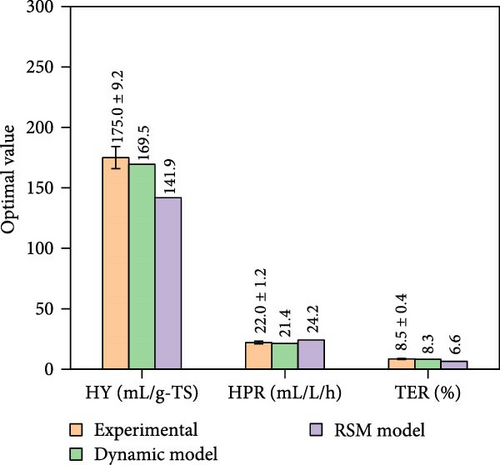
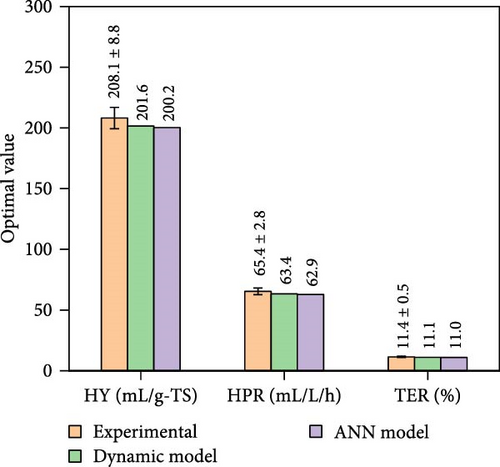
Figure 8 presents the experimental data under co-optimal conditions determined from RSM (i.e., 14.1 g-TS/L, initial pH of 6.5, 31.8°C, and 111.9 h) and ANN–PSO approaches. Additionally, other optimization results of RSM implementation are presented in Table S9 (Supporting Information). It was also found in Figure 8 that the predicted optimal values from RSM were lower and less accurate than the ANN–PSO approach. Specifically, the accuracy of RSM was only 80%–87% and less than 77% when compared to the kinetic model and experimental data, respectively. These values were significantly lower than those from the ANN–PSO approach, with an accuracy of more than 99% compared to the kinetic model and more than 96% compared to the experimental data (details of the experimental procedure can be found in Appendix A, supporting information), reaffirming the precise predictability of the ANN model as well as the ANN–PSO optimization strategy.

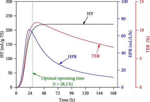
It should be noted that, due to the thermodynamic limit of the DF process, at least two-thirds of the H₂ element are retained in solution to form soluble by-products (such as volatile fatty acids and alcohols) instead of converting turns into H₂ gas [60]. This resulted in low H₂ productivity and energy conversion efficiency of DF@WH. The optimal yield obtained in this study was around 50% higher than the highest value found in the literature (i.e., 134.9 mL/g-TS at 18 g-WH/L, 35°C, initial pH 6, and 24 h of operation [11]). However, it only reached approximately one-fifth of the theoretical H₂ yield of WH (i.e., ~1000 mL/g-TS [12]). Therefore, other downstream processes that can further convert soluble by-products to H₂, such as microbial electrolysis cells and photofermentation, need to be further investigated and optimized. To achieve these goals, further in-depth analyses and simulations of microbial community variation and soluble by-product formation in DF@WH are also required.

4. Conclusion

This study demonstrates that the combined approach of the physics-based model, ANN model, and PSO algorithm is an effective strategy for accurate and rapid simulation and optimization of DF@WH. The simulation results revealed that substrate concentration, initial pH, temperature, and operating time have synergistic effects on DF@WH that must be optimized. The optimization results showed that achieving the highest energy efficiency and performance values at the same time was not possible under a specific optimal operational condition. At co-optimal conditions (i.e., H₂ productivity and TER were seen as being equally significant), the H₂ yield could be achieved at 200.2 mL/g-TS at the production rate of 62.9 mL/L/h with a TER of 11.0%. However, combining DF@WH with other downstream processes, such as microbial electrolysis cells and photofermentation, needs further investigation and optimization to enhance the H₂ productivity and energy recovery from WH.

Conflicts of Interest

The authors declare no conflicts of interest.

Funding

This work was supported by Ho Chi Minh City University of Natural Resources and Environment, Vietnam; Duy Tan University, Vietnam; and Gachon University, South Korea.

Supporting Information

Additional supporting information can be found online in the Supporting Information section.

Open Research

Data Availability Statement

The data that supports the findings of this study are available in the supporting information of this article.

Supporting Information

References

1 Woon J. M., Khoo K. S., and AL-Zahrani A. A., et al.Epitomizing Biohydrogen Production from Microbes: Critical Challenges Vs Opportunities, Environ, Environmental Research. (2023) 227, https://doi.org/10.1016/j.envres.2023.115780, 115780.
10.1016/j.envres.2023.115780
CAS PubMed Google Scholar
2 Tran N., Ta Q. T. H., and Nguyen P. K. T., Transformation of Carbon Dioxide, A Greenhouse Gas, Into Useful Components and Reducing Global Warming: A Comprehensive Review, International Journal of Energy Research. (2022) 46, no. 13, 17926–17951, https://doi.org/10.1002/er.8479.
10.1002/er.8479
CAS Web of Science® Google Scholar
3 Runjavec M. Š., Domanovac M. V., and Jukić A., Application of Industrial Wastewater and Sewage Sludge for Biohydrogen Production, Energies. (2023) 16, no. 5, https://doi.org/10.3390/en16052383, 2383.
10.3390/en16052383
Web of Science® Google Scholar
4 Chen W., Li T., Ren Y., Wang J., Chen H., and Wang Q., Biological Hydrogen With Industrial Potential: Improvement and Prospection in Biohydrogen Production, Journal of Cleaner Production. (2023) 387, https://doi.org/10.1016/j.jclepro.2022.135777, 135777.
10.1016/j.jclepro.2022.135777
CAS Web of Science® Google Scholar
5 Li F., He X., and Srishti A., et al.Water Hyacinth for Energy and Environmental Applications: A Review, Bioresource Technology. (2021) 327, https://doi.org/10.1016/j.biortech.2021.124809, 124809.
10.1016/j.biortech.2021.124809
CAS PubMed Web of Science® Google Scholar
6 Yang E., Chon K., and Kim K. Y., et al.Pretreatments of Lignocellulosic and Algal Biomasses for Sustainable Biohydrogen Production: Recent Progress, Carbon Neutrality, and Circular Economy, Bioresource Technology. (2023) 369, https://doi.org/10.1016/j.biortech.2022.128380, 128380.
10.1016/j.biortech.2022.128380
CAS PubMed Web of Science® Google Scholar
7 Wazeri A., Elsamadony M., Roux S. L., Peu P., and Tawfik A., Potentials of Using Mixed Culture Bacteria Incorporated with Sodium Bicarbonate for Hydrogen Production from Water Hyacinth, Bioresource Technology. (2018) 263, 365–374, https://doi.org/10.1016/j.biortech.2018.05.021, 2-s2.0-85048102573.
10.1016/j.biortech.2018.05.021
CAS PubMed Web of Science® Google Scholar
8 Varanasi J. L., Kumari S., and Das D., Improvement of Energy Recovery From Water Hyacinth by Using Integrated System, International Journal of Hydrogen Energy. (2018) 43, no. 3, 1303–1318, https://doi.org/10.1016/j.ijhydene.2017.11.110, 2-s2.0-85037667260.
10.1016/j.ijhydene.2017.11.110
CAS Web of Science® Google Scholar
9 Varanasi J. L. and Das D., Maximizing Biohydrogen Production From Water Hyacinth by Coupling Dark Fermentation and Electrohydrogenesis, International Journal of Hydrogen Energy. (2020) 45, no. 8, 5227–5238, https://doi.org/10.1016/j.ijhydene.2019.06.030, 2-s2.0-85067877940.
10.1016/j.ijhydene.2019.06.030
CAS Web of Science® Google Scholar
10 Su H., Cheng J., Zhou J., Song W., and Cen K., Hydrogen Production From Water Hyacinth through Dark- and Photo- Fermentation, International Journal of Hydrogen Energy. (2010) 35, no. 17, 8929–8937, https://doi.org/10.1016/j.ijhydene.2010.06.035, 2-s2.0-77956379973.
10.1016/j.ijhydene.2010.06.035
CAS Web of Science® Google Scholar
11 Cheng J., Lin R., Song W., Xia A., Zhou J., and Cen K., Enhancement of Fermentative Hydrogen Production From Hydrolyzed Water Hyacinth With Activated Carbon Detoxification and Bacteria Domestication, International Journal of Hydrogen Energy. (2015) 40, no. 6, 2545–2551, https://doi.org/10.1016/j.ijhydene.2014.12.097, 2-s2.0-84921833576.
10.1016/j.ijhydene.2014.12.097
CAS Web of Science® Google Scholar
12 Cheng J., Xia A., Su H., Song W., Zhou J., and Cen K., Promotion of H₂ Production by Microwave-Assisted Treatment of Water Hyacinth With Dilute H₂SO₄ through Combined Dark Fermentation and Photofermentation, Energy Conversion and Management. (2013) 73, 329–334, https://doi.org/10.1016/j.enconman.2013.05.018, 2-s2.0-84878783815.
10.1016/j.enconman.2013.05.018
CAS Web of Science® Google Scholar
13 Lin R., Cheng J., and Song W., et al.Characterisation of Water Hyacinth With Microwave-Heated Alkali Pretreatment for Enhanced Enzymatic Digestibility and Hydrogen/Methane Fermentation, Bioresource Technology. (2015) 182, 1–7, https://doi.org/10.1016/j.biortech.2015.01.105, 2-s2.0-84922376105.
10.1016/j.biortech.2015.01.105
CAS PubMed Web of Science® Google Scholar
14 Cheng J., Xie B., Zhou J., Song W., and Cen K., Cogeneration of H₂ and CH₄ from Water Hyacinth by Two-Step Anaerobic Fermentation, International Journal of Hydrogen Energy. (2010) 35, no. 7, 3029–3035, https://doi.org/10.1016/j.ijhydene.2009.07.012, 2-s2.0-77951023331.
10.1016/j.ijhydene.2009.07.012
CAS Web of Science® Google Scholar
15 Tran T. T. H. and Nguyen P. K. T., Enhanced Hydrogen Production From Water Hyacinth by a Combination of Ultrasonic-Assisted Alkaline Pretreatment, Dark Fermentation, and Microbial Electrolysis Cell, Bioresource Technology. (2022) 357, https://doi.org/10.1016/j.biortech.2022.127340, 127340.
10.1016/j.biortech.2022.127340
PubMed Web of Science® Google Scholar
16 Sotelo-Navarro P. X. and Poggi-Varaldo H. M., Hydrogen from Dark Fermentation of the Organic Fraction of Waste Diapers: Optimization Based on Response Surface Experiments, Front, Frontiers in Energy Research. (2021) 9, https://doi.org/10.3389/fenrg.2021.630212, 630212.
10.3389/fenrg.2021.630212
Google Scholar
17 Martinez-Burgos W. J., Sydney E. B., and de Paula D. R., et al.Hydrogen Production by Dark Fermentation Using a New Low-Cost Culture Medium Composed of Corn Steep Liquor and Cassava Processing Water: Process Optimization and Scale-Up, Bioresource Technology. (2021) 320, https://doi.org/10.1016/j.biortech.2020.124370, 124370.
10.1016/j.biortech.2020.124370
CAS PubMed Web of Science® Google Scholar
18 Phan T. P., Ta Q. T. H., and Nguyen P. K. T., Maximizing Performance of Microbial Electrolysis Cell Fed With Dark Fermentation Effluent From Water Hyacinth, International Journal of Hydrogen Energy. (2023) 48, no. 14, 5447–5462, https://doi.org/10.1016/j.ijhydene.2022.11.155.
10.1016/j.ijhydene.2022.11.155
CAS Web of Science® Google Scholar
19 Nwosu C., Ayodele O., and Ibrahim H., Optimization of Hydrogen Production via Catalytic Autothermal Reforming of Crude Glycerol Using Response Surface Methodology and Artificial Neural Network, International Journal of Energy Research. (2021) 45, no. 13, 18999–19013, https://doi.org/10.1002/er.7120.
10.1002/er.7120
CAS Web of Science® Google Scholar
20 Nascimento C. A. O., Giudici R., and Guardani R., Neural Network Based Approach for Optimization of Industrial Chemical Processes, Computers & Chemical Engineering. (2000) 24, no. 9-10, 2303–2314, https://doi.org/10.1016/S0098-1354(00)00587-1, 2-s2.0-0034287621.
10.1016/S0098-1354(00)00587-1
CAS Web of Science® Google Scholar
21 Hsu C.-W. and Lin C.-Y., Commercialization Model of Hydrogen Production Technology in Taiwan: Dark Fermentation Technology Applications, International Journal of Hydrogen Energy. (2016) 41, no. 7, 4489–4497, https://doi.org/10.1016/j.ijhydene.2015.07.080, 2-s2.0-84961060157.
10.1016/j.ijhydene.2015.07.080
CAS Web of Science® Google Scholar
22 Buchaniec S., Gnatowski M., and Brus G., Integration of Classical Mathematical Modeling With an Artificial Neural Network for the Problems with Limited Dataset, Energies. (2021) 14, no. 16, https://doi.org/10.3390/en14165127, 5127.
10.3390/en14165127
CAS Web of Science® Google Scholar
23 Bakhtyari A., Mofarahi M., and Iulianelli A., Combined Mathematical and Artificial Intelligence Modeling of Catalytic Bio-Methanol Conversion to Dimethyl ether, Energy Conversion and Management. (2023) 276, https://doi.org/10.1016/j.enconman.2022.116562, 116562.
10.1016/j.enconman.2022.116562
CAS Web of Science® Google Scholar
24 Liu H., Alhumade H., and Elkamel A., A Combined Scheme of Parallel-Reaction Kinetic Model and Multi-Layer Artificial Neural Network Model on Pyrolysis of Reed Canary, Chemical Engineering Science. (2023) 281, https://doi.org/10.1016/j.ces.2023.119109, 119109.
10.1016/j.ces.2023.119109
CAS Web of Science® Google Scholar
25 Yadav S., Singh V., Mahata C., and Das D., Optimization for Simultaneous Enhancement of Biobutanol and Biohydrogen Production, International Journal of Hydrogen Energy. (2021) 46, no. 5, 3726–3741, https://doi.org/10.1016/j.ijhydene.2020.10.267.
10.1016/j.ijhydene.2020.10.267
CAS Web of Science® Google Scholar
26 Le T. H., Thakur D., and Nguyen P. K. T., Modeling and Optimization of Direct Urea-Hydrogen Peroxide Fuel Cell Using the Integration of Artificial Neural Network and Bio-Inspired Algorithms, Journal of Electroanalytical Chemistry. (2022) 922, https://doi.org/10.1016/j.jelechem.2022.116783, 116783.
10.1016/j.jelechem.2022.116783
CAS Web of Science® Google Scholar
27 Nguyen V. T., Ta Q. T. H., and Nguyen P. K. T., Artificial Intelligence-Based Modeling and Optimization of Microbial Electrolysis Cell-Assisted Anaerobic Digestion Fed With Alkaline-Pretreated Waste-Activated Sludge, Biochemical Engineering Journal. (2022) 187, https://doi.org/10.1016/j.bej.2022.108670, 108670.
10.1016/j.bej.2022.108670
CAS Web of Science® Google Scholar
28 Fadlallah S. O., Anderson T. N., and Nates R. J., Artificial Neural Network–Particle Swarm Optimization (ANN-PSO) Approach for Behaviour Prediction and Structural Optimization of Lightweight Sandwich Composite Heliostats, Arabian Journal for Science and Engineering. (2021) 46, no. 12, 12721–12742, https://doi.org/10.1007/s13369-021-06126-0.
10.1007/s13369-021-06126-0
Web of Science® Google Scholar
29 Ming J. L. K., Anuar M. S., How M. S., Noor S. B. M., Abdullah Z., and Taip F. S., Development of an Artificial Neural Network Utilizing Particle Swarm Optimization for Modeling the Spray Drying of Coconut Milk, Foods. (2021) 10, no. 11, https://doi.org/10.3390/foods10112708, 2708.
10.3390/foods10112708
PubMed Web of Science® Google Scholar
30 Vo N. D., Kang J.-H., Oh D.-H., Jung M. Y., Chung K., and Lee C.-H., Sensitivity Analysis and Artificial Neural Network-Based Optimization for Low-Carbon H₂ Production via a Sorption-Enhanced Steam Methane Reforming (SESMR) Process Integrated With Separation Process, International Journal of Hydrogen Energy. (2022) 47, no. 2, 820–847, https://doi.org/10.1016/j.ijhydene.2021.10.053.
10.1016/j.ijhydene.2021.10.053
CAS Web of Science® Google Scholar
31 Vo N. D., Oh D. H., Kang J.-H., Oh M., and Lee C.-H., Dynamic-Model-Based Artificial Neural Network for H₂ Recovery and CO₂ Capture From Hydrogen Tail Gas, Applied Energy. (2020) 273, https://doi.org/10.1016/j.apenergy.2020.115263, 115263.
10.1016/j.apenergy.2020.115263
CAS Web of Science® Google Scholar
32 Ye F., Ma S., Tong L., Xiao J., Bénard P., and Chahine R., Artificial Neural Network Based Optimization for Hydrogen Purification Performance of Pressure Swing Adsorption, International Journal of Hydrogen Energy. (2019) 44, no. 11, 5334–5344, https://doi.org/10.1016/j.ijhydene.2018.08.104, 2-s2.0-85053343797.
10.1016/j.ijhydene.2018.08.104
CAS Web of Science® Google Scholar
33 Sipöcz N., Tobiesen F. A., and Assadi M., The use of Artificial Neural Network Models for CO₂ Capture Plants, Applied Energy. (2011) 88, no. 7, 2368–2376, https://doi.org/10.1016/j.apenergy.2011.01.013, 2-s2.0-79952453396.
10.1016/j.apenergy.2011.01.013
Web of Science® Google Scholar
34 Ochoa-Estopier L. M., Jobson M., and Smith R., Operational Optimization of Crude Oil Distillation Systems Using Artificial Neural Networks, Computers & Chemical Engineering. (2013) 59, 178–185, https://doi.org/10.1016/j.compchemeng.2013.05.030, 2-s2.0-84886382541.
10.1016/j.compchemeng.2013.05.030
CAS Web of Science® Google Scholar
35 Phan T. P., Nguyen T. L., and Nguyen P. K. T., Integrating Physical Knowledge and Artificial Intelligence Approaches for Simulation and Optimization of Direct Urea Fuel Cell, Journal of Electroanalytical Chemistry. (2024) 967, https://doi.org/10.1016/j.jelechem.2024.118493, 118493.
10.1016/j.jelechem.2024.118493
CAS Web of Science® Google Scholar
36 Tran Q. N. and Kim I. T., A Review of Biohydrogen Production from Saccharina Japonica, Fermentation. (2023) 9, no. 3, https://doi.org/10.3390/fermentation9030242, 242.
10.3390/fermentation9030242
CAS Web of Science® Google Scholar
37 Karim A., Islam M. A., Mishra P., Yousuf A., Faizal C. K. M., and Khan M. M. R., Technical Difficulties of Mixed Culture Driven Waste Biomass-Based Biohydrogen Production: Sustainability of Current Pretreatment Techniques and Future Prospective, Renewable and Sustainable Energy Reviews. (2021) 151, https://doi.org/10.1016/j.rser.2021.111519, 111519.
10.1016/j.rser.2021.111519
CAS Web of Science® Google Scholar
38 Mohanakrishna G. and Pengadeth D., Mixed Culture Biotechnology and Its Versatility in Dark Fermentative Hydrogen Production, Bioresour, Bioresource Technology. (2024) 394, https://doi.org/10.1016/j.biortech.2023.130286, 130286.
10.1016/j.biortech.2023.130286
CAS PubMed Google Scholar
39 Boshagh F., Rostami K., and van Niel E. W. J., Application of Kinetic Models in Dark Fermentative Hydrogen Production—A Critical Review, International Journal of Hydrogen Energy. (2022) 47, no. 52, 21952–21968, https://doi.org/10.1016/j.ijhydene.2022.05.031.
10.1016/j.ijhydene.2022.05.031
CAS Web of Science® Google Scholar
40 Yu S., Ryu K., and Lee T., Kinetic Study of pH Effects on Biological Hydrogen Production by a Mixed Culture, Journal of Microbiology and Biotechnology. (2008) 18, 1130–1135.
PubMed Web of Science® Google Scholar
41 Mu Y., Wang G., and Yu H.-Q., Kinetic Modeling of Batch Hydrogen Production Process by Mixed Anaerobic Cultures, Bioresource Technology. (2006) 97, no. 11, 1302–1307, https://doi.org/10.1016/j.biortech.2005.05.014, 2-s2.0-33646398860.
10.1016/j.biortech.2005.05.014
CAS PubMed Web of Science® Google Scholar
42 Kim B., Jeong J., Kim J., Yoon H. H., Nguyen P. K. T., and Kim J., Mathematical Modeling of Dark Fermentation of Macroalgae for Hydrogen and Volatile Fatty Acids Production, Bioresource Technology. (2022) 354, https://doi.org/10.1016/j.biortech.2022.127193, 127193.
10.1016/j.biortech.2022.127193
CAS PubMed Web of Science® Google Scholar
43 Phan Q. H. H., Phan T. P., and Nguyen P. K. T., Mathematical Modeling of Dark Fermentative Hydrogen and Soluble by-Products Generations From Water Hyacinth, Bioresource Technology. (2023) 384, https://doi.org/10.1016/j.biortech.2023.129266, 129266.
10.1016/j.biortech.2023.129266
CAS PubMed Web of Science® Google Scholar
44 Andersen M., Kari J., Borch K., and Westh P., Michaelis—Menten Equation for Degradation of Insoluble Substrate, Mathematical Biosciences. (2018) 296, 93–97, https://doi.org/10.1016/j.mbs.2017.11.011, 2-s2.0-85044603026.
10.1016/j.mbs.2017.11.011
CAS PubMed Web of Science® Google Scholar
45 Wang J. and Wan W., Kinetic Models for Fermentative Hydrogen Production: A Review, International Journal of Hydrogen Energy. (2009) 34, no. 8, 3313–3323, https://doi.org/10.1016/j.ijhydene.2009.02.031, 2-s2.0-64449084684.
10.1016/j.ijhydene.2009.02.031
CAS Web of Science® Google Scholar
46 Aiba S., Shoda M., and Nagatani M., Kinetics of Product Inhibition in Alcoholic Fermentation, Biotechnology and Bioengineering. (1968) 11, 846–864.
Google Scholar
47 Zwietering M. H., de Koos J. T., Hasenack B. E., de Witt J. C., and van’t Riet K., Modeling of Bacterial Growth as a Function of Temperature, Applied and Environmental Microbiology. (1991) 57, no. 4, 1094–1101, https://doi.org/10.1128/aem.57.4.1094-1101.1991.
10.1128/aem.57.4.1094-1101.1991
CAS PubMed Web of Science® Google Scholar
48 Batstone D. J., Keller J., and Angelidaki I., et al.The IWA Anaerobic Digestion Model No 1 (ADM1), Water Science & Technology. (2002) 45, no. 10, 65–73, https://doi.org/10.2166/wst.2002.0292.
10.2166/wst.2002.0292
CAS PubMed Web of Science® Google Scholar
49 Zolgharnein J., Shahmoradi A., and Ghasemi J. B., Comparative Study of Box–Behnken, Central Composite, and Doehlert Matrix for Multivariate Optimization of Pb (II) Adsorption onto Robinia Tree Leaves, Journal of Chemometrics. (2013) 27, no. 1-2, 12–20, https://doi.org/10.1002/cem.2487, 2-s2.0-84874190339.
10.1002/cem.2487
CAS Web of Science® Google Scholar
50 Xue B., Zhang M., and Browne W. N., Particle Swarm Optimisation for Feature Selection in Classification: Novel Initialisation and Updating Mechanisms, Applied Soft Computing. (2014) 18, 261–276, https://doi.org/10.1016/j.asoc.2013.09.018, 2-s2.0-84897113235.
10.1016/j.asoc.2013.09.018
Web of Science® Google Scholar
51 Logan B. E. E., Call D. F. F., and Cheng S., et al.Microbial Electrolysis Cells for High Yield Hydrogen Gas Production from Organic Matter, Environmental Science & Technology. (2008) 42, no. 23, 8630–8640, https://doi.org/10.1021/es801553z, 2-s2.0-57449102625.
10.1021/es801553z
CAS PubMed Web of Science® Google Scholar
52 Suslov D. Y. and Temnikov D. O., Calculation of Energy Costs of Composite Biomass Stirring at Biogas Stations, IOP Conference Series: Materials Science and Engineering. (2018) 327, https://doi.org/10.1088/1757-899X/327/4/042129, 2-s2.0-85046100438, 042129.
10.1088/1757-899X/327/4/042129
Google Scholar
53 Zamaniyan A., Joda F., Behroozsarand A., and Ebrahimi H., Application of Artificial Neural Networks (ANN) for Modeling of Industrial Hydrogen Plant, International Journal of Hydrogen Energy. (2013) 38, no. 15, 6289–6297, https://doi.org/10.1016/j.ijhydene.2013.02.136, 2-s2.0-84877734620.
10.1016/j.ijhydene.2013.02.136
CAS Web of Science® Google Scholar
54 Nguyen P. K. T., Kim J., and Das G., et al.Optimization of Simultaneous Dark Fermentation and Microbial Electrolysis Cell for Hydrogen Production from Macroalgae Using Response Surface Methodology, Biochemical Engineering Journal. (2021) 171, https://doi.org/10.1016/j.bej.2021.108029, 108029.
10.1016/j.bej.2021.108029
CAS Web of Science® Google Scholar
55 Rauh A., Kersten J., Frenkel W., Kruse N., and Schmidt T., Physically Motivated Structuring and Optimization of Neural Networks for Multi-Physics Modelling of Solid Oxide Fuel Cells, Mathematical and Computer Modelling of Dynamical Systems. (2021) 27, no. 1, 586–614, https://doi.org/10.1080/13873954.2021.1990966.
10.1080/13873954.2021.1990966
Web of Science® Google Scholar
56 Wilberforce T. and Olabi A. G., Proton Exchange Membrane Fuel Cell Performance Prediction Using Artificial Neural Network, International Journal of Hydrogen Energy. (2021) 46, no. 8, 6037–6050, https://doi.org/10.1016/j.ijhydene.2020.07.263.
10.1016/j.ijhydene.2020.07.263
CAS Web of Science® Google Scholar
57 Phan T. P., Phan Q. H. H., and Nguyen P. K. T., Dynamic-Based Artificial Intelligence Model for Simulation and Optimization of the Single Chamber Anode Brush Microbial Electrolysis Cell, Fuel. (2024) 375, https://doi.org/10.1016/j.fuel.2024.132629, 132629.
10.1016/j.fuel.2024.132629
CAS Web of Science® Google Scholar
58 Machhirake N. P., Vanapalli K. R., Kumar S., and Mohanty B., Biohydrogen from Waste Feedstocks: An Energy Opportunity for Decarbonization in Developing Countries, Environmental Research. (2024) 252, https://doi.org/10.1016/j.envres.2024.119028, 119028.
10.1016/j.envres.2024.119028
CAS PubMed Web of Science® Google Scholar
59 Zhao Z. T., Ding J., and Wang B. Y., et al.Advances in the Biomass Valorization in Dark Fermentation Systems: A Sustainable Approach for Biohydrogen Production, Chemical Engineering Journal. (2024) 481, https://doi.org/10.1016/j.cej.2023.148444, 148444.
10.1016/j.cej.2023.148444
CAS Web of Science® Google Scholar
60 Dahiya S., Chatterjee S., Sarkar O., Mohan S. V., and Mohan S. V., Renewable Hydrogen Production by Dark-Fermentation: Current Status, Challenges and Perspectives, Bioresource Technology. (2021) 321, https://doi.org/10.1016/j.biortech.2020.124354, 124354.
10.1016/j.biortech.2020.124354
CAS PubMed Web of Science® Google Scholar

Citing Literature

All articles

Combination of Physics-Based Model and Artificial Intelligence for Rapid Simulation and Optimization of Dark Fermentative Hydrogen Production From Water Hyacinth

Abstract

1. Introduction