Recent studies have shown that graph-based clustering methods are good at processing hyperspectral images (HSIs), while falling short for large-scale HSIs due to high time complexity. Meanwhile, the performance of these methods relies on the quality of the constructed graph with selected anchor points. More anchor points bring better clustering results for graph-based methods. Time complexity, however, sees a considerable increase as the number of anchor points grows. Therefore, a method that can obtain efficient clustering accuracy and consumes less time is to be developed. Against this backdrop, a novel algorithm named fast spectral clustering via efficient multilayer anchor graph (FEMAG) is proposed to resolve the accuracy and time-consuming trade-off problem. First, FEMAG adopts superpixel principal component analysis (SuperPCA) to extract the low-dimensional features of HSIs. Then, a multilayer anchor graph is constructed to improve the clustering performance. When constructing the similarity graph, FEMAG takes balanced K-means-based hierarchical K-means (BKHK) to obtain outperforming anchor points efficiently. Extensive experiments validate that FEMAG achieves better clustering accuracy while taking less time compared to previous clustering methods.

1. Introduction

Hyperspectral images (HSIs) record abundant spatial and spectral information with different substances behaving differently at different wavelengths [1–3]. This advantage makes HSIs widely used in environmental monitoring, military detection, and medical diagnosis, among others [4–6]. Abundant information will also introduce redundancy in HSI classification or clustering, and labeled HSIs are labor-consuming work. To solve these issues, scholars tried to bend spatial and spectral information together while reducing the redundancy. For example, a spatial and spectral structure preserved self-representation model for unsupervised hyperspectral band selection without using any label information was proposed by Tang et al. [7] to solve this problem. Clustering analysis, as an unsupervised classification method, can learn the intrinsic similarity of unlabeled samples and divide them into different groups, which is one of the most popular methods in HSI processing [8–10]. According to spectral graph theory, the graph consists of vertices (data points) and edges, where the value of each edge indicates the number of its nearest neighbors [11–13]. Spectral clustering (SC) [14], fast SC [15], and sparse subspace clustering (SSC) [16] are typical graph-based clustering methods.

Graph-based clustering methods have great potential in HSI processing, which exploits the nonlinear pairwise similarity by data distances [17, 18]; therefore, scholars have made deep research on it and made great progress. For instance, Tang et al. [19] proposed unsupervised feature selection via multiple graph fusion and feature weight learning to optimize the quality of the similarity graph. Cai and Chen [20] proposed the landmark-based spectral clustering (LSC) method to get points of higher quality with K-means. Based on this, Huang et al. [21] presented the ultrascalable spectral clustering (U-SPEC) method, in which a fast approximation method with k-nearest representatives is used to construct the sparse affinity submatrix. Wang et al. [22] proposed scalable graph–based clustering with nonnegative relaxation (SGCNR) for large-scale HSIs to reduce the time complexity with stable accuracy.

With these advantages and progress, graph-based clustering methods, however, are faced with huge time consumption challenges in large-scale HSIs because the step of graph construction takes a lot of time due to the huge number of data points [23, 24]. To solve this accuracy and time-consuming trade-off problem, the multilayer anchor graph scheme is introduced in this paper. The clustering performance of the single-layer anchor graph relies heavily on the number and quality of selected anchors. To be specific, more anchors will facilitate the clustering results but cost too much time, which will do nothing good for fast clustering. Too-limited anchors accelerate the clustering speed but may miss important information in the original HSI. In this case, a multilayer graph scheme is considered to grasp key information in the data while boosting the clustering process. Based on the anchor graph method, multiple layers are constructed with decreasing anchors layer by layer while ensuring the correlation between data points. Therefore, a novel algorithm for large-scale HSIs is proposed, which is named fast spectral clustering via efficient multilayer anchor graph (FEMAG). The main contributions of this paper and algorithm are threefold:

1.
FEMAG constructs an anchor-based multilayer anchor graph to get higher accuracy and lower computing cost.
2.
To thoroughly investigate the spatial information of HSI, low-dimensional features are learned by SuperPCA. The computing burden, therefore, has been effectively alleviated.
3.
The parameter-free strategy is applied to achieve self-adaptive optimization of the heat-kernel parameter.

2. Overview of Graph-Based SC

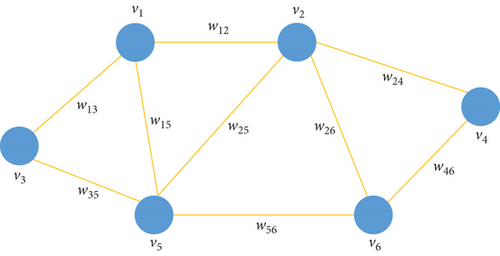
In graph-based theory, each data point (a pixel in the HSI) is viewed as a vertex, so we let G = {V, ξ, W} be a weighted graph without directions, where V denotes the set of vertexes and ξ denotes the set of edges describing the similarity of one-to-one vertexes. W = [w_ij] ∈ ℝ^n×n is the similarity matrix of the graph, which can be obtained by Gaussian function , where ‖•‖₂ is defined by Euclidean distance between vectors and σ is the heat-kernel parameter, whose value has a direct impact on clustering performance and needs to be tuned manually in experiments. See the weighted graph in Figure 1.

Details are in the caption following the image — **Figure 1**
Open in figure viewer PowerPoint

Illustration of a weighed graph without directions.

For HSIs, denotes the data matrix, where n is the number of data points and d represents the dimension of the image.

3. Description of FEMAG Algorithm

Key steps of the FEMAG algorithm are as follows: (1) use SuperPCA to reduce the redundant information in an HSI so as to lighten the computation burden; (2) construct a multilayer anchor graph to better describe the relationship between data points while decreasing the time complexity; and (3) adopt balanced K-means-based hierarchical K-means (BKHK) to select the most representative anchors to increase the clustering efficiency.

3.1. Low-Dimensional Feature Generation With SuperPCA Algorithm

Principal component analysis (PCA) is known as an effective preprocessing step for HSIs. Following recent studies on PCA [25], we adopt the efficient algorithm SuperPCA to obtain low-dimensional features of HSI data. SuperPCA includes two main steps:

1.
Performing superpixel segmentation on initial HSI data according to the entropy rate of superpixels.
2.
Implementing PCA on smaller components and rearranging the obtained low-dimensional matrix to compose the reduced-dimensional data.

Recently, graph-based methods have been widely adopted for superpixel segmentation [26, 27]. According to spectrogram theory, constructing a graph G = (ξ, ζ) with edge set ξ and vertices set ξ. ξ consists of the pairwise similarities by the weight function ζ⟶ℝ⁺ ∪ {0}. In [28], an entropy rate superpixel segmentation method is proposed to group an HSI into several subgraphs. Therefore, we define the subset of edges as A⊆ξ. Moreover, the objective function of the entropy rate superpixel is defined as

()

where O(A) is an entropy rate term and B(A) is a balancing term, while α is used to balance the contributions of O(A) and B(A). According to [29], we can use an effective greedy method to achieve the optimization of Equation (1).

To process HSI more efficiently, the SuperPCA algorithm needs to convert the original d-dimensional HSI data

into

-dimensional space

, where

. To ensure generality, we can be defined as follows:

()

where P denotes the transformation matrix. Then, by solving the following objective function, the linear transformation matrix P can be found.

()

where cov(X) is the covariance of the matrix X. The dimension-reduced HSIs can be formed by extracting the same number of principal components for each homogeneous region. Then, PCA is used to reduce the dimensions.

3.2. Anchor Generation With BKHK

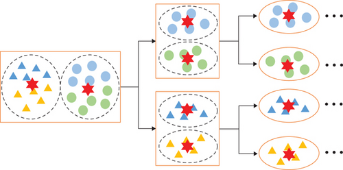
Anchor-based methods select m anchor points from n data points in the image, where m ≪ n. Several ways, such as random selection, K-means, and the BKHK algorithm [30, 31], are used to obtain anchor points. The random selection is simple and fast but fails to select good enough to construct the similarity graph. K-means can generate more representative anchors, but its time complexity is too high, making it hard to apply for large-scale HSI. BKHK segments data into two clusters with the same number iteratively and thus can select representative anchor points efficiently, which is suitable for large-scale HSIs. In this paper, we adopt BKHK to get brilliant anchors efficiently. Figure 2 demonstrates the schematic of the BKHK algorithm. Triangles and circles indicate raw data points, and different colors represent different categories. The red hexagon is the cluster center, and the BKHK algorithm generates data points for each layer by balanced K-means.

3.3. The Parameter-Free Anchor-Based Similarity Matrix

The similarity between data points and anchor points is measured by matrix Z, in which the element z_ij means the adjacency between the i-th data point and j-th anchor point, z_ij can be defined as follows [32]:

()

where Φ ⊂ {1, 2, ⋯, m} denotes the indexes of the k_-nearest neighbors of y_i in U. K( ) represents a kernel function, where Gaussian kernel is widely adopted.

()

where σ is the heat-kernel parameter, which needs time-consuming tuning in experiments. To tackle this problem, we obtain the i-th row of Z in Equation (4) by solving the following problem:

()

where

denotes the j-th row of Z and γ is a regularization parameter. For convenience, the square of Euclidean distance between a data point and an anchor point is marked as

. From Reference [33], we could know that z_i is sparse with k nonzero values, and thus the matrix Z is also sparse. According to Equation (6), we get the optimal affinities z_ij as follows:

()

where k is the number of nearest neighbors. The essence of Equation (7) lies in selecting a small set of anchor points to capture the whole feature of the image.

3.4. Multilayer Anchor Graph Construction

The interlayer adjacency relationship needs to be described to construct the multilayer anchor graph. Suppose the bottom layer (H₀) denotes the original HSI data

, the other layers (H_a, a = 1, 2, ⋯, h) are composed of several anchor matrix

, where m_a is the number of points in H_a. The size of U_a is gradually reduced. Let Z_H denote the similarity between H₀_, and Z_H can be also expressed as

()

Suppose F_h is the class indicator of H_h, F₀ is the class indicator matrix of the original data points in H₀. By accumulating matrices, we can get the class indicator matrix from H₀ to H_h in a sparse manner:

()

As Z_H is got, the similarity matrix W can be obtained by [22]:

()

where

is the diagonal matrix and

. As we obtain the similarity matrix W, the Laplacian matrix L then can be obtained by

()

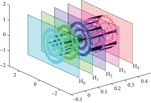
To provide a vivid description, the multilayer anchor graph is shown in Figure 3. In each layer, there are three-ring synthetic data, and the original layer H₀ consists of 4000 data points. Then, K-means is used to select the following layers with H₁ = 2000, H₂ = 1000, H₃ = 500, and H₄ = 250 anchor points.

3.5. The FEMAG Algorithm

From Equation (11), the objective function of FEMAG is defined as

()

The cost function can be written as

()

where λ is the regularization parameter. Then, taking the derivative of Equation (13) about F and setting it to zeros, we have LF^∗ = λF^∗. The optimal solution is the eigenvalue decomposition on L whose time complexity is O(n²c), which is too high to deal with large-scale HSI clustering. W is automatically normalized, and the degree matrix D = I, where I denotes the identity matrix. According to Equation (10), the similarity matrix W can be written as W = MM^T, where

. Then perform singular value decomposition (SVD) on E to get the solution of Equation (12) while reducing the time complexity to O(nm_hc). The SVD of E can be written as follows:

()

where Q ∈ ℝ^n×n, Σ ∈ ℝ^n×m, and V ∈ ℝ^m×m are the left singular vector matrix, singular value matrix, and right singular vector matrix, respectively. It is verified that the column vectors of Q are the eigenvectors of W = MM^T. The SVD of the matrix M obtained the relaxed continuous solution, which is composed of eigenvectors corresponding to the smallest c eigenvalues. Here, we apply the K-means to discretize the solution.

The time complexity of FEMAG can be approximated as .

To express the method more clearly, the detailed FEMAG is described in Table 1.

Table 1. The FEMAG algorithm.

Step	Details
Input	HSI data matrix X ∈ ℝ^n×d; the number of superpixels s; the reduced dimension ; the number of neighbors k; and the number of anchor points m₁, m₂, ⋯m_h
Output	The class indicator c
Step 1	Extract low-dimensional features of original data by SuperPCA
Step 2	Generate anchor points by BKHK
Step 3	Get matrix Z_0,1Z_1,2 ⋯ Z_h−1,h according to Equation (7)
Step 4	Achieve matrix Z_H according to Equation (8)
Step 5	Obtain matrix W according to Equation (10)
Step 6	Get the related continuous solution of F by conducting SVD on matrix M
Output	Obtain the class indicator by K-means

4. Experiments

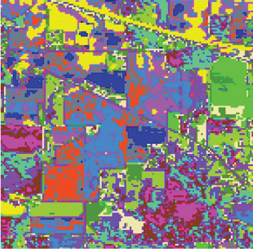
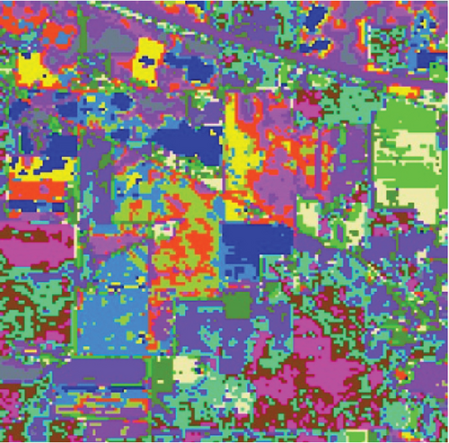
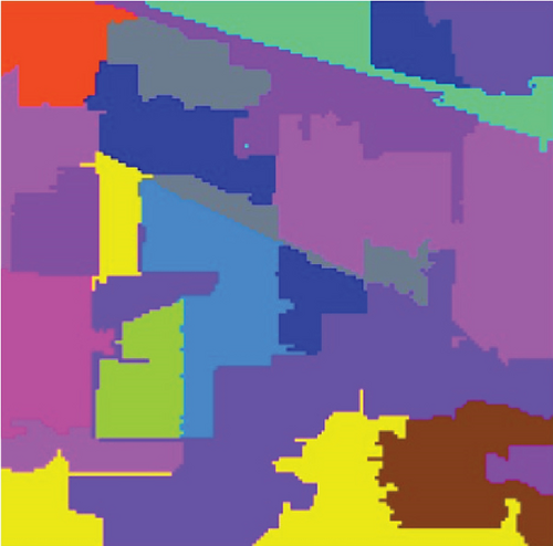
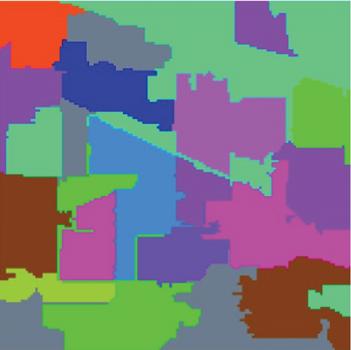
In this section, the HSI data sets used in experiments and the parameter setting are introduced at the beginning. To confirm the performance of FEMAG, we compare it with classic SC methods (named SC [34], LSC-R, LSC-K, U-SPEC, and SGCNR). FEMAG selects anchor points by random and K-means, respectively, marked as FEMAG-R and FEMAG-K. Then, the clustering time of different methods is analyzed. All the experiments are implemented on three open HSI data sets, Indian Pines (Figure 4), Salinas (Figure 5), and Pavia Center (Figure 6) by a PC with Intel i9-10980XE (36) @ 4.60GHz and 64-GB RAM, MATLAB 2021a.

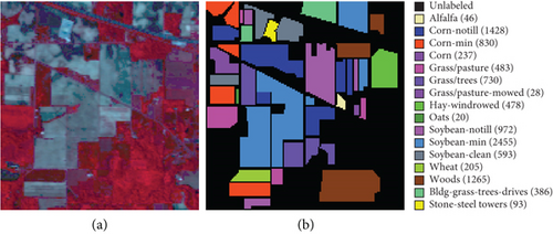
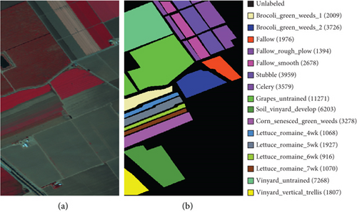
In the experiments, Indian Pines is regarded as a small-sized data set, Salinas as a medium-sized one, and Pavia Center as a large-sized. Both clustering maps and index evaluations are provided to demonstrate the efficiency and effectiveness of FEMAG. Quantitative evaluations adopt the user’s accuracy (UA), average accuracy (AA), overall accuracy (OA), and kappa coefficient. Besides, the best clustering results are highlighted in boldface.

For clarity, we use FEMAG-m₁, m₂, ⋯, m_h to denote the FEMAG method with h layer anchor graph. For example, FEMAG-512-256 means that there are two anchor layers in its graph structure, containing 512 and 256 anchor points, respectively. Moreover, FEMAG-m means the FEMAG contains m anchor points; for example, FEMAG-1024 means that the FEMAG contains 1024 anchor points.

4.1. Parameter Sensitivity

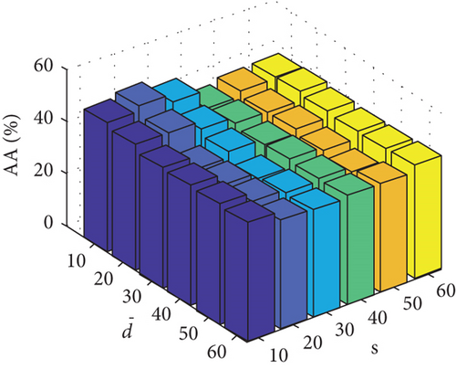
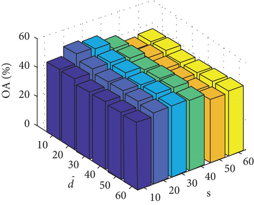
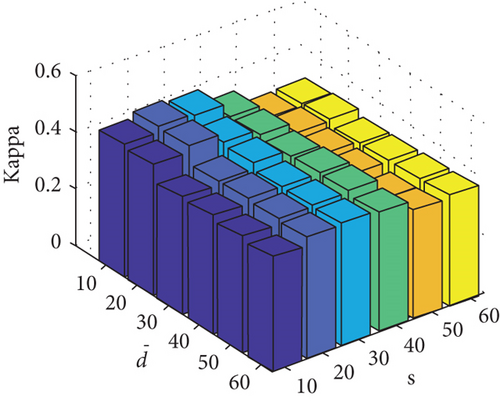
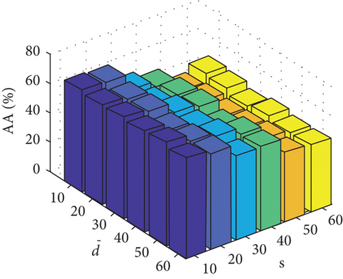
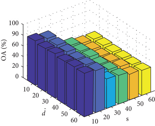
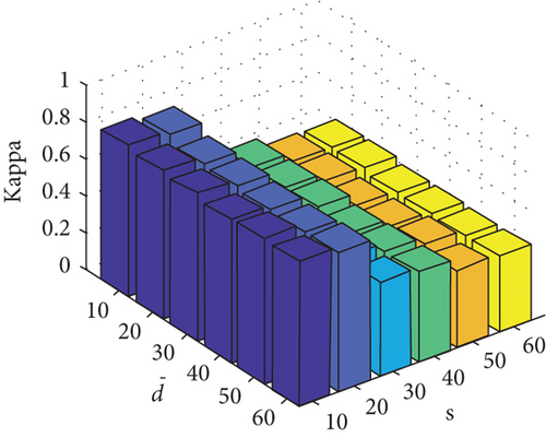
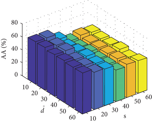
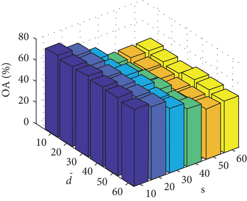
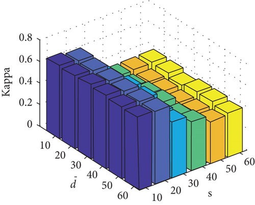
In this section, the parameter sensitivity of FEMAG will be assessed. SuperPCA includes three parameters: s, , and k. The clustering performance is mainly affected by s and ; k is related to the sparsity of matrix Z and has little effect on the time complexity.

Parameter sensitivity experiments are conducted on the three HSI data sets. By referring to Figures 7(a), 7(b), and 7(c), we see that the clustering performance depends mainly on the parameter s, and the parameter has little effect on the clustering performance. Note that the motivation of our FEMAG algorithm is efficient, it is reasonable to select a small s = 20 and for Indian Pines data set. Figures 7(d), 7(e), and 7(f) show that the clustering performance of FEMAG is relatively robust to parameter , noting that parameter s = 10 is the best performance achieved by the FEMAG algorithm. As shown in Figure 7(g), FEMAG is quite insensitive to with wide ranges of values. In terms of OA and kappa, we get similar observations. The result validates the above analysis. The smaller s can obtain better clustering results in the joint action.

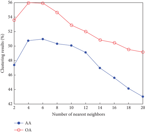
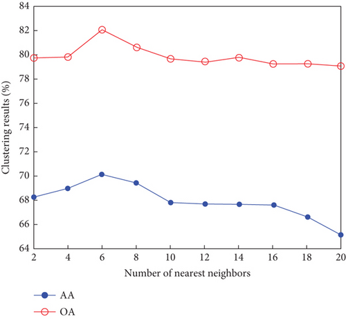
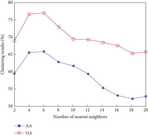
Finally, the sensitivity of parameter k involved in FEMAG is tested. For convenience, k varies from 2 to 20, and the corresponding results are shown in Figure 8, from which we can see that as a general trend, the clustering results become worse with the increase of the number of nearest neighbors and k < 10 making the result reasonable on the three HSI data sets. Therefore, it is acceptable to set k = 5.

A multilayer anchor graph is constructed in FEMAG for better clustering performance; therefore, it is a key point how sensitive the algorithm is to the layers of the anchor graph. Extensive experiments are conducted to test it, and the clustering results are shown in Tables 2, 3, and 4.

Table 2. The FEMAG with different layers and anchors in the Indian Pines data set.

Method	F-64	F-128	F-256	F-512	F-128-64	F-256-128	F-256-128-64	F-512-256-128
AA (%)	38.61	43.72	46.67	48.57	44.74	50.15	51.54	53.27
OA (%)	52.41	54.49	48.16	54.30	53.95	55.12	57.21	62.37
Kappa	0.4610	0.4847	0.4329	0.4843	0.4823	0.5086	0.5215	0.5801
Time (s)	0.6	0.8	1.1	1.9	0.8	1.5	2.1	3.0

Note: The best clustering results are highlighted in boldface.

Table 3. The FEMAG with different layers and anchors in the Salinas data set.

Method	F-64	F-128	F-256	F-512	F-128-64	F-256-128	F-256-128-64	F-512-256-128
AA (%)	60.30	62.46	64.72	67.13	65.19	68.31	69.85	73.12
OA (%)	72.36	74.17	75.58	75.12	79.60	82.53	82.22	82.56
Kappa	0.6871	0.7082	0.7253	0.7224	0.7722	0.8052	80.08	80.49
Time (s)	2.6	4.1	7.2	10.5	6.8	9.10	10.64	12.1

Note: The best clustering results are highlighted in boldface.

Table 4. The FEMAG with different layers and anchors in the Pavia Center data set.

Method	F-128	F-256	F-512	F-1024	F-256-128	F-512-256	F-512-256-128	F-1024-512-256
AA (%)	55.53	58.03	61.30	64.54	61.27	65.52	65.86	66.89
OA (%)	73.22	73.22	74.85	75.77	74.40	76.63	76.79	77.56
Kappa	0.6341	0.6354	0.6517	0.6758	0.6523	0.6802	0.6941	0.7012
Time (s)	23.8	33.7	42.5	52.7	36.5	48.50	55.68	63.7

Note: The best clustering results are highlighted in boldface.

From the left four columns of Table 2, it can be seen that as the number of anchor points grows, the FEMAGs with a single layer see increasing clustering accuracy (AA, OA, and kappa coefficient) and the same trend with the clustering time.

From the right two columns, it is clear that FEMAG with three layers, such as F-256-128-64 and F-512-256-128, has higher clustering accuracy with more anchor points. The AA, OA, and kappa have increased by 3.4%, 9.0%, and 11.2%, respectively, while the clustering time has also grown from 1.5 to 3.0 s, which is still acceptable.

Experiments have also been done in the Salinas and Pavia Center data sets and obtained the same conclusions.

These experiments and results illustrate that the number of layers and anchors depends on the real application requirements. The selection of layer number is to strike the balance between time complexity and clustering accuracy. For example, if high clustering accuracy is required while the clustering speed is tolerated, a more layer with a large amount of anchor point graph can be constructed; if HIS clustering needs to be completed in a short period of time and the accuracy requirement is not very high, then a less layer with less anchor point graph can be constructed to finish a fast clustering.

4.2. Small-Size Data Set

To evaluate the performance of clustering methods on small-size data, experiments are first conducted on the Indian Pines. For this small data set, we construct the anchor graph with 256 and 128 anchor points in FEMAG, written as FEMAG-256-128. The parameters of the FEMAG are set as k = 5, s = 20, and . In addition, the number of anchor points of algorithms LSC-R, LSC-K, U-SPEC, and SGCNR is set to 128 during the experiment.

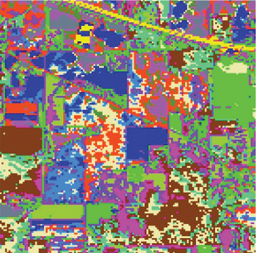
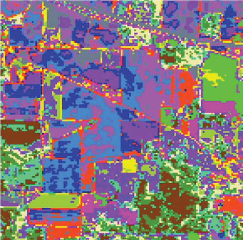
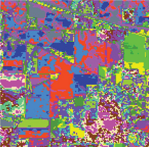
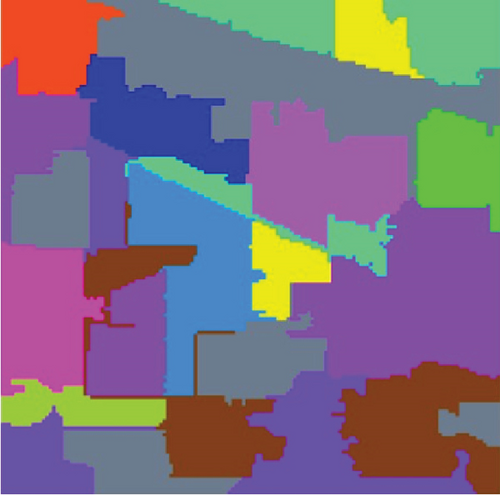
The clustering maps shown in Figure 9 and the corresponding evaluations and time consumed in Table 5 show that LSC-R gets unsatisfying clustering results incorporating numerous misclassifications, with the lowest OA of 31.26% and kappa coefficient of 0.2549. LSC-K and FEMAG-K perform better by significantly decreasing the misclassifications and improving by almost 4% and 11% in AA compared to randomly selected anchor points. Three graph-based clustering methods—LSC-K, U-SPEC, and SGCNR—obtain better clustering performance than SC.

Table 5. Quantitative evaluation on the Indian Pines data set.

Class	SC	LSC-R	LSC-K	U-SPEC	SGCNR	FEMAG-R	FEMAG-K	FEMAG
Alfalfa	0	0	0	10.87	0	0	0	0
Corn-notill	44.05	26.75	25.14	32	30.25	63.17	43.77	43.77
Corn-mintill	33.13	21.45	30.6	33.98	31.33	31.93	31.93	31.93
Corn	12.24	14.77	25.74	17.3	27.43	22.78	75.95	75.95
Grass-pasture	24.64	49.9	35.82	49.48	50.1	65.84	12.01	65.84
Grass-trees	30.41	47.95	44.52	34.52	53.70	60.27	60.27	39.73
Grass-pasture-mowed	0	92.86	0	32.14	0	0	0	3.57
Hay-windrowed	82.01	18.83	92.47	93.72	99.37	0	100.00	100.00
Oats	0	0	55	45	0	0	0	0
Soybean-notill	23.87	24.18	29.84	30.25	27.06	82.00	82.00	82.00
Soybean-mintill	24.52	28.8	29.98	30.88	31.28	43.99	43.99	43.99
Soybean-clean	16.86	27.15	21.42	22.43	16.69	64.59	64.59	96.29
Wheat	96.1	96.1	97.56	96.1	96.59	0	99.51	99.51
Woods	55.65	40.4	34.94	34.86	29.09	42.92	42.92	42.92
Buildings-grass-trees-drives	19.69	16.06	19.69	18.65	22.8	76.94	76.94	76.94
Stone-steel-towers	59.14	31.18	52.69	0	77.42	0	0	0
AA (%)	32.64	33.52	37.21	36.39	37.07	34.65	45.87	50.15
OA (%)	35.44	31.26	34.59	35.49	36.32	49.56	52.2	55.12
Kappa	0.2969	0.2549	0.2872	0.2907	0.3009	0.4427	0.4762	0.5086
Time (s)	38.0	1.4	2.3	0.8	10.1	1.0	3.7	1.5

Note: The best clustering results are highlighted in boldface.

As is shown in Table 5, the FEMAG obtains the highest accuracy with an AA of 50.15%, which is 4.28%~17.51% higher than the FEMAG-R and FEMAG-K algorithms. For OA and kappa, the accuracies obtained by FEMAG are 55.12% and 0.5086, which are 2.92%~23.86% and 0.0324~0.2537 higher than FEMAG-R and FEMAG-K. For the eight classes of corn, grass-pasture, hay-windrowed, soybean-notill, soybean-mintill, soybean-clean, wheat, and buildings-grass-trees-drive, FEMAG obtains the highest precision of 75.95%, 65.84%, 100%, 82%, 43.99%, 96.29%, 99.51%, and 76.94%. The running times of LSC-R, LSC-K, U-SPEC, FEMAG-R, FEMAG-K, and FEMAG belong to the same order of magnitude.

4.3. Medium-Sized Data Set

For the Salinas data set, a three-layer anchor graph with 256, 128, and 64 anchor points is constructed in FEMAG, marked as FEMAG-256-128-64. In addition, the parameters of FEMAG are set as k = 5, s = 10, and . The number of anchor points of algorithms LSC-R, LSC-K, U-SPEC, and SGCNR is set to 256 during the experiment.

Table 6 shows the quantitative evaluations and running time, and Figure 10 shows the clustering maps, from which we can see that FEMAG obtains better clustering maps and produces more homogenous areas compared with other algorithms. It is obvious that FEMAG-K and FEMAG obtain better clustering performance than FEMAG-R, which fully shows that K-means and BKHK can select more representative anchor points. In addition, we can also draw this conclusion from the LSC algorithm.

Table 6. Quantitative evaluations on the Salinas data set.

Class	LSC-R	LSC-K	U-SPEC	SGCNR	FEMAG-R	FEMAG-K	FEMAG
Brocoliweeds_1	0	99.70	98.36	98.41	100.00	100.00	100.00
Brocoliweeds_2	65.59	40.77	54.32	81.51	99.92	99.84	99.54
Fallow	44.38	25.76	23.48	20.65	0	0	0
Fallowrough	99.71	98.78	99.86	96.92	99.28	99.78	99.57
Fallowsmooth	90.93	88.87	92.87	65.50	98.70	98.36	98.77
Stubble	96.64	98.81	97.73	93.74	97.30	99.57	99.67
Celery	53.20	99.30	99.39	99.41	99.92	99.92	99.92
Grapesuntrained	43.62	43.92	57.99	59.13	45.63	86.60	86.58
Soil	80.27	66.79	84.59	87.47	99.95	99.94	99.95
Corn	58.63	60.22	9.82	63.67	1.07	0.7	21.38
Lettuce_4wk	73.60	81.74	23.6	66.76	0	0	0
Lettuce_5wk	13.70	44.47	91.90	63.47	0	100	100.00
Lettuce_6wk	98.03	99.13	97.49	99.45	0	0	0
Lettuce_7wk	87.48	0	92.15	0	0	0	0
Vinyarduntrained	42.23	38.00	60.26	60.04	85.65	99.35	99.30
Vinyardtrellis	18.65	17.87	0	0.17	98.84	96.29	88.32
AA (%)	60.41	62.76	67.74	66.02	57.89	67.52	68.31
OA (%)	57.24	59.20	66.80	68.70	67.57	81.55	82.53
Kappa	0.5326	0.5553	0.6306	0.6528	0.6454	0.7943	0.8052
Times (s)	3.6	5.3	4.7	60.3	5.4	39.3	48.5

Note: The best clustering results of each material are highlighted in boldface.

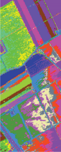
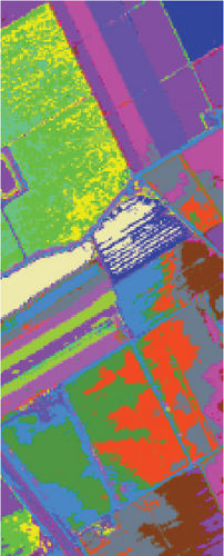
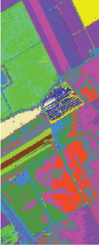
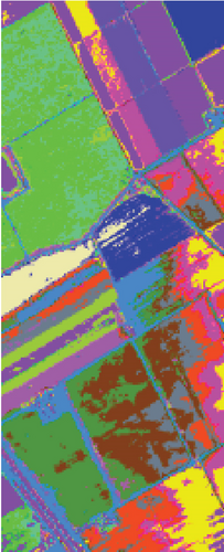
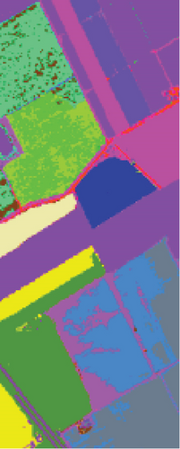
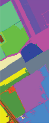
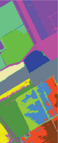
As seen in Table 6, the FEMAG outperforms other methods with AA of 68.31%, OA of 82.53%, and kappa of 0.8052, which are 0.79%~7.9%, 0.98%~25.23%, and 0.0109~0.2726 higher than other methods. It can also be seen that FEMAG-R, FEMAG-K, and FEMAG generate smoother clustering results than LSC-R in this scene, with the 10.33%, 24.31%, and 25.29% improvement in OA. The running time of LSC-R, LSC-K, U-SPEC, FEMAG-R, and FEMAG is of the same order of magnitude. In particular, the FEMAG only takes 9.1 s, which is six and four times faster than the SGCNR and FEMAG-K, respectively. Note that SC cannot work on the Salinas data set due to an “out of memory (OM)” error because the Salinas data set has 111,104 pixels (samples) whose size is too large for SC.

4.4. Large-Sized Data Set

To demonstrate that FEMAG can perform well on large-sized HSI data, experiments on the Pavia Center data set are implemented. We construct a two-layer anchor graph with 512 and 256 anchor points in FEMAG, marked as FEMAG-512-256. In addition, the parameters of FEMAG are set as follows: k = 5, s = 10, and . Then, the number of anchor points in algorithms LSC-R, LSC-K, U-SPEC, and SGCNR is set to 256.

The clustering maps of the Pavia Center data set are shown in Figure 11, which shows that FEMAG achieved the best clustering results; meanwhile, FEMAG, FEMAG-K, and SGCNR obtained smoother clustering maps than other algorithms by taking spatial information into account.

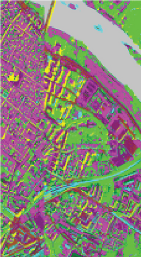
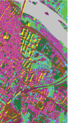
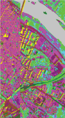
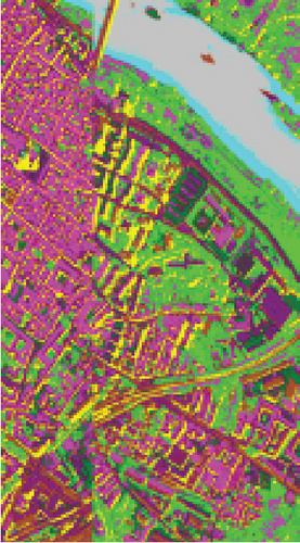
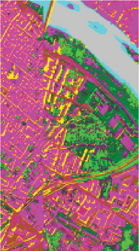
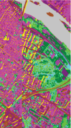
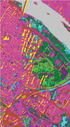
By referring to Table 7, FEMAG obtains the highest precision with the best AA of 65.52%, increased by 4%~15% than other competitors; its OA is 76.63%, increased by 2.5%~9.8% than other competitors; and kappa coefficient of 0.6802, which has increased by 3.2%~13.9%. The performance of FEMAG is better than FEMAG-R and FEMAG-K, which is attributed to the effectiveness of the BKHK algorithm and anchor-based graph construction strategy. Water and asphalt classes are effectively distinguished, and the recognition level is much higher than that of other methods.

Table 7. Quantitative evaluations on the Pavia Center data set.

Class	LSC-R	LSC-K	U-SPEC	SGCNR	FEMAG-R	FEMAG-K	FEMAG
Water	98.55	98.7	98.97	90.04	90.01	96.51	99.56
Trees	99.8	69.01	75.89	72.11	56.25	54.11	23.22
Asphalt	0	9.06	10.49	0	0	1.2	49.39
Self-blocking bricks	0.19	96.35	0	67.64	58.96	58.36	58.77
Bitumen	54.42	39.66	30.59	26.22	61.33	48.56	48.6
Tiles	81.53	84.69	82.96	71.27	88.89	75.58	88.57
Shadows	55.78	1.3	61.04	76.45	19.49	65.12	65.82
Meadows	43.76	56.66	52.49	63.09	50.6	44.38	55.9
Bare soil	99.9	99.86	99.9	99.93	99.9	99.9	99.86
AA (%)	59.33	61.7	56.92	62.97	58.38	60.41	65.52
OA (%)	73.84	74.84	74.82	74.56	69.82	71.67	76.63
Kappa	0.6484	0.6589	0.6551	0.6576	0.5974	0.6204	0.6802
Times (s)	23.4	28.2	12.7	129.2	25.3	241.5	48.5

Note: The best clustering results of each line are highlighted in boldface.

The table shows that the running times of LSC-R, LSC-K, U-SPEC, FEMAG-R, and FEMAG are 23.4, 28.2, 12.7, 25.3, and 48.5 s, respectively. As the scale of the data set grows, the total number of samples increases to 783640 in the Pavia Center data set. Focus on six graph-based clustering methods, FEMAG needs 48.5 s, and SC cannot work on it due to “OM error.” Since the anchor-graph and BKHK strategies are adopted, the graph construction is rather fast, and the clustering performance is also relatively outstanding.

5. Conclusion

The performance of clustering methods is based on anchor graphs as well as how anchors are selected. To tackle the problem, we proposed the FEMAG algorithm. First, SuperPCA learns the intrinsic low-dimensional features of HSIs. Second, a multilayer anchor graph is constructed, which can effectively reduce the time complexity while better describing the relationship between pixels and anchors. Third, other than the K-means method, BKHK can select anchors much faster. Experimental results demonstrate that FEMAG with BKHK is 3.4 times faster than FEMAG with K-means, and the OA of FEMAG is 20.1%~44.2% higher than other methods, which means FEMAG significantly outperforms state-of-art methods.

Conflicts of Interest

The authors declare no conflicts of interest.

Author Contributions

Yiwei Wei and Chao Niu designed the research. Dejun Liu and Peinan Ren modified the draft.

Funding

This study was financially supported by the National Natural Science Foundation of China (No. 52272446).

Acknowledgments

This study was financially supported by the National Natural Science Foundation of China (No. 52272446).

Open Research

Data Availability Statement

The data that support the findings of this study are available from the corresponding author upon reasonable request.

References

1 Xue Z., Du P., Li J., and Su H., Sparse graph regularization for hyperspectral remote sensing image classification, IEEE Transactions on Geoscience and Remote Sensing. (2017) 55, no. 4, 2351–2366, https://doi.org/10.1109/TGRS.2016.2641985, 2-s2.0-85009875935.
10.1109/TGRS.2016.2641985
Google Scholar
2 Wu X., Hong D., and Chanussot J., Convolutional neural networks for multimodal remote sensing data classification, IEEE Transactions on Geoscience and Remote Sensing. (2022) 60, 1–10, https://doi.org/10.1109/TGRS.2021.3124913.
10.1109/TGRS.2021.3124913
Web of Science® Google Scholar
3 He F., Wang R., and Jia W., Fast semi-supervised learning with anchor graph for large hyperspectral images, Pattern Recognition Letters. (2020) 130, 319–326, https://doi.org/10.1016/j.patrec.2018.08.008, 2-s2.0-85051557817.
10.1016/j.patrec.2018.08.008
Google Scholar
4 Jakob S., Zimmermann R., and Gloaguen R., The need for accurate geometric and radiometric corrections of drone-borne hyperspectral data for mineral exploration: MEPHySTo - a toolbox for pre-processing droneborne hyperspectral data, Remote Sensing. (2017) 9, no. 1, https://doi.org/10.3390/rs9010088, 2-s2.0-85010676775.
10.3390/rs9010088
Google Scholar
5 Khan M. J., Khan H. S., Yousaf A., Khurshid K., and Abbas A., Modern trends in hyperspectral image analysis: a review, IEEE Access. (2018) 6, 14118–14129, https://doi.org/10.1109/ACCESS.2018.2812999, 2-s2.0-85043766341.
10.1109/ACCESS.2018.2812999
Web of Science® Google Scholar
6 Zhong Y., Ma A., and Zhang L., An adaptive memetic fuzzy clustering algorithm with spatial information for remote sensing imagery, IEEE Journal of Selected Topics in Applied Earth Observations and Remote Sensing. (2014) 7, no. 4, 1235–1248, https://doi.org/10.1109/JSTARS.2014.2303634, 2-s2.0-84899940849.
10.1109/JSTARS.2014.2303634
Web of Science® Google Scholar
7 Tang C., Wang J., Zheng X., and Xie W., Spatial and spectral structure preserved self-representation for unsupervised hyperspectral band selection, IEEE Transactions on Geoscience and Remote Sensing. (2023) 61, 1–13, https://doi.org/10.1109/TGRS.2023.3331236.
10.1109/TGRS.2023.3331236
Google Scholar
8 Jain A. K., Data clustering: 50 years beyond k-means, Pattern Recognition Letters. (2010) 31, no. 8, 651–666, https://doi.org/10.1016/j.patrec.2009.09.011, 2-s2.0-77950369345.
10.1016/j.patrec.2009.09.011
Web of Science® Google Scholar
9 Hong D., Gao L., Yao J., Zhang B., Plaza A., and Chanussot J., Graph convolutional networks for hyperspectral image classification, IEEE Transactions on Geoscience and Remote Sensing. (2021) 59, no. 7, 5966–5978, https://doi.org/10.1109/TGRS.2020.3015157.
10.1109/TGRS.2020.3015157
Web of Science® Google Scholar
10 Yang X., Xu Y., Li S., Liu Y., and Liu Y., Fuzzy embedded clustering based on bipartite graph for large-scale hyperspectral image, IEEE Geoscience and Remote Sensing Letters. (2022) 19, 1–5, https://doi.org/10.1109/LGRS.2021.3073035.
10.1109/LGRS.2021.3073035
CAS Web of Science® Google Scholar
11 Zhang H., Zhai H., Zhang L., and Li P., Spectral-spatial sparse subspace clustering for hyperspectral remote sensing images, IEEE Transactions on Geoscience and Remote Sensing. (2016) 54, no. 6, 3672–3684, https://doi.org/10.1109/TGRS.2016.2524557, 2-s2.0-84959892702.
10.1109/TGRS.2016.2524557
Web of Science® Google Scholar
12 Wu Z. and Leahy R. M., An optimal graph theoretic approach to data clustering: theory and its application to image segmentation, IEEE Transactions on Pattern Analysis and Machine Intelligence. (1993) 15, no. 11, 1101–1113, https://doi.org/10.1109/34.244673, 2-s2.0-0027697605.
10.1109/34.244673
Web of Science® Google Scholar
13 Prades J., Safont G., Salazar A., and Vergara L., Estimation of the number of endmembers in hyperspectral images using agglomerative clustering, Remote Sensing. (2020) 12, no. 21, https://doi.org/10.3390/rs12213585.
10.3390/rs12213585
Google Scholar
14 Pacella M. and Papadia G., Fault diagnosis by multisensor data: a data-driven approach based on spectral clustering and pairwise constraints, Sensors. (2020) 20, no. 24, https://doi.org/10.3390/s20247065, 33321733.
10.3390/s20247065
PubMed Google Scholar
15 Chen G. and Lerman G., Spectral curvature clustering (SCC), International Journal of Computer Vision. (2009) 81, no. 3, 317–330, https://doi.org/10.1007/s11263-008-0178-9, 2-s2.0-58149494138.
10.1007/s11263-008-0178-9
Web of Science® Google Scholar
16 Wang R., Nie F., and Yu W., Fast spectral clustering with anchor graph for large hyperspectral images, IEEE Geoscience and Remote Sensing Letters. (2017) 14, no. 11, 2003–2007, https://doi.org/10.1109/LGRS.2017.2746625, 2-s2.0-85030635040.
10.1109/LGRS.2017.2746625
Web of Science® Google Scholar
17 Yang X., Lin G., Liu Y., Nie F., and Lin L., Fast spectral embedded clustering based on structured graph learning for large-scale hyperspectral image, IEEE Geoscience and Remote Sensing Letters. (2022) 19, 1–5, https://doi.org/10.1109/LGRS.2020.3035677.
10.1109/LGRS.2020.3035677
CAS Web of Science® Google Scholar
18 Kang Z., Wen L., Chen W., and Xu Z., Low-rank kernel learning for graph-based clustering, Knowledge-Based Systems. (2019) 163, 510–517, https://doi.org/10.1016/j.knosys.2018.09.009, 2-s2.0-85054058394.
10.1016/j.knosys.2018.09.009
Web of Science® Google Scholar
19 Tang C., Zheng X., Zhang W., Liu X., Zhu X., and Zhu E., Unsupervised feature selection via multiple graph fusion and feature weight learning, Science China Information Sciences. (2023) 66, no. 5, article 152101, https://doi.org/10.1007/s11432-022-3579-1.
10.1007/s11432-022-3579-1
Google Scholar
20 Cai D. and Chen X., Large scale spectral clustering via landmark-based sparse representation, IEEE Transactions on Cybernetics. (2015) 45, no. 8, 1669–1680, https://doi.org/10.1109/TCYB.2014.2358564, 2-s2.0-85027924713, 25265642.
10.1109/TCYB.2014.2358564
PubMed Web of Science® Google Scholar
21 Huang D., Wang C., Wu J., Lai J., and Kwoh C., Ultra-scalable spectral clustering and ensemble clustering, IEEE Transactions on Knowledge and Data Engineering. (2020) 32, no. 6, 1212–1226, https://doi.org/10.1109/TKDE.2019.2903410, 2-s2.0-85063010130.
10.1109/TKDE.2019.2903410
Web of Science® Google Scholar
22 Wang R., Nie F., Wang Z., He F., and Li X., Scalable graph-based clustering with nonnegative relaxation for large hyperspectral image, IEEE Transactions on Geoscience and Remote Sensing. (2019) 57, no. 10, 7352–7364, https://doi.org/10.1109/TGRS.2019.2913004.
10.1109/TGRS.2019.2913004
Web of Science® Google Scholar
23 Yang X., Yu W., Wang R., Zhang G., and Nie F., Fast spectral clustering learning with hierarchical bipartite graph for large-scale data, Pattern Recognition Letters. (2020) 130, 345–352, https://doi.org/10.1016/j.patrec.2018.06.024, 2-s2.0-85050530100.
10.1016/j.patrec.2018.06.024
Web of Science® Google Scholar
24 Liu W., He J., and Chang S., Large graph construction for scalable semi-supervised learning, Proceedings of the 27th international conference on machine learning (ICML-10), 2010, Haifa, Israel, 679–686.
Google Scholar
25 Yang X., Liu G., Yu Q., and Wang R., Stable and orthogonal local discriminant embedding using trace ratio criterion for dimensionality reduction, Multimedia Tools and Applications. (2018) 77, no. 3, 3071–3081, https://doi.org/10.1007/s11042-017-5022-1, 2-s2.0-85024491233.
10.1007/s11042-017-5022-1
Web of Science® Google Scholar
26 Nascimento M. C. V. and De Carvalho A. C., Spectral methods for graph clustering - a survey, European Journal of Operational Research. (2011) 211, no. 2, 221–231, https://doi.org/10.1016/j.ejor.2010.08.012, 2-s2.0-79951677261.
10.1016/j.ejor.2010.08.012
Google Scholar
27 Jiang J., Ma J., Chen C., Wang Z., Cai Z., and Wang L., SuperPCA: a superpixelwise PCA approach for unsupervised feature extraction of hyperspectral imagery, IEEE Transactions on Geoscience and Remote Sensing. (2018) 56, no. 8, 4581–4593, https://doi.org/10.1109/TGRS.2018.2828029, 2-s2.0-85048767391.
10.1109/TGRS.2018.2828029
Web of Science® Google Scholar
28 Verdoja F. and Grangetto M., Fast superpixel-based hierarchical approach to image segmentation, Image Analysis and Processing—ICIAP 2015: 18th International Conference, Genoa, Italy, September 7-11, 2015, Proceedings, Part I 18, 2015, Springer International Publishing, 364–374.
10.1007/978-3-319-23231-7_33
Google Scholar
29 Iyer G., Chanussot J., and Bertozzi A. L., A graph-based approach for data fusion and segmentation of multimodal images, IEEE Transactions on Geoscience and Remote Sensing. (2021) 59, no. 5, 4419–4429, https://doi.org/10.1109/TGRS.2020.2971395.
10.1109/TGRS.2020.2971395
Google Scholar
30 Liu M., Tuzel O., Ramalingam S., and Chellappa R., Entropy rate superpixel segmentation, CVPR 2011, 2011, Colorado Springs, CO, USA, 2097–2104, https://doi.org/10.1109/CVPR.2011.5995323, 2-s2.0-80052896536.
10.1109/CVPR.2011.5995323
Google Scholar
31 Nemhauser G. L., Wolsey L. A., and Fisher M. L., An analysis of approximations for maximizing submodular set functions - I, Mathematical Programming. (1978) 14, no. 1, 265–294, https://doi.org/10.1007/BF01588971, 2-s2.0-0000095809.
10.1007/BF01588971
Web of Science® Google Scholar
32 He F., Nie F., Wang R., Hu H., Jia W., and Li X., Fast semi-supervised learning with optimal bipartite graph, IEEE Transactions on Knowledge and Data Engineering. (2021) 33, no. 9, 3245–3257, https://doi.org/10.1109/TKDE.2020.2968523.
10.1109/TKDE.2020.2968523
Google Scholar
33 Zhu W., Nie F., and Li X., Fast spectral clustering with efficient large graph construction, 2017 IEEE International Conference on Acoustics, Speech and Signal Processing (ICASSP), 2017, New Orleans, LA, USA, 2492–2496, https://doi.org/10.1109/ICASSP.2017.7952605, 2-s2.0-85023745957.
10.1109/ICASSP.2017.7952605
Google Scholar
34 Li Y., Nie F., Huang H., and Huang J., Large-scale multi-view spectral clustering via bipartite graph, Proceedings of the AAAI Conference on Artificial Intelligence. (2015) 29, no. 1, 2750–2756, https://doi.org/10.1609/aaai.v29i1.9598.
10.1609/aaai.v29i1.9598
Google Scholar

All articles

Fast Spectral Clustering via Efficient Multilayer Anchor Graph

Abstract

1. Introduction

2. Overview of Graph-Based SC

3. Description of FEMAG Algorithm