Comparison of Machine Learning and Classic Methods on Aerodynamic Modeling and Control Law Design for a Pitching Airfoil
Abstract
Aerodynamic modeling and control law design methods are crucial foundational technologies that enable efficient maneuvering flight of aircraft. Hence, this study focuses on how to construct the aerodynamic model and design control law using machine learning, as well as their differences from classical methods. To conduct this, a modified NACA0012 airfoil with a tail functioning as an elevator is employed as the geometry model. Through the utilization of the rigid dynamic grid method and overlapping grid technology, the pitch of the airfoil and the deflection of the elevator are efficient to execute. Firstly, the pitching moment coefficient is sampled through both steady and unsteady computations. Then, multivariate nonlinear regression (MNR) models and artificial neural network (ANN) models are established based on steady and unsteady sampling data, respectively. Additionally, the obtained model is evaluated using open-loop control laws. Based on the evaluation, the proportional-integral-derivative (PID) control algorithm is used to design the airfoil pitching control law using the MNR model. Meanwhile, deep reinforcement learning (DRL) is used to design the pitching control law using the ANN model. Finally, the PID and DRL controllers are implemented in a CFD environment for airfoil pitching control to verify their effectiveness in application scenarios. The results suggest that models based on both steady and unsteady data can reflect dynamic aerodynamic characteristics. However, using unsteady computation for data sampling significantly reduces time consumption compared to steady computation. Furthermore, the model constructed by ANN may have unexpected excellent characteristics. Both the PID and DRL control laws, designed based on the models, perfectly complete the control process in the CFD environment. This study provides valuable insights for the implementation of controllable maneuvering flight in aircraft.
1. Introduction
A century ago, humanity achieved the awe-inspiring feat of piloting flight into the sky with aircraft, after overcoming challenges of power and controllability, thus ushering in a magnificent era of aviation. Even today, ensuring safe and efficient flight remains a crucial focus, requiring extensive research on the stability and control characteristics of aircraft [1]. Furthermore, to achieve outstanding maneuverability such as fighters, a reliable and efficient flight control system is indispensable. Adequate attention is given to the research of aerodynamic modeling technology and the control law design method as they hold utmost significance in this pursuit.
To achieve controllable flight of an aircraft, several steps need to be followed. Firstly, the aerodynamic data of the aircraft must be obtained. This data is then used to establish an aerodynamic model, which serves as the basis for designing the control law. Afterward, the control law is developed by incorporating the aerodynamic model and relevant algorithms. Subsequently, the control law is applied to the aircraft for test flights, and corrections and compensations are made based on the results. Finally, the control law is implemented for the general flight of the aircraft. Traditionally, aerodynamic data is obtained through wind tunnel tests [2]. With advancements in high-performance computing and numerical methods, computational fluid dynamics (CFD) has emerged as an alternative way of obtaining aerodynamic data [3]. CFD can be classified as steady or unsteady computation, depending on the time correlation. Most previous studies have utilized steady computations due to their ability to provide high-precision data that meets research needs. In addition, obtaining aerodynamic data is to establish an aerodynamic model. This is because designing control laws based on aerodynamic models can effectively reduce costs. Because the model is essentially a reduced order processing method during flowing, it can effectively retain the main information. For example, the proper orthogonal decomposition is a commonly used reduced-order method for analyzing flow structure [4, 5], and multivariate nonlinear regression (MNR) methods can be used to establish aerodynamic models. In the field of flight control, conventional methods such as proportional-integral-derivative (PID) control still dominate. Chen et al. [6] designed a PID controller based on the transfer function established using aerodynamic data. They assessed the accuracy of the flight control system by comparing the performance of the controller in engineering simulations and CFD coupling simulations. Allan et al. [7] proposed a trimming algorithm for longitudinal control of aircraft. This algorithm incorporates trimmer operators within a feedback loop using a dual time-stepping scheme, and they demonstrated the effectiveness of this algorithm in achieving longitudinal maneuvering using a standard model. Zhang et al. [8] established a model using a steady aerodynamic database. Based on this model, they applied the nonlinear dynamic inversion method to conduct numerical virtual flight (NVF) research on missile pitch control. In addition, they also performed a validation study of the missile’s pitch controlled by PID using a NVF system along with wind tunnel virtual flight testing [9]. Overall, obtaining accurate aerodynamic data, developing suitable control laws, and refining them based on test flight results are integral steps in realizing controllable flight for aircraft. The advancements in CFD and the utilization of traditional control methods, such as PID, have played significant roles in this process.
However, the method of obtaining aerodynamic data through steady computation is relatively inefficient. To establish a reliable aerodynamic model, it is necessary to set up multiple sampling points within the range of flight parameters. Furthermore, each computation can only yield data for one specific state point. This significantly increases the overall computation cost and hampers the development and iterative design of aircraft prototypes. Additionally, the aircraft’s attitude is frequently adjusted dynamically during flight, making the flow turbulent and resulting in the unsteady and nonlinear effect of aerodynamics [10]. The application of the MNR method requires prior determination of the polynomial structure, therefore requiring multiple attempts or relying heavily on the experience of researchers. In terms of control, classic PID control methods can achieve stable and efficient control within linear fields. Nevertheless, modern aircraft often operate under highly complex conditions, sometimes in nonlinear fields. Therefore, to ensure flight safety, redundant designs are required with the cost of sacrificing some aircraft performance. Overall, there is an urgent need to develop more efficient methods for aerodynamic data collection, as well as related modeling techniques and more advanced “smart” control methods.
To tackle the aforementioned challenges, researchers have transcended the confines of conventional methodologies. For instance, the application of population-based genetic algorithms has been instrumental in addressing aerodynamic optimization issues, yielding remarkable outcomes [11, 12]. In recent years, artificial intelligence (AI) has emerged as a prominent area of research, especially with the recent growth of the foundation model leading to what is seen by many as a new wave of technological revolution [13]. Machine learning (ML) [14], as a quintessential example of AI, has found wide-ranging applications in various fields [15]. Notably, in the domains of aerospace and aerodynamics, there has been an increasing number of reports highlighting the impact of ML in these areas [16, 17]. It has been empirically demonstrated that this technology cannot only match but also surpass the effectiveness of traditional methodologies. For example, Wang et al. [18] presented a novel vortex identification method based on ML. Similarly, Yi and Cheng. [19] investigated the optimal design and flow mechanism of a high-pressure ratio impeller with ML. Furthermore, Li, Zhang, and Chen [20] employed deep reinforcement learning (DRL) to successfully design supercritical airfoils. In a different study, Rabault et al. [21] employed an artificial neural network (ANN) trained by DRL to discover active control strategies for flow around a cylinder.
In the application of ML to aircraft aerodynamic modeling and flight control, there have been some relevant literature reports [22], although the number remains limited. In the early stages, Punjani and Abbeel [23] utilized deep learning to develop a dynamics model for a real aerobatic helicopter, while Bansal et al. [24] also explored the use of neural networks in quadrotor dynamics flight control. More recently, Liang et al. [25] integrated an ANN with a PID controller for adaptive control of a missile in the field of numerical simulation, resulting in significant advancements. Xu, Tian, and Xia [26] also demonstrated impressive outcomes. They established multiple sampling points for unsteady data sampling and utilized a deep neural network to establish the aerodynamic model. Based on this foundation, DRL was employed to achieve an effective control process.
Different from the above approaches, this work adopts a simpler and more effective method for sampling aerodynamic data and follows a comprehensive strategy to achieve aerodynamic control, encompassing initial data acquisition, modeling, control law design, and their applications. To demonstrate the feasibility of these novel ideas, classical methods are also taken into consideration for comparison. First, data is sampled using both steady and unsteady methods. Then, MNR models along with ANN models are individually established using the collected aerodynamic data. Based on these models, the PID and DRL methods are applied to design the pitch control law. Subsequently, the control law is tested in a CFD-based NVF [8] environment, yielding excellent results that validate the feasibility of this idea. In the current era of AI development, ML will continue to accelerate progress in intelligence within the realm of aeronautics and aerodynamics.
The remainder of this paper is organized as follows. Section 2 introduces the numerical methods, including primarily the geometric model, computational grid, governing equations, and ML methods employed in the study. Section 3 validated the reliability of the solver through comparison with experiments. Section 4 entails the results and discussion, elaborating on the implementation of both classical methods and ML for aerodynamic modeling and control processes. Finally, the conclusion and remark of this paper are presented in Section 5.
2. Numerical Methods
2.1. Geometric Model and Computational Grid
The focus of this work is to compare the performance of ML methods and traditional methods in aerodynamic modeling and control law design, so a simplified geometry is designed. The geometric model is modified from the well-known symmetrical airfoil NACA0012, as illustrated in Figure 1. The chord length of the airfoil, denoted as c, measures 1 m. To generate the pitching moment, the tail is severed to act as an elevator. The elevator center of rotation is positioned at 75% of the chord length from the nose along the centerline. Moreover, the rotation center of the entire airfoil is situated at 25%c from the nose. At this point, the moment of inertia of the airfoil is 1000 kg•m2.

The computational grid consists of two parts: the main wing grid and the tail grid. The main wing grid occupies a discrete region between the main wing wall and the outer boundary of the circular computational domain. To eliminate the influence of the far field, the outer boundary radius is extended to 25 times the chord length. On the other hand, the tail grid is constructed by filling the tail wall and a portion of the surrounding area. The height of the first layer of the two grids is 1.0 × 10⁻⁶ m. Two grids are combined by an overlapping zone as shown in Figure 2. During pitch maneuver, the main wing grid is rotated using the rigid dynamic grid method. Simultaneously, the tail grid is deflected around its rotating point by the overlapping grid approach and remains synchronized with the movement of the main wing [27].
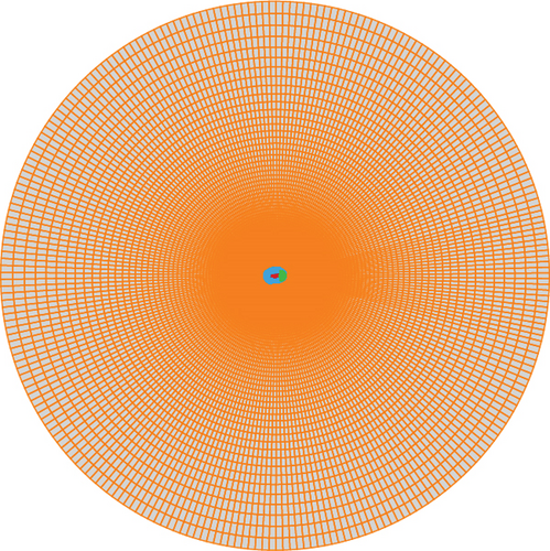
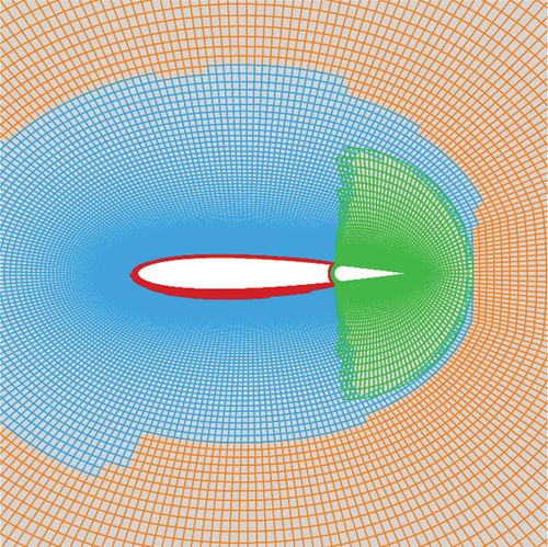
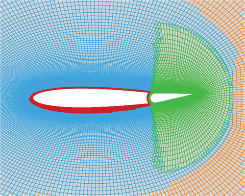
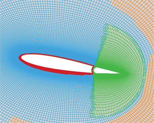
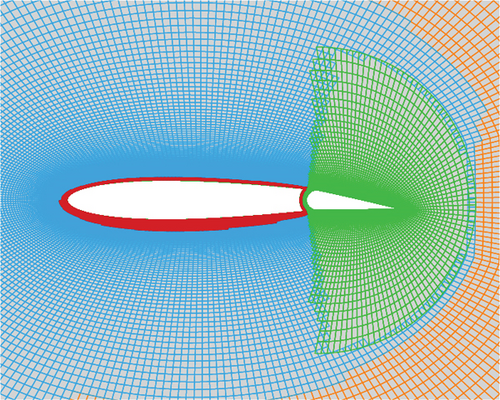
In addition, to enhance computational efficiency, the message passing interface (MPI) parallel strategy is implemented [28]. To this end, the main wing grid is divided into four subzones, each containing an average of 20,000 cells. All the computation cases are performed on a cluster (Intel Xeon Gold 6248R CPU @ 3.00 GHz).
2.2. Governing Equations and Coupling Method
In this study, the lower-upper symmetric Gauss–Seidel [31] method is employed to enhance the solution of the inner iteration step. The inviscid flux is resolved using the Roe [32] flux scheme, while the viscous flux is resolved using the second-order central difference scheme. The incoming Mach number is 0.755, and the Reynolds number, based on the chord length, is 1.76 × 10⁷. Considering the turbulent nature of the flow state, Menter’s k − ω SST [33] turbulence model is implemented.
2.3. Aerodynamic Modeling Methods
Aerodynamic modeling primarily entails establishing the functional relationship between aerodynamic forces or moments and aircraft state parameters. For instance, in the present study, the correlation between the pitching moment coefficient of the airfoil and the angle of attack, as well as the elevator deflection angle would be established. Numerous approaches exist to describe this association, and this paper employs the MNR and ANN methods to accomplish this objective.
The regression method, recognized as a fundamental approach in modeling, has attained widespread application. Initially, the model structure is determined based on aerodynamic characteristics, often relying on polynomials. Subsequently, the coefficients are identified using the least square method. In cases where the dependent variable of the sample might be influenced by several independent variables, a multivariate regression model can be formulated. If a nonlinear relationship is present, a nonlinear regression model can be established. The amalgamation of multiple independent variables and a nonlinear relationship yields an MNR model influencing the dependent variable. When applying the MNR method, it is crucial to initially determine the model structure. For instance, if a polynomial is chosen as the model structure, it is necessary to ascertain the appropriate power of the polynomial. Typically, opting for a lower power may not accurately capture the intrinsic functional relationship of the model, while a higher power can potentially result in overfitting. Thus, it is essential to establish a sensible model structure based on expertise or conducting numerous experiments.
ANN, also commonly referred to as deep learning, has emerged as a prominent focus in the field of ML over the past few years. The application of ANN encompasses two key stages: training and prediction. In the training process, the weights and biases of the network are first initialized randomly. Next, the samples in the training data are predicted using these randomly generated parameters. A loss function is defined to quantify the difference between the predicted values of the network output and the sample values. Essentially, the training process is transformed into an optimization problem in which the goal is to adjust the network parameters to minimize the loss function. The back-propagation algorithm is employed to solve the gradient of all parameters in the model. The gradient information is then used in conjunction with the loss function and the gradient descent algorithm to update the parameters of the ANN model. Ultimately, when the loss function reaches a certain degree of convergence, the training phase comes to an end, and the model can be utilized in the prediction stage. ANN is an effective method for solving problems with nonlinear relationships, even without knowledge of the exact function [34]. Furthermore, the neural network can accommodate any number of input and output variables, and there is no need to predetermine the model structure. Hence, it is highly suitable for modeling complex problems. In this study, ANN is employed to construct the aerodynamic model for the airfoil pitching moment coefficient.
2.4. Control Law Design Methods
This study is aimed at realizing the pitching control of the airfoil. Initially, the deflection angle of the tail is adjusted, resulting in a change in the pitching moment of the airfoil, ultimately causing a variation in the angle of attack. Consequently, two approaches, namely, PID and DRL methods, are selected to accomplish this objective.
DRL is a method that combines deep learning and reinforcement learning. DRL mainly consists of the agent and the environment. The agent interacts with the environment through state, action, and reward [35]. Specifically for this study, the agent is the airfoil, and its state includes parameters such as angle of attack, angular velocity, elevator deflection angle, and the difference between the expected angle of attack and the actual angle of attack. The action is the angular velocity of the tail deflection. The reward function is an indicator that measures the rationality of the selected action in the current state. For example, if the tail deviates at a certain angle, causing the angle of attack of the airfoil to be closer to the expected value, the greater the reward obtained, and vice versa, the smaller the reward. The first step in implementing control using DRL is the training process, where the airfoil selects how to deflect its tail based on the state. Then, tail deflection causes changes in its angle of attack and other state parameters, and the reward function for evaluating this process is returned to the airfoil. By repeating this process, the agent continuously engages in trial-and-error learning based on the reward from the environment and subsequently adjusts and optimizes its state information. Therefore, this is actually a process with feedback, through which intelligent control of airfoil pitch can be achieved. Currently, many efficient algorithms have been developed which has achieved remarkable success in numerous tasks. In this study, the DDPG [36] algorithm is adopted for airfoil pitch control.
3. Verification and Validation
To verify the credibility of the solver, two cases with experimental data are executed. One of them is the flow around a three segments airfoil: 30P30N, used to examine the steady computational ability of the solver; another case is the forced pitching oscillation of the NACA0012 airfoil.
3.1. Steady Flow Around the 30P30N Airfoil
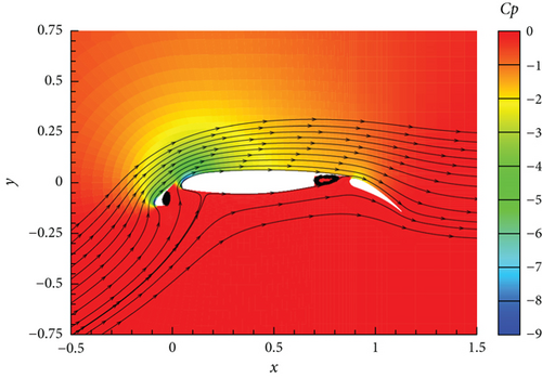
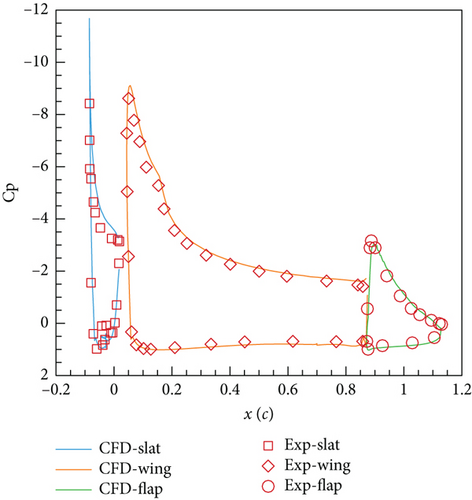
The first case is the flow around a three segments airfoil: 30P30N [37]. This is a steady case study, where each of the three airfoils (i.e., slat, wing, and flap) has its own grid and is combined with the background grid by overset grid method, as shown in Figure 3. This case is mainly used to evaluate the reliability of the solver’s overlapping grids and steady computation. The Mach number of the inflow is 0.2, the Reynolds number based on chord length is 9.0 × 10⁶, and the angle of attack is 16°. Figure 4 shows the contour of the flow field pressure coefficient and streamlines after computation convergence. It can be seen that vortices appear at the lower surface tails of the slat and wing, and at this angle of attack, the suction surface of the wing does not separate. Figure 5 shows the comparison between the computational and experimental data of the surface pressure coefficient, and the two are in good agreement, indicating the reliability of the current solver.

3.2. Unsteady Flow Over the Pitching NACA0012
| Parameter | Value |
|---|---|
| Ma | 0.6 |
| Re | 4.8 × 10⁶ |
| α0 | 4.86° |
| αm | 2.44° |
| k | 0.081 |
Figure 6 displays the computation results of the hysteresis loop of the normal force coefficient for the NACA0012 in pitching oscillation. In steady flow, the angle of attack corresponds one-to-one with the force coefficient; while in unsteady flow, due to the flow change always lagging behind the boundary motion, there is a so-called “hysteresis” effect, so the aerodynamic coefficient angle of attack curve shows a hysteresis loop as shown in Figure 6.
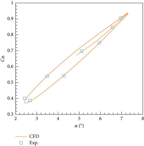
Figure 7 depicts the instantaneous pressure coefficient distribution on the airfoil surface for four phases, and it can be seen that the computed results are basically consistent with the experimental measurements. Note that there are some differences between the CFD results at certain positions of the phase and the experimental data, because it is difficult to ensure complete consistency between the instantaneous angle of attack during the numerical computation process and the experimental instantaneous angle of attack, and there may be some phase errors.
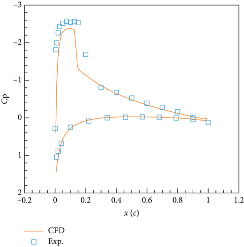

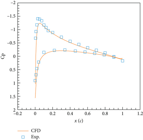
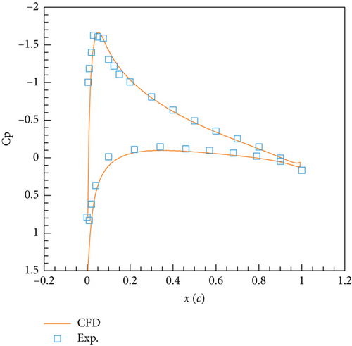
Overall, the current solver computation results reasonably reflect the physical characteristics of the flow in the corresponding state. The hysteresis loop of the normal force coefficient and the distribution of pressure coefficients in each phase obtained from unsteady computation are basically consistent with the experimental values, indicating the reliability of the solver in calculating dynamic aerodynamic characteristics.
4. Results and Discussion
4.1. Grid and Time Step Resolution
4.1.1. Grid Resolution
Grid independence test is related to whether the computation results are trustworthy. For this purpose, five sets of grids are designed by adding the number of circumferential and radial grid points, resulting in a gradual increase in the number of grids. Table 2 lists the number of cells for the main and tail wings with different densities of grids. The number of cells for the main wing are 20,000, 40,000, 80,000, 160,000, and 320,000, respectively. And the number of cells for the tail wing is also gradually increasing, namely, 5000, 10,000, 20,000, 40,000, and 80,000. The comparison of grids with different number of cells is shown in Figure 8.
| Mesh 1 | Mesh 2 | Mesh 3 | Mesh 4 | Mesh 5 | |
|---|---|---|---|---|---|
| Main wing | 20,000 | 40,000 | 80,000 | 160,000 | 320,000 |
| Tail wing | 5000 | 10,000 | 20,000 | 40,000 | 80,000 |
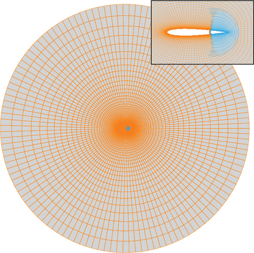
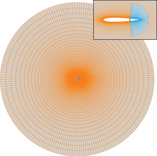
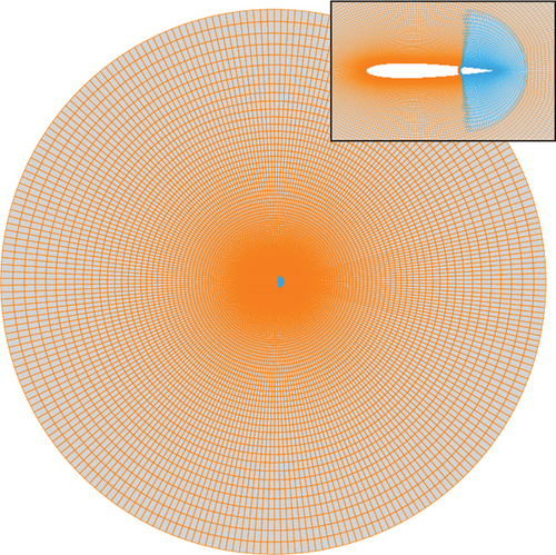
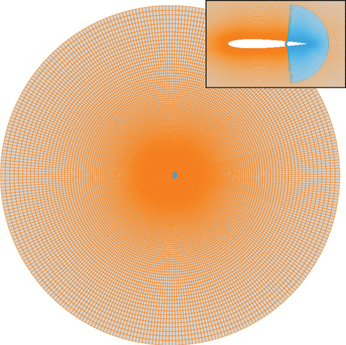

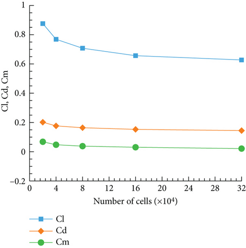
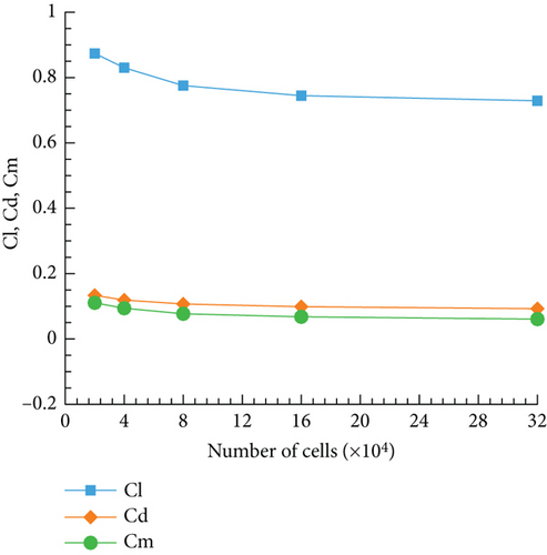
Two cases for these five sets of grids are computed. They are 10° angle of attack and 0° tail deflection angle, as well as 5° angle of attack and 5° tail deflection angle. Figure 9 shows the variation of lift coefficient, drag coefficient, and moment coefficient with grid quantity for these two cases. From Figure 9, it can be seen that as the number of cells increases, the variation of aerodynamic coefficients becomes more gradual. The coefficients change most dramatically during the process of increasing the grid cells from 20,000 to 40,000; The subsequent changes gradually decrease in magnitude. When the grid cells reach 80,000, the changes in aerodynamic coefficients with increasing grid cells are not very significant. Due to the need for a large number of computation cases in this study, considering both computational accuracy and efficiency, it is appropriate to use a grid with 80,000 cells for the main wing and 20,000 cells for the tail wing (Mesh 3).
4.1.2. Time Step Resolution
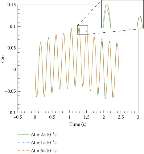
The maximum deflection angle δmax is 5°. For time independence verification, three kinds of time step are taken, namely, 2 × 10⁻³ s, 1 × 10⁻³ s, and 5 × 10⁻⁴ s, to perform unsteady data sampling. Figure 10 depicts the comparison of results among these three. It can be seen that the pitching moment coefficients at three steps have a high degree of overlap. The difference mainly lies in the extreme values, but from the locally enlarged graph, it can be seen that the results with time steps of 1 × 10⁻³ s and 5 × 10⁻⁴ s are also quite close. Therefore, it is reasonable to use a time step of 1 × 10⁻³ s in this study.
4.2. Aerodynamic Data Collection
4.2.1. Steady Computation
The aerodynamic data collected through steady computation involves keeping the main wing and tail stationary while computing the flow field. This process continues until the residual converges, eventually resulting in the aerodynamic moment coefficient. To gather aerodynamic data in this manner, multiple sample points are required across the entire range of angles of attack and elevator deflection angles. For this particular study, the range of angles of attack for the airfoil is set between 0° and 10°, while the elevator deflection angle ranges from −5° to 5°. Thus, we can establish a series of angles of attack ranging from −2° to 12°, with each group consisting of a 2° increment. At each angle of attack, a sample point is set every 2° within the range of −6° to 6°. As a result, this study encompasses 8 groups of angles of attack, with each group having 7 corresponding sets of tail deflection angles. Therefore, a total of 56 cases will be executed in this investigation.
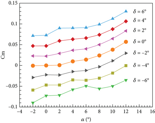
For each case, 5 cores are utilized for parallel computation, and a total of 30,000 steps are executed to attain the converged aerodynamic force. Each case demands 6.28 h of computing on average. Table 3 exhibits the pitching moment coefficients at various angles of attack and elevator deflections; Figure 11 illustrates the variation of the pitching moment coefficient concerning angles of attack for different elevator deflection angles. The depicted information in Figure 11 confirms that as the angle of attack elevates, there is an upward inclination observed in the pitching moment coefficient for different elevator deflection angles. Similarly, keeping the angle of attack constant, a transition from negative to positive elevator deflection angle leads to a gradual rise in the pitching moment coefficient. Moreover, Figure 12 presents a collection of representative pressure coefficient contours under diverse inflow circumstances. The distribution of pressure coefficients in the flow field is notably influenced by distinct angles of attack, while alterations in the deflection angle of the tail wing, at the same angle of attack, can also impact changes in the flow field and consequently affect the moment exerted on the airfoil.
| α | δ = −6° | δ = −4° | δ = −2° | δ = 0° | δ = 2° | δ = 4° | δ = 6° |
|---|---|---|---|---|---|---|---|
| −2° | −0.08982 | −0.05926 | −0.02899 | −0.00062 | 0.02293 | 0.04703 | 0.07153 |
| 0° | −0.07286 | −0.04714 | −0.02245 | −0.00001 | 0.02242 | 0.04709 | 0.07278 |
| 2° | −0.07161 | −0.04709 | −0.02298 | 0.00073 | 0.02892 | 0.05921 | 0.08984 |
| 4° | −0.05808 | −0.03477 | −0.01472 | 0.00985 | 0.03658 | 0.06317 | 0.09023 |
| 6° | −0.04946 | −0.03564 | −0.01199 | 0.01406 | 0.03993 | 0.06598 | 0.09111 |
| 8° | −0.05596 | −0.03060 | −0.00311 | 0.02402 | 0.05005 | 0.07386 | 0.09888 |
| 10° | −0.04982 | −0.01834 | 0.01126 | 0.03804 | 0.06455 | 0.08754 | 0.11257 |
| 12° | −0.03532 | −0.00044 | 0.02957 | 0.05693 | 0.08319 | 0.10629 | 0.13023 |

4.2.2. Unsteady Computation
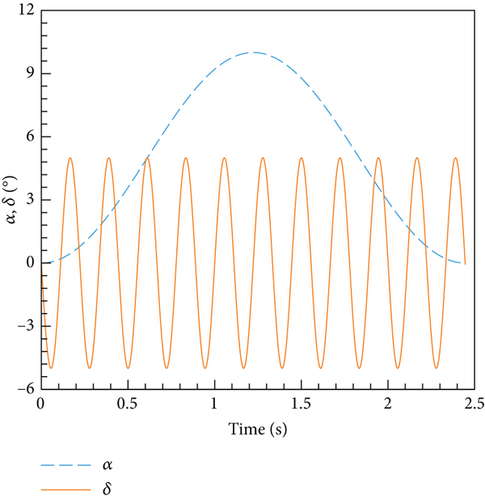
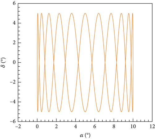
The process of acquiring aerodynamic data through unsteady computation involves first obtaining the initial flow field. Following this, both the main wing and tail wing are individually manipulated to deflect. As the main wing scans through the entire range of angle of attack, the tail wing periodically deflects, ensuring comprehensive coverage of the angle of attack and elevator deflection angle phase space. In this particular study, the angle of attack for the main wing is set to vary according to Equation (12). Additionally, the tail wing is set to deflect periodically according to Equation (13). Consequently, both the angle of attack of the airfoil and the deflection angle of the tail, which serves as the elevator, vary with time according to the depicted pattern in Figure 13. Moreover, Figure 14 illustrates the phase relationship between these two parameters, guaranteeing extensive coverage of the phase space.
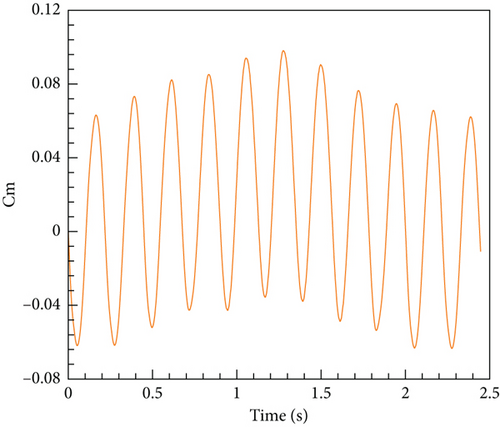
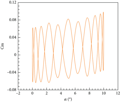
The same computational resources are utilized as in the steady cases, employing 5 cores. Based on the previous time step independence verification, it is appropriate to take an unsteady time step of 1 × 10⁻³ s. The sampling process spanned a total of 2.46 s, consuming 35.72 h of computing resources. The varying pitching moment coefficient with time is visually represented in Figure 15. It is observed that the moment coefficient exhibits periodic fluctuations, which can be attributed to the periodic deflection of the tail wing. The relationship between the moment coefficient and the angle of attack is displayed in Figure 16. As the angle of attack increases, both the maximum and minimum values of the moment coefficient during one cycle of tail wing scanning progressively rise as well. This outcome aligns with the findings obtained from the steady results.
4.3. Aerodynamic Model Construction
4.3.1. MNR Model
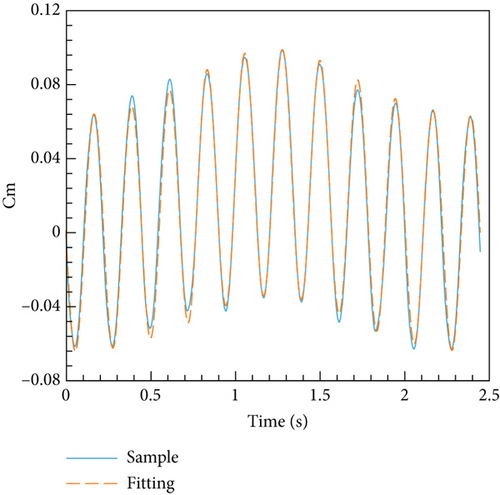
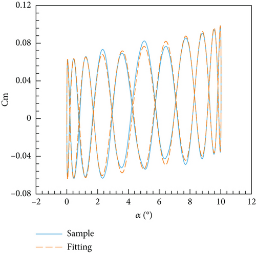
The determination coefficient R2 is 0.9910 and the RMSE is 4.5092 × 10⁻³ of this model, implying a high fit as well. According to this model, the comparison between the original sample data and the fitting data is illustrated in Figure 17, revealing a strong level of agreement. Figure 18 displays the phase relationship between the pitching moment coefficient and the angle of attack. While variations exist in certain regions, the majority of the data demonstrates a remarkable level of consistency.
4.3.2. ANN Model
Similar to MNR modeling, ANN also establishes the correlation between the airfoil pitching moment coefficient and the angle of attack along with the elevator deflection angle. Table 4 lists some parameter settings during the construction of the ANN. In this study, the ANN input layer consists of two neurons representing the angle of attack and the elevator deflection angle. The output layer comprises a single neuron representing the pitching moment coefficient. The hidden layer includes three layers with 32, 64, and 32 neurons, respectively. Each neuron in the hidden and output layers employs the well-known leaky rectified linear unit (ReLU) activation function. The loss function is defined as the mean squared function, while the momentum optimization algorithm is used for network training with a learning rate and momentum factor set to 0.01 and 0.9, respectively. Additionally, the input and output variables are normalized during data preprocessing to enhance learning efficiency and accuracy. The Appendices section compares several different ANN models and confirms the rationality of the current model selection.
| Parameter | Value/function |
|---|---|
| Input dimension | 2 |
| Output dimension | 1 |
| Hidden layers | 3 |
| Number of neurons | 32, 64, 32 |
| Epoch | 10,000 |
| Loss function | Mean squared |
| Activation function | Leaky ReLU |
| Optimizer | Momentum |
| Momentum factor | 0.9 |
| Learning rate | 0.01 |
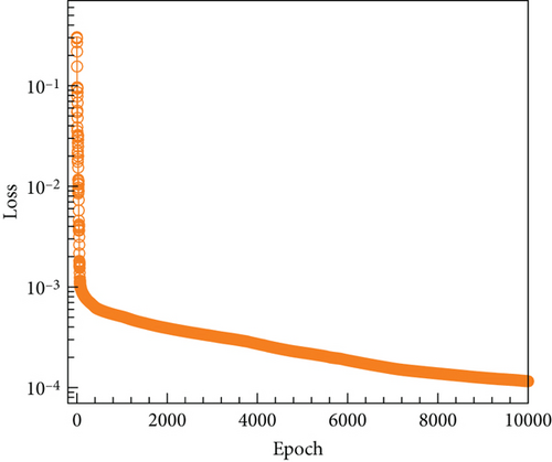
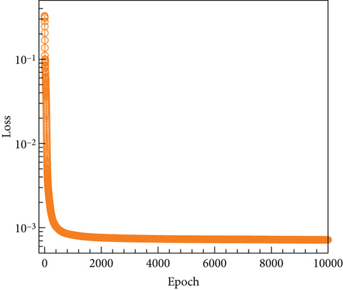
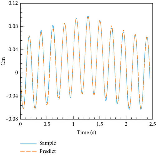
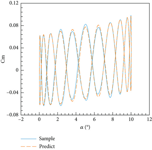
The models established based on steady and unsteady data are called ANN-steady and ANN-unsteady, respectively. The final models are obtained after 10,000 epochs of training. As shown in Figure 19, the loss function quickly converges to a 10−3 level with the number of training epochs increasing. Furthermore, the loss function of the ANN-unsteady model ultimately remained stable; although there are still signs of decline in the loss function of the ANN-steady model, the training is terminated because its loss function value is already small enough. Figure 20 depicts a comparison between the predicted values from the ANN-unsteady model and the original sample data. Remarkably, there is a significant degree of overlap between the two sets. This trend is also evident in the phase diagram of Figure 21, particularly when considering both small and large angles of attack.
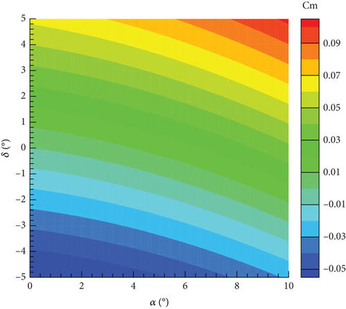
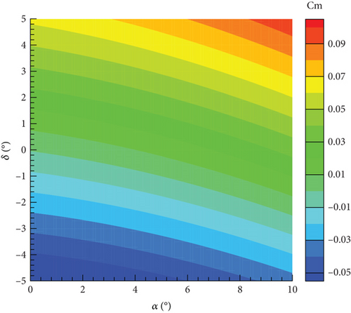
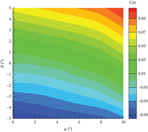
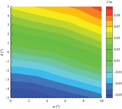
Currently, four models have been established: the MNR model and ANN model based on steady aerodynamic data, and the MNR model and ANN model based on unsteady aerodynamic data. All four models exhibit a high determination coefficient and low RMSE, as shown in Table 5. In addition, it becomes evident that models constructed using the ANN method with the same data possess a superior R2 value and a decreased RMSE in contrast to those developed using the classic MNR method. Moreover, within the same methodology, models established on steady data prove to have a higher R2 value and a lower RMSE when compared to models based on unsteady data. This can be attributed to the limited availability of steady data and a simpler distribution pattern. Figure 22 illustrates the distribution of the pitching moment coefficient obtained from these four models concerning the angle of attack and elevator deflection angle. The distributions of the four models appear to be similar, as the pitching moment coefficient increases with both the angle of attack and elevator deflection angle. However, there are differences between the models as well. The most noticeable distinction is the smooth contour of the MNR model, whereas the ANN model lacks this characteristic. This discrepancy can be attributed to the characteristics of the modeling method. The MNR model utilizes a polynomial structure, resulting in a continuous distribution function. On the other hand, the ANN model lacks an explicit expression and resembles a black box, allowing it to theoretically approximate any function.
| Model | MNR-steady | MNR-unsteady | ANN-steady | ANN-unsteady |
|---|---|---|---|---|
| R2 | 0.9935 | 0.9910 | 0.9981 | 0.9917 |
| RMSE | 4.4196 × 10⁻³ | 4.5092 × 10⁻³ | 2.3672 × 10⁻³ | 4.3313 × −−3 |
4.3.3. Model Verification
Here, two cases are designed, with the first case δmax = 1° and T = 1 s, representing weak unsteady flow. The second case, δmax = 5° and T = 0.25 s, represents a strong unsteady effect. Figures 23 and 24 illustrate the variations in elevator deflection angle, pitching moment coefficient, angular velocity, and angle of attack over time for the two cases, respectively. The deflection of the tail wing causes the moment acting on the airfoil to become unbalanced. As a result, the airfoil experiences acceleration under the influence of this, thereby generating angular velocity and ultimately altering the angle of attack.
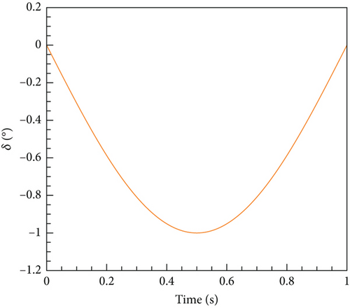
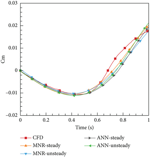
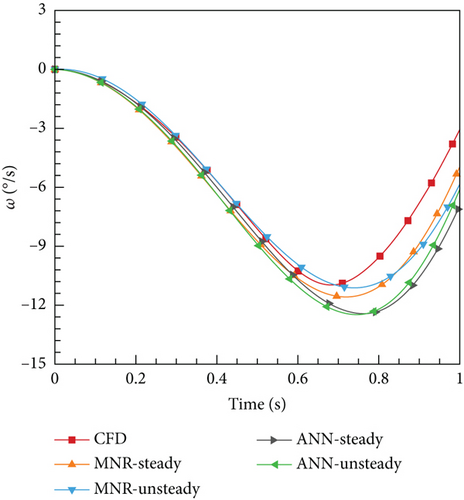
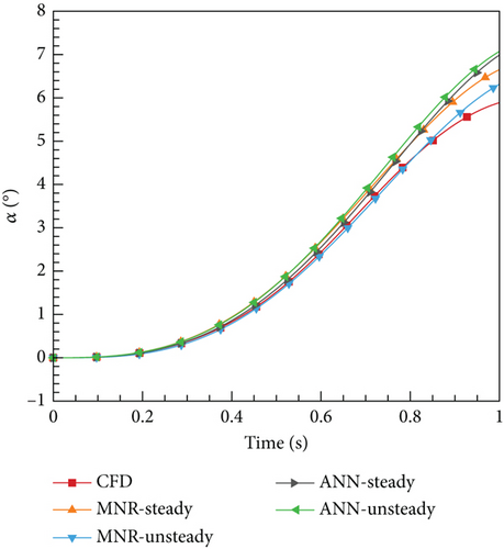
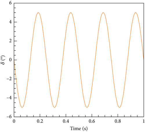
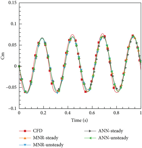
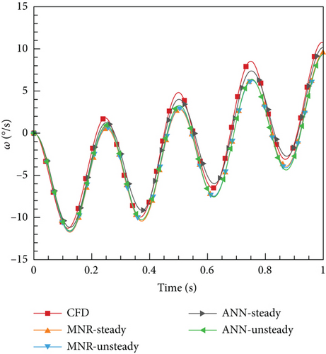

From Figures 23 and 24, it is evident that all four aerodynamic models produce computation results consistent with the trends observed in CFD. However, there are some differences between the cases as well. In Case 1, four models yield more consistent results with CFD compared to Case 2. This can be attributed to the weak unsteady characteristics of the current case, where all models can reflect the dynamic characteristics adequately. For Case 2, due to the enhanced unsteady effects, the MNR-steady model, relying on steady data, performs comparatively worse than the two other models based on unsteady data. However, it is surprising that the ANN-steady model demonstrated the highest level of consistency with the CFD results. The change in the angle of attack curve for this model is closely aligned with the CFD results. On the contrary, the MNR-steady model, which also utilized steady data modeling, performed poorly compared to the other models in this specific case. Hence, it can be concluded that the modeling method played a crucial role in this process. What could be the underlying reason for this phenomenon? As mentioned earlier, the ANN possesses the remarkable ability of universal approximation and naturally exhibits properties that are ideal for processing data. Furthermore, it does not depend on the specific function structure, allowing it to have a strong generalization ability. This ability often leads to unforeseen effects in certain outcomes, which could explain why deep learning has become almost synonymous with ML today. However, to uncover a more fundamental reason, researchers would still need to conduct extensive exploration.
Based on the aforementioned results, it is more reasonable to select a data collection method according to the unique characteristics of the movement itself. However, the actual scenario presents an aircraft with both weak unsteady flow and strong unsteady effects, necessitating a comprehensive consideration of these factors. Furthermore, it should be noted that steady computation requires substantial computational resources and time. In this study, the time required for steady data collection is as much as 10 times greater than that for unsteady data sampling. Therefore, employing an unsteady computational data sampling method proves to be a more efficient approach. Concerning modeling, it is evident that the ANN method outperforms the MNR method in terms of determination coefficient and RMSE for the same set of data. Unlike the MNR method, the ANN method does not require determining a model structure to display a formula. Instead, it operates without explicit formulas, which liberates it from reliance on prior experiences and grants it superior generalization ability, leading to unforeseen outcomes. Although this study solely concentrates on relatively simple situations, the aviation industry frequently encounters more intricate scenarios, thus indicating that the ANN method is likely to hold even more advantages in such contexts.
4.4. Control Law Design
4.4.1. PID Control
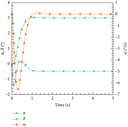
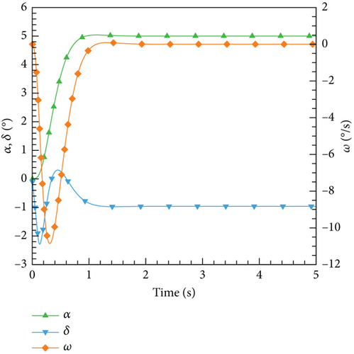
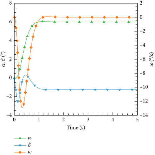
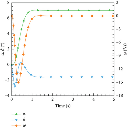
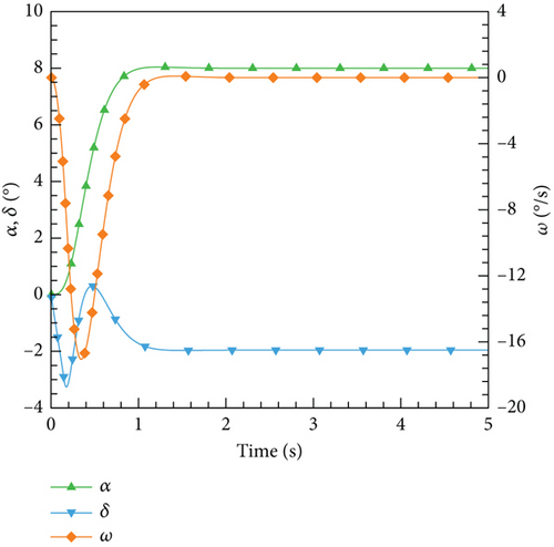
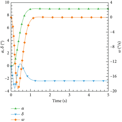
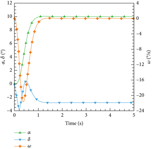
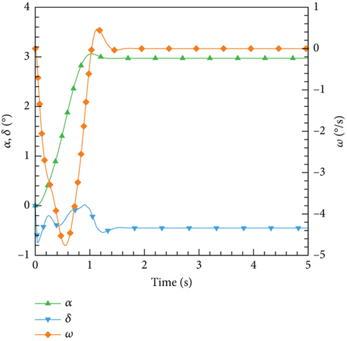
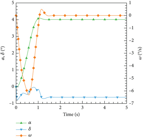
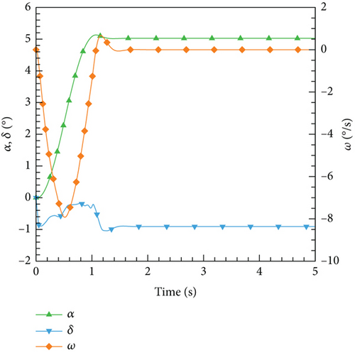
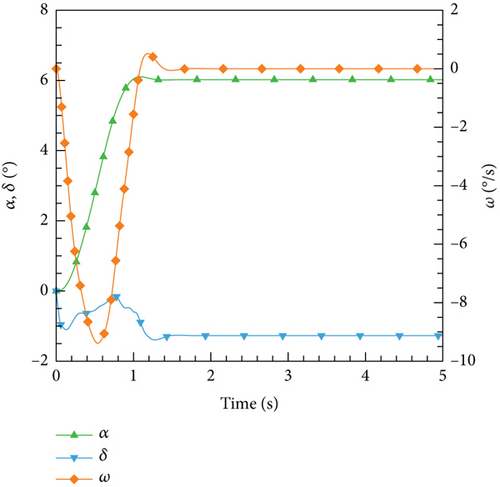
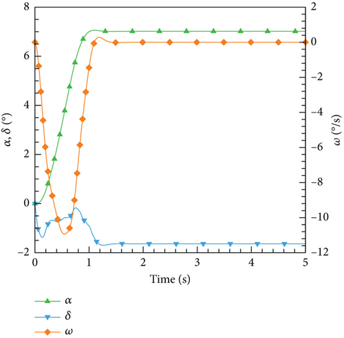
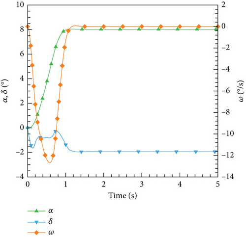
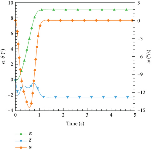
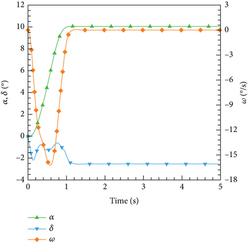
Although there exist relevant theories and methodologies to determine the coefficients of Kp, Ki, and Kd, the trial-and-error approach is still employed to ascertain them based on the MNR-steady model in this study. The principle throughout this process is to achieve the expected angle of attack in approximately 1 s while minimizing both steady-state errors and oscillations as much as possible. During the control procedure, the parameters are sampled and updated every 0.005 s, and the maximum deflection rate of the elevator is limited to 20°/s. The final coefficients obtained are Kp = 50, Ki = 0.725, and Kd = 1500.
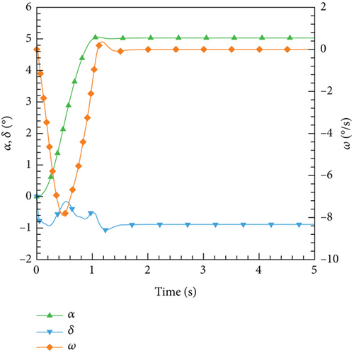
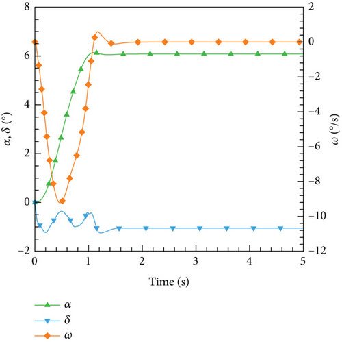
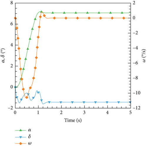
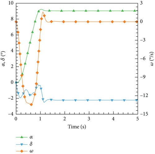
According to this control law, the control results for various expected angles of attack are illustrated. In Figure 25, the variations of the angle of attack, elevator deflection angle, and airfoil pitch angular velocity with time are depicted. It can be observed that PID as a classic control algorithm can effectively meet different control needs and maintain stability throughout the entire process.

4.4.2. DRL Control
| State | Normalization | Description |
|---|---|---|
| α | α/αmax | The maximum angle of attack is about 10°, normalized to [0, 1]. |
| ω | ω/(0.5ωkαmax) | The maximum angular velocity is about 0.5ωkαmax, normalized to [−1, 1]. |
| δ | δ/δmax | The maximum deflection of the elevator is 5°, normalized to [−1, 1]. |
| Δα | Δα | The maximum allowable deviation from the αref is 1°, normalized to [−1, 1]. |
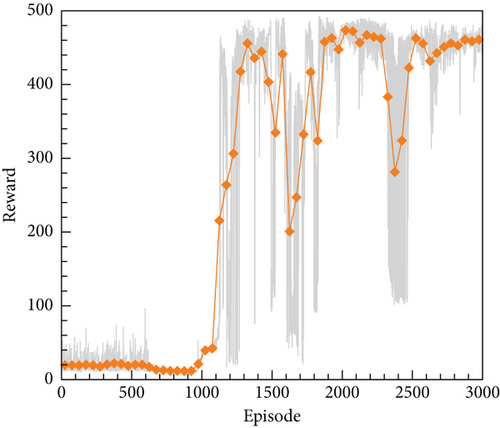
The actor and critic networks of the DDPG algorithm consist of single hidden layer neural networks, and the activation function utilized is the leaky ReLU. Prior to the commencement of each episode, αexp is randomly chosen, ensuring that the difference between the angle of attack and the reference angle of attack remains within 1°. If this difference exceeds the specified limit, the training episode will be terminated. Each episode is allowed a maximum of 500 steps, and a total of 3000 episodes of training are conducted. The other related parameter settings for the DDPG algorithm are shown in Table 7. The variation of the reward function with the number of training episodes is shown in Figure 26. The orange line with diamond markings represents the moving average reward function, which is the average reward for every 50 episodes. During the initial stage, the agent primarily focuses on trial and error, thus possessing a high level of exploration and consequently obtaining relatively low reward values. As the exploration reaches a certain threshold, the agent shifts its focus towards utilizing the experience gained in the early stages for action selection. Consequently, during this phase, the level of exploration is maintained at a low level and reward remains at a high level.
| Parameter | Value |
|---|---|
| Episodes | 3000 |
| Episode steps | 500 |
| Actor learning rate | 3 × 10⁻⁴ |
| Critic learning rate | 6 × 10⁻⁴ |
| Reward discount | 0.95 |
| Memory capacity | 2 × 10⁴ |
| Batch size | 64 |
After the training session, the DRL control law derived is then implemented and evaluated on the ANN-unsteady model, with the performance results depicted in Figure 27. It is worth noting that the agent accomplished the assigned tasks with exceptional accuracy, regardless of the varying angles of attack.
4.4.3. Integrate the Control Laws Into the CFD-Based NVF Environment
Currently, two types of control laws have been successfully developed and performed effectively on their respective aerodynamic models. These control laws are now utilized in a CFD-based NVF environment to assess their generalization capability and effectiveness in aerodynamic systems.
Figure 28 depicts the application of the PID controller in the CFD-based NVF environment and demonstrates its high accuracy and efficiency performance. Additionally, Figure 29 illustrates the Mach contour for each case after it reaches a stable state. As the angle of attack augments, the upper surface exhibits a gradual migration of the high Mach number region towards the airfoil’s leading edge. Correspondingly, the low Mach number region at the tail progressively extends forward. Consequently, the airfoil’s pitching moment amplifies, necessitating an increase in the deflection angle of the tail during equilibrium.
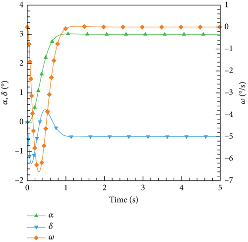
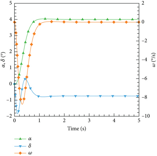
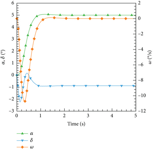
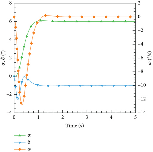
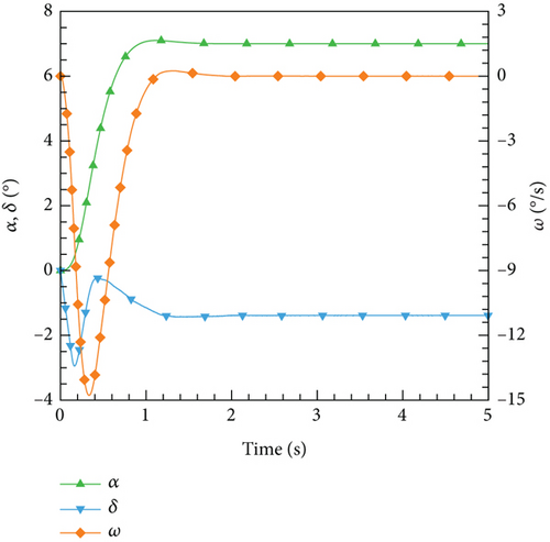

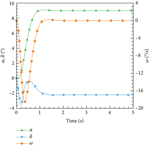

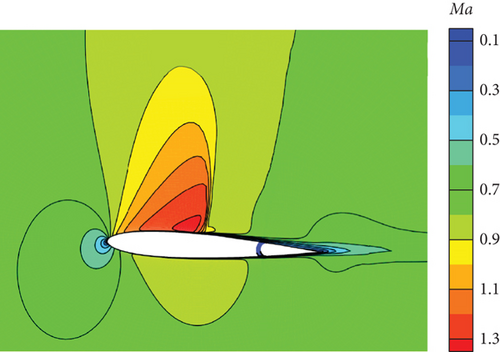
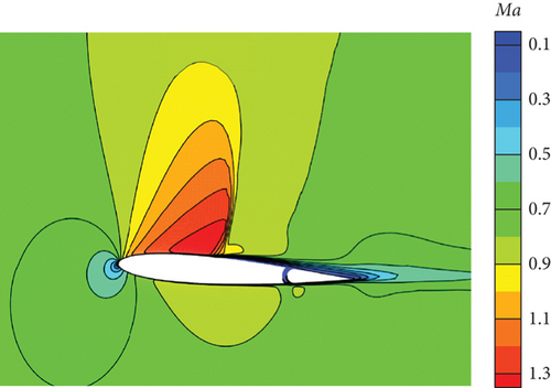
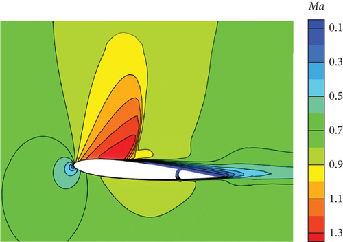
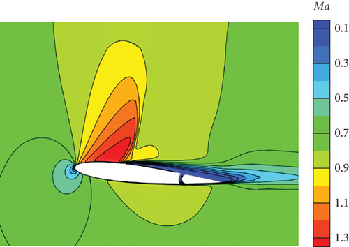
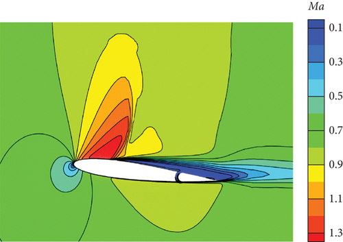
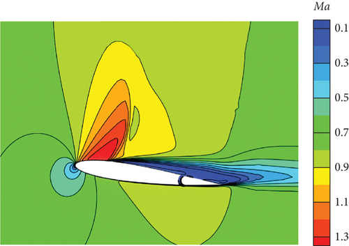
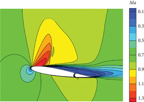
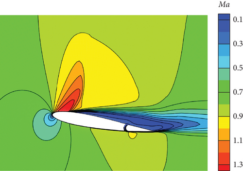
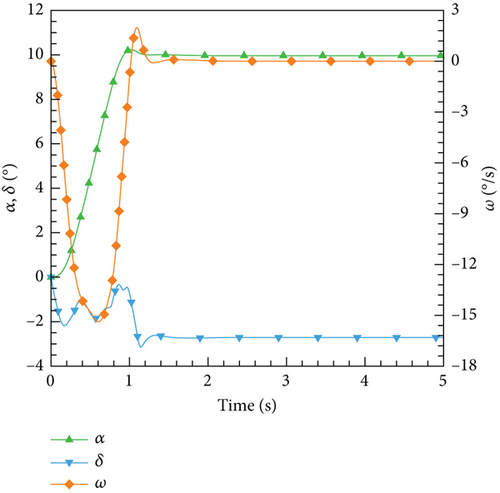
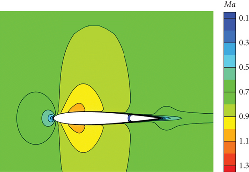
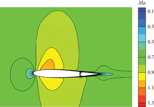
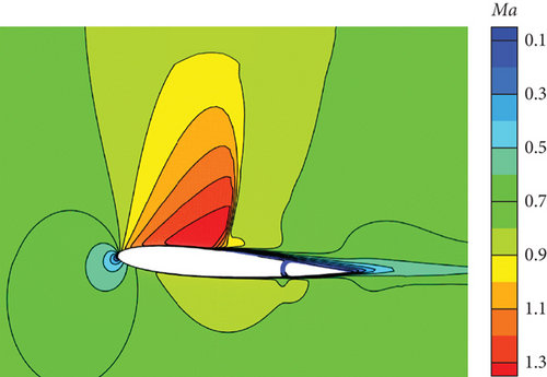
Figure 30 illustrates the outcomes achieved through the implementation of the DRL controller in the CFD-based NVF environment. In line with the performance exhibited by the ANN-unsteady model, the agent effectively accomplishes the task across various expected angles of attack. In Figure 31, the Mach contour is depicted at different time intervals for the scenario where αexp = 10°. Initially, the flow field on both the upper and lower surfaces of the airfoil is symmetrical (Figure 31(a)). However, as the elevator starts to deflect, the angle of attack gradually escalates. Consequently, the flow field experiences alterations on both the upper and lower surfaces of the airfoil, resulting in an imbalance of forces and subsequent pitch of the airfoil (Figures 31(b), 31(c), and 31(d)). Through the manipulation of the elevator, the airfoil progressively adjusts itself to reach the expected angle of attack and eventually maintains this angle (Figures 31(e) and 31(f)).
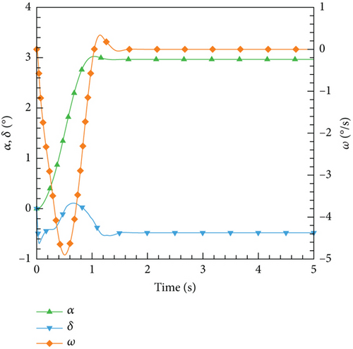
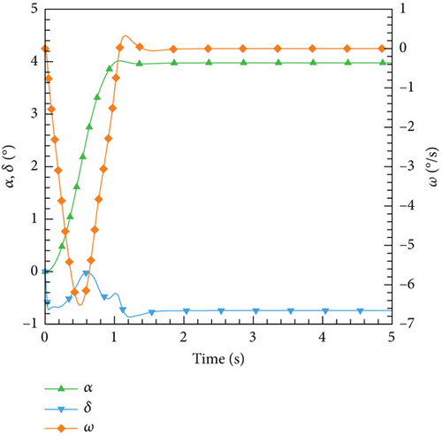

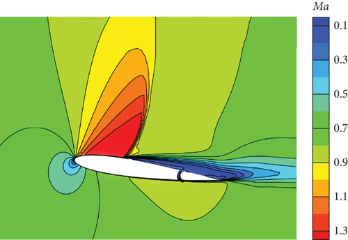
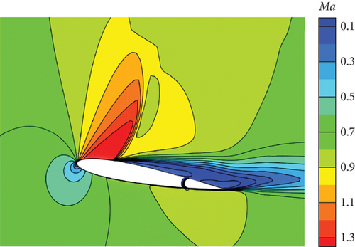

However, based on the current findings, it is challenging to determine the superiority or inferiority of different control methods. The primary reason for this is that the research focuses solely on the linear domain of airfoil pitch control, which is precisely the advantage area of the classical PID control method. Nonetheless, these cases demonstrate the potential for implementing AI techniques in the aviation industry. In more intricate flight settings, demanding missions, and diverse application scenarios, it becomes imperative to explore the effective integration of AI. This exploration will ensure enhanced safety and efficiency in flight control and propel the aviation industry into the era of intelligence.
5. Conclusion
This study focuses on a modified NACA0012 airfoil and is aimed at achieving a comprehensive set of processes through numerical simulation. These processes include data sampling, aerodynamic modeling, control law design, and transferring the control laws to the CFD-based NVF environment. Classical methods as well as ML techniques are employed throughout the research process. To begin with, aerodynamic data sampling is essential. To obtain multiple data points, a significant number of cases need to be set up for steady computation. This, however, consumes a substantial amount of computing resources. On the other hand, unsteady data sampling allows for the collection of aerodynamic data by scanning the entire parameter space, ultimately saving computational time. Moving on to aerodynamic modeling, limited aerodynamic data generated by the steady method could use the MNR and ANN methods to establish effective models. In contrast, unsteady computation sampling generates a vast amount of aerodynamic data, and ANN exhibits natural advantages over the MNR method in establishing a more accurate model. Moreover, the model established with ANN can show surprisingly perfect results. Lastly, the study delves into the control law design method. While the classic PID control method excels in handling single objective and linear control, the DRL method presents a new approach that holds promise for broader application in the aviation field. In future work, these methods will be applied to the study of three-dimensional engineering-shaped air vehicles, such as missiles and aircraft.
Conflicts of Interest
The authors declare no conflicts of interest.
Funding
This work is supported by the National Key Project (grant number GJXM92579); the Scientific Research Innovation Project of Graduate Student of Hunan Province (grant number CX20230017); and the National Science Foundation of China (grant number 92252101).
Acknowledgments
This work is supported by the National Key Project (grant number GJXM92579); the Scientific Research Innovation Project of Graduate Student of Hunan Province (grant number CX20230017); and the National Science Foundation of China (grant number 92252101).
Appendix
The ANN model chosen currently does not have a clear theoretical guidance and more often relies on the experience and attempts of the researcher. Too few and too many network layers and neurons are both inappropriate. Too few may lead to underfitting and insufficient model accuracy, while too many can increase computational complexity and overfitting. In this study, the common symmetrical structure with an increase firstly and then a decrease in the number of neurons is selected, and the hidden layer is determined to be 3 layers. To justify this choice, the number of layers as well as the activation function are changed, and then they are trained on the different datasets for comparison. Table A1 shows detailed information on different networks.
| Hidden layers | Number of neurons per layer | Activation function | |
|---|---|---|---|
| Network 1 | 1 | 64 | Leaky ReLU |
| Network 2 | 3 | 32-64-32 | Leaky ReLU |
| Network 3 | 5 | 16-32-64-32-16 | Leaky ReLU |
| Network 4 | 3 | 32-64-32 | Tanh |
Figure A1 illustrates the decline in loss function for different networks when trained on the steady dataset. It can be seen that there is a significant difference in the loss function between Network 4 and the other three networks: It still has a relatively high value after training. For the other three networks, at the end of training, the difference between Network 2 and Network 3 is smaller than the difference between Network 1 and Network 2. Therefore, it is necessary to increase the number of layers and neurons in the network from Network 1 to Network 2, while increasing from Network 2 to Network 3 is not as effective as before. Figure A2 shows the performance of these networks on the unsteady dataset. There is a significant difference between Network 4 and the other three again, while the difference between Networks 1, 2, and 3 is very small.

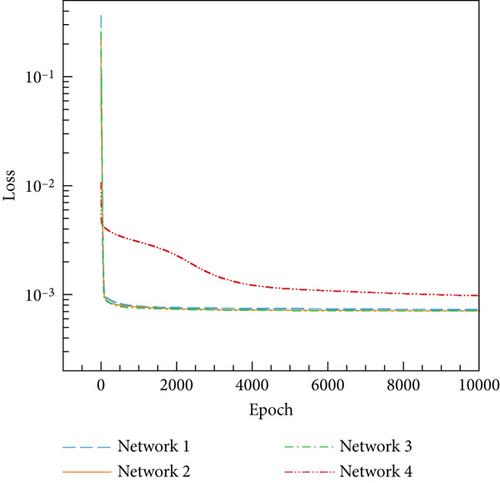
Meanwhile, the determination coefficient and the RMSE of different networks are also statistics, as shown in Table A2. Based on the determination coefficient and the RMSE, the above conclusions can also be drawn that there is a significant difference between Network 4 and the other three networks. As the number of network layers and neurons increases, the performance improvement of the other three networks is significant on the steady dataset, while they are exceptionally close on the unsteady dataset. Therefore, considering various factors comprehensively, the selection of Network 2 in this study is reasonable.
| Steady dataset | Unsteady dataset | |||
|---|---|---|---|---|
| R2 | RMSE | R2 | RMSE | |
| Network 1 | 0.9966 | 3.1889 × 10⁻³ | 0.9916 | 4.3730 × 10⁻³ |
| Network 2 | 0.9981 | 2.3672 × 10⁻³ | 0.9917 | 4.3313 × 10⁻³ |
| Network 3 | 0.9984 | 2.2002 × 10⁻³ | 0.9919 | 4.2952 × 10⁻³ |
| Network 4 | 0.9866 | 6.3435 × 10⁻³ | 0.9887 | 5.0616 × 10⁻³ |
However, it must be acknowledged that this is only a simple analysis. Due to the multitude of elements in neural networks, a large number of ANN models can be yielded by changing these variables. Therefore, only a simple comparison is made regarding the number of layers and neurons in the network structure, as well as the activation function. The best model may be obtained through extensive numerical experiments, but for this study, the use of a simple network is sufficient to meet the requirements.
Open Research
Data Availability Statement
The data used to support the findings of this study are included within the article.


