1. Introduction

Bridges are essential infrastructures that significantly impact social and economic development [1, 2]. However, bridges inevitably experience damage and degradation due to environmental and accidental factors [3, 4]. This affects the load-bearing capacity and operating conditions of bridges. Thus, detecting minor damage to bridges at an early stage and conducting repairs and rehabilitation can effectively prevent the loss of life and economic damage caused by failures [5, 6]. In addition to the practical requirements of bridges and other structural inspections, many methods for structural damage identification have been studied. They can be categorized as model-based and model-free damage detection methods [7–9].

Model-based damage identification methods require an accurate numerical model of the target structure that infers unknown parameters from structural measurements [10–12]. Many damage identification studies have relied on structural models. Zhang and Xu [13] investigated a multilevel damage identification method based on response reconstruction. Damage detection was performed at the macroelement level, followed by further identification of substructures to locate and quantify the damage. Figueiredo et al. [14] developed a model-based finite element machine learning approach to detect damage. Simulated and test data were combined, which could reduce false positives caused by environmental variations and improve the accuracy of bridge detection. Zhang and Sun [15] investigated a damage identification approach using physics-guided machine learning that combines pattern recognition with finite element model updating. Numerical and experimental validation showed that the method can improve the accuracy and versatility of damage detection. Hassani et al. [16] proposed a damage-sensitive feature that is sufficient for handling nonstationary brown noise. This sensitive feature developed a novel and robust method for model updating of structures with closely spaced eigenvalues. Malekghaini et al. [17] proposed a time-domain Bayesian finite element model updating technique. Vibration data and measured dynamic responses at the locations of vehicles crossing the bridge were used to estimate the vehicle loads and finite element modeling parameters for the bridge. Li et al. [18] proposed a damage detection method based on a domain-adversarial neural network, where the displacement responses of a finite element model and an actual bridge under moving loads were used as inputs for adversarial training and the extraction of common damage features. Wang et al. [19] proposed a damage indicator for steel truss bridges based on a statistical steady-state strain characteristic function, and a digital twin model for damage identification and a framework for in-service damage identification systems were established. The primary advantage of the model-based approach is its ability to facilitate physical interpretation of the detected damage. However, the construction of precise and comprehensive finite element models presents significant challenges. In addition, the presence of numerous unknown parameters substantially complicates the associated inverse and optimization processes.

Model-free damage detection does not require the establishment and updating of numerical models. Most model-free methods utilize artificial intelligence techniques to train classification algorithms on the data of a structure and rely on the data to reveal the relationship between healthy and damaged structures. Although model-free methods cannot yield a physical explanation for damage, they are computationally convenient [20–22]. Li and Wu [20] proposed a model-free method for damage localization and quantification based on the correlation of modal parameters among distributed fiber-optic sensors. A polynomial equation representing the relationship between the damage index and the degree of damage was used for damage quantification. Moreover, Suwała and Jankowsk [23] proposed a model-free method for identifying changes in structural mass based on the virtual distortion method. This method does not require a parametric numerical model of the monitored structure or any topological information. Furthermore, Xu et al. [24] proposed a damage identification method based on the principal, mean, and Gaussian curvature mode shapes. The method is non-model-based and does not require any a priori information on the relevant undamaged plates. In addition, Chen et al. [25] proposed a multiple damage identification method for nonmodeled beams based on a continuous scanning laser Doppler vibrometer system. This method utilizes the curvature of the operating deflection shapes with the curvature damage indices of a polynomial fit to the difference to identify multiple damages. Ma et al. [26] introduced a data-driven approach based on sensor network data that exploited spatiotemporal correlation for accurate sensor data reconstruction. Gaussian process regression was used to learn the spatiotemporal behavior of the system, and the uncertainty was quantified using Bayesian posterior probability outputs. Xu et al. [27] proposed a damage identification method for large-span spatial structures based on a time-series analysis of acceleration data. Autoregressive parameters and Mahalanobis distance were used to discriminate damage-sensitive features constructed by the discriminant function. The effectiveness of the proposed method was verified using numerical modeling. Sarmadi et al. [4] proposed a probabilistic data self-clustering method based on semiparametric extreme value theory (SEVT) and peak-over-threshold (POT) for anomaly detection and threshold estimation. The problem of damage under severe environmental variability was addressed.

The behavior of large structures is often complex, and the construction of accurate models is redundant and complicated. Moreover, inaccurate computational models may lead to unreliable feature identification [28–30]. Simultaneously, damage identification for large structures is time-consuming. Model-free methods require a large amount of characterization data for both healthy and damaged conditions. Therefore, an important challenge in the application of model-free methods is the lack of damage characterization data [31, 32]. In this study, a partial model-based damage identification method is proposed for the damage identification of long-span steel truss bridges, and this method extends the stiffness separation method of the previous study [33–35]. The innovation of this study is to employ partial model information to identify the damage and circumvent the establishment of the overall structure stiffness equation, simplifying the modeling complexity. This method improves the feasibility of the damage identification based on the partial model information. Moreover, the quantification of member damage through a partial model of the structure can reduce the accumulation of modeling errors to a certain extent. The remainder of this paper is organized as follows: Section 2 introduces the theory of the identification method. Section 3 discusses the analysis of a long-span steel truss bridge and parameter estimation using two optimization algorithms. The paper concludes with a summary in Section 4.

2. Damage Identification Method Introduction

Structural parameter estimation, a powerful tool for updating analytical models based on structural responses, is widely used in structural health monitoring. Parameter estimation methods analyze the extent of structural damage by comparing the error of the estimated response with the actual condition [36, 37]. This section reviews general parameter estimation methods for static-based space truss structures. A partial-model-based parameter estimation method was presented.

2.1. General Static Parametric Estimation Method

The space truss element is illustrated in Figure 1. Assuming that the cross-sectional area of the element is A, the modulus of elasticity is E, and the length is L. Subsequently, the global stiffness matrix of the element can be expressed as follows:

$$ ()

where λ_x = cos θ_x,  λ_y = cos θ_y,  λ_z = cos θ_z, and θ_x,  θ_y,  θ_z denote the angles of the member measured from the global x, y, and z axes, respectively, to the local x^′ axis. Herein, x^′ is directed along the element from node 1 to node 2.

The truss structure consists of numerous elements. The stiffness matrix of the overall structure can be obtained from the elemental stiffness matrices of all members by algebraic summation. The structure stiffness equation of the overall structure is as follows:

$$ ()

where K denotes the stiffness matrix of the overall structure and D and Q denote the displacements and external loads of the structure, respectively. The DOFs with unknown displacements in the structure are set to the lowest code numbers, and the equation can be divided as follows:

$$ ()

where Q_k and Q_u are the known and unknown forces, respectively, and D_k and D_u are the known and unknown nodal displacements, respectively.

When damage occurs in a structure, the structural stiffness decreases. Representing the damage caused by a decrease in the area of members is a commonly used method for structural damage identification. Assuming that the cross-sectional area of the member after damage is A_d, all the area data after damage are included in the vector A_d. In this study, the areas of the members after damage were unknown and needed to be determined. Therefore, the structure stiffness matrix K in the structure matrix stiffness equation contains the parameter A_d; thus, the solved nodal displacements contain unknown parameters, as follows:

$$ ()

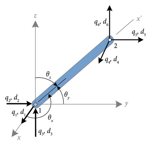
Based on the nodal displacements at both ends and the stiffness matrix of the truss element, the analytical strain of the element can be easily obtained. The objective function is then established by combining the measured element strains. To minimize the difference between the analytical and measured strains, an optimization method is used to determine the minimum value of the objective function, and the optimal parameters can be identified.

2.2. Partial-Model-Based Parametric Estimation Method

If the structure is large, then the dimensions of the structure stiffness matrix are also large. Therefore, the inversion calculation is difficult. A stiffness separation method was proposed to simplify the large-structure inversion problem [33, 34]. The stiffness separation method establishes the equilibrium equation by separating the relevant parts of the substructure from the overall structural force-displacement equations. The unknown displacements of the substructure are then solved. The equilibrium equation of the substructure is given as

$$ ()

where K^′ is the partitioned matrix of the substructure with dimensions m × n, D^′ denotes the combination of the known and unknown displacements of the substructure with dimension n, and Q^′ denotes the known load of the substructure with dimension m. The aggregate of the substructure DOFs is n, and the substructure’s number of unknown displacements DOFs is m. This paper proposes a damage identification method that utilizes the stiffness of a partial model. This method is intended to solve cases wherein partial information concerning the overall structure is missing or the structure is complex and assembling the stiffness matrix of the overall structure is time-consuming. The damage identification method assembles only partial model information and avoids assembling the overall stiffness matrix.

It can be observed in the truss element shown in Figure 1. If the spatial location of an element is known, the stiffness equation of the element e can be expressed through the following equation:

$$ ()

Herein, the stiffness matrix of the element is denoted as k^e. Each term of k^e, $$, represents the force component required in the direction of i DOF when the eth element undergoes a unit displacement in the direction of j DOF. In equation (6), q₁, q₂, q₃ and d₁, d₂, d₃ represent the forces and displacements in the x, y, and z directions at the near end of the member. q₄, q₅, q₆ and d₄, d₅, d₆ represent the forces and displacements in the x, y, and z directions, respectively, at the far end of the member. Once the damage region to be identified has been determined, the matrix K^′ of the partial model can be assembled using some or all the stiffness influence coefficients for each element in the region. Solving the partial model equilibrium equation allows for the determination of unknown displacements. Thus, the calculation of the stiffness matrix for the overall structure can be avoided. The partial model’s matrix K^′ can be obtained using the following equation:

$$ ()

Note that $$ denotes the algebraic addition of stiffness influence coefficients for the corresponding members in the partial model, where i ranges from 1 to m and represents the DOFs of the unknown displacements in the partial model. j ranges from 1 to n and represents the DOFs of the partial model. N represents the number of members in the partial model. Therefore, the stiffness influence coefficients out of the partial model equations can be disregarded.

The partial model displacements can be categorized into unknown displacements $$ and known displacements $$ as follows:

$$ ()

where the size of $$ is m, and the size of $$ is (n − m). Matrix K^′ is then divided according to the DOFs of the displacements as follows:

$$ ()

where $$ is a square matrix of order m and contains the stiffness influence coefficient k_ij (i,  j ∈ (1, …, m)). $$ is an m × (n − m) matrix and assembled from the stiffness influence coefficients k_ij (i ∈ (1, …, m);  j ∈ (m + 1, …, n)). Taking equations (8) and (9) into equation (5) yields

$$ ()

The damaged condition was set as variable A_d. Subsequently, for the partial model, the stiffness contained a variable A_d, and the unknown displacements were obtained using the following equation:

$$ ()

Subsequently, the analytical strain ε(A_d) can be determined by the strain-displacement relationship. The objective function is the sum of the squares of the differences between the measured strain ε^′ and analytical strain ε(A_d)

$$ ()

In equation (12), M denotes the total number of measured strains. Parameter estimates can be obtained by minimizing the function value of f(A_d). $$ denotes the vector set of optimized values

$$ ()

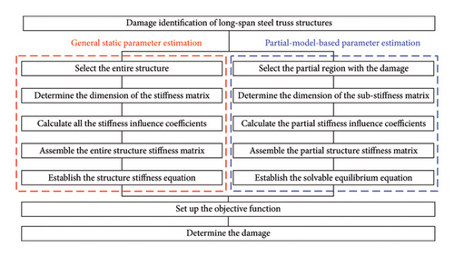
Overall, performing structural damage identification using the general static parameter estimation, the entire structure stiffness equation is required to be established. Therefore, all the member stiffness matrices of the entire structure need to be determined and their stiffness influence coefficients need to be assembled in the overall structure stiffness matrix. However, the size of the stiffness matrix is large as the DOFs increase. The process of assembly of the structure stiffness matrix is complicated. Instead, the partial-model-based parameter estimation is to assemble the matrices related to the DOFs in the partial model, and only the corresponding stiffness influence coefficients need to be calculated and assembled. The size of the matrix is therefore reduced, and the assembly efficiency is significantly improved. Figure 2 illustrates the flowchart of the damage identification. The red and blue boxes represent the process of general static parameter estimation and the partial-model-based parameter estimation.

3. Illustrative Case Studies

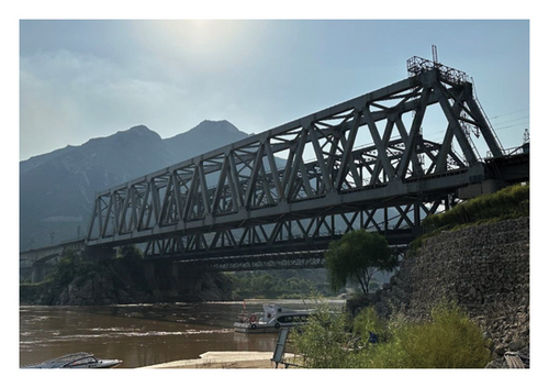
In this section, a long-span bridge in service is used to illustrate the feasibility of the proposed damage identification method. The New Yellow River Bridge was built in 2015, and this bridge crosses over the Yellow River, which is the second longest river in China. The New Yellow River Bridge is a simply supported steel truss railroad bridge connecting the central of Shaanxi Province and south of Shanxi Province, and this bridge is located near Yumenkou station of the Huang-Han-Hou railway line. It is a long-span bridge with a span length of 156 m, 11 panels, a height of 17 m, and a width of 8.6 m. According to data from 2017 [38], this bridge is the longest simply supported steel truss railroad bridge in China, as shown in Figure 3. In this study, the secondary components of the bridge were simplified, and parts such as portal and sway bracings were omitted. In addition, the tracks and bridge deck were not included, and all the nodes were pin-connected joints. Pin supports were installed at nodes 1 and 2, and rocker supports were installed at nodes 45 and 46. Figure 4 shows the simplified structure. The red numbers in the figure indicate the numbering of members, and the blue numbers indicate the labeling of nodes. Simultaneously, displacement constraints were applied in the Y direction at nodes 3 and 4, as well as nodes 43 and 44, to ensure stabilization of the structure. In the structure, the structural steel’s modulus of elasticity is 210 GPa. The cross-sectional area of the upper lateral bracing is 18,216 mm². The area of the top lateral strut is 17,576 mm². The lower lateral bracing area is 22,272 mm². The cross-sectional areas of the remaining members are listed in Table 1. Moreover, considering the symmetry of the structure, the “as-built” cross-sectional areas of the members of the truss are shown only for the members located in the plane of nodes 1, 3, 43, and 45. The areas of the members on opposite sides correspond to the same area.

3.1. Left Region Damage Identification

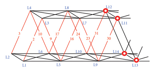
Assuming that the damage was concentrated and distributed in the left region of the structure, vertical loads of 100 kN were applied at nodes 9 and 10 locations to make the structural response more pronounced in this region. The structure was isolated using displacement sensors, as shown in Figure 5(a), where the circles on nodes 11–14 represent the positions of the displacement sensors. The partial model used for the analysis is shown in Figure 5(b). For the analysis, it is assumed that the damaged members are located in the diagonal members and end posts, and the “as-is” areas of the members after damage are shown in Table 2 for a total of 10 members. Damage identification was performed on the members of the truss (shown in red), and strain sensors were located on these members. In this study, the measured displacement and strain were determined based on the artificially induced damage scenarios.

Table 2. “As-is” cross-sectional area on the left side of the structure.

Member numbering	Cross-sectional area (mm2)	Member numbering	Cross-sectional area (mm2)
2	97,113.6	3	86,323.2
9	64,742.4	10	75,532.8
16	71,680	17	62,720
23	44,800	24	53,760
30	35,712	31	28,569.6

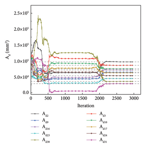
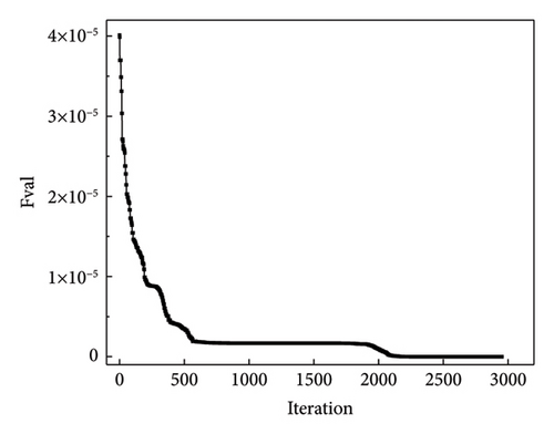
In substructure L, there are 42 DOFs, and the number of DOFs for the unknown displacement is 22. From Section 2, the dimensions of matrix K^′ for the calculation of the unknown displacements are 22 × 42. Matrix K^′ can be calculated based on the information of the partial model L. Subsequently, analytical strains were calculated based on equation (11). The values of the analytical and measured strains were introduced into the objective function to optimize the cross-sectional areas of the members. In this study, two optimization methods were used: the Nelder–Mead simplex (NM) method and the quasi-Newton (QN) method. The NM simplex method uses a simplex consisting of n + 1 points for an n-dimensional vector, x [39]. It is a search method that uses only functional calculations. The NM simplex method is independent of gradient information and is low cost to compute. This method has been widely used. Figure 6(a) shows the variation in the optimized values with the number of iteration steps when the NM simplex method was used. The dotted lines represent the reference lines for the actual condition. The dotted line in the latter part of the text has the same meaning and is not repeated. Figure 6(b) illustrates the variations in the objective function value. Figure 6 demonstrates that the optimized values eventually converge to the “as-is” values of the damaged members. The objective function value eventually converges to zero.

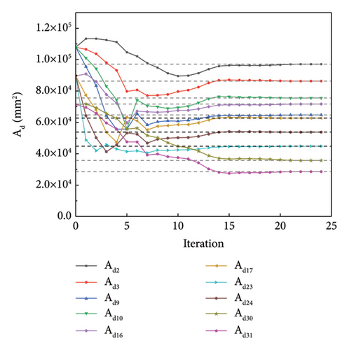
The QN method constructs curvature information based on the observed behavior of f(x) and ∇f(x) in order to approximate the Hessian matrix H using an appropriate update method [40, 41]. The advantage of the QN method is that it does not require the computation of second-order derivatives, which makes the computation cheaper and more efficient. It has advantages in large-scale optimization problems. Figure 7(a) shows the changes in the optimized values during the iteration process when using the QN method. Figure 7(b) shows the change in the function value for each iteration. It can be observed that using the QN method, when the iteration is terminated, the optimized values converge well to the “as-is” values of the members, and the objective function value converges to zero.

The mean relative error (MRE) is a commonly used measure of the accuracy of an estimation method [42]. When the MRE is closer to zero, the difference between the predicted and true values is smaller, and the model is more accurate. Conversely, when the MRE is large, there is a large difference between the predicted results of the model and the true values, and the model is less accurate. In this study, the value was obtained using the following formula:

$$ ()

where M is the total number of damaged members. $$ and $$ represent the optimized and “as-is” cross-sectional areas, respectively. Figure 8(a) and b shows the MRE values of the NM simplex and QN methods during the iteration process, respectively. At the end of each iteration, the final convergence of the MRE value is zero. Therefore, the final optimized values are accurate.

3.2. Middle Region Damage Identification

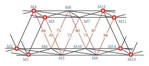
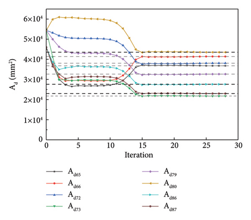
If the damage is concentrated in the middle region, loads can be applied to this region to increase the response of the structure. Loads were applied in the Z direction of nodes 21 and 22 at a magnitude of 100 kN. Similarly, it was assumed that damage occurred in the diagonal members of the truss bridge. The “as-is” cross-sectional areas after member damage are recorded in Table 3. This region is isolated using displacement sensors. The displacement sensors were located at nodes 17–20 and 27–30, as shown in Figure 9(a). The nodes of partial model M are numbered as shown in Figure 9(b). As shown in Figure 9(b), the red members were damaged. Because the node displacements are known at the locations where the displacement sensors were installed, the number of DOFs for the unknown displacements in the partial model M was 18. The dimension of the partial model’s matrix K^′ is 18 × 42. The damage can then be quantified using partial model-based parameter estimation, as described in Section 2.

Table 3. “As-is” cross-sectional area on the middle side of the structure.

Member numbering	Cross-sectional area (mm2)	Member numbering	Cross-sectional area (mm2)
65	36,800	66	41,400
72	38,080	73	21,760
79	32,640	80	43,520
86	27,600	87	23,000

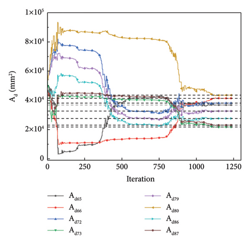
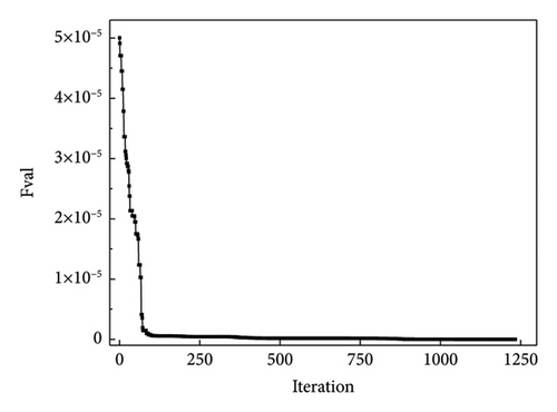
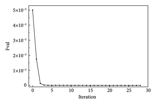
Similarly, the NM simplex and QN methods were used for optimization. Using the NM simplex method, Figure 10(a) shows the change in the parameter values with iterations. Figure 10(b) shows the convergence history of the objective function. As shown in Figure 10, the optimized values eventually converge to the actual values of the members after the damage, and the objective function converges to zero. Figures 11(a) and 11(b) display the convergence processes for the parameters and function value using the QN method, respectively. After fewer iteration steps, the function converges to zeros and the optimized values converge to the “as-is” condition.

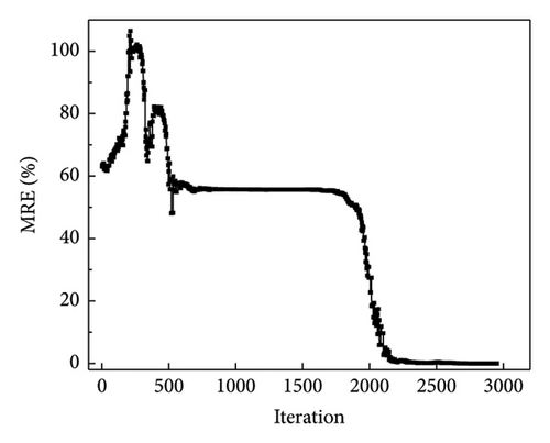
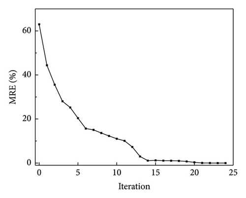
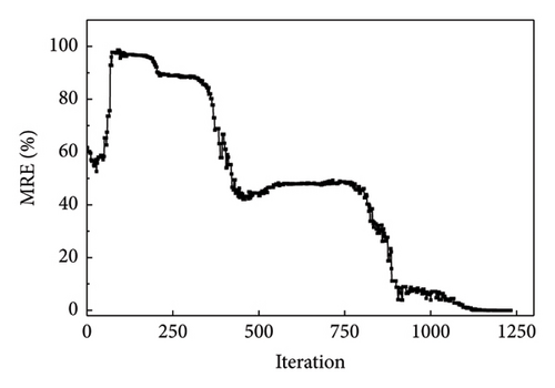
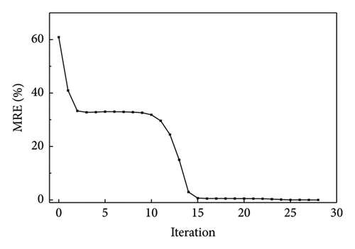
To assess the error between the optimized and actual values, the dotted line plots of the change in the MRE value during the iteration of the two algorithms were plotted separately, as shown in Figure 12. Figure 12(a) shows a plot of the change in MRE values during the optimization process of the NM simplex method, and Figure 12(b) shows that of the QN method. The MRE value was finally close to zero. Therefore, the recognition is deemed excellent.

3.3. Right Region Damage Identification

Assuming that the damage was concentrated in the right region, 100 kN loads were applied at nodes 37 and 38 in the Z direction, as shown in Figure 13(a). In this study, damage identification of the diagonal members and end posts in the right region was performed. The “as-is” cross-sectional areas of the damaged members are shown in Table 4. Because one end contained boundary constraints, the right region could be isolated by installing displacement sensors only on the left side. The region to be identified was named substructure R, which showed that the number of DOFs for unknown displacements was 24. Therefore, the dimension of the partial model’s matrix K^′ is 24 × 42. The strain sensors were located on the damaged members, as shown in Figure 13(b).

Table 4. “As-is” cross-sectional area on the right side of the structure.

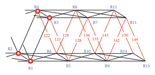
Member numbering	Cross-sectional area (mm2)	Member numbering	Cross-sectional area (mm2)
121	57,139.2	122	49,996.8
128	35,840	129	53,760
135	71,680	136	80,640
142	75,532.8	143	86,323.2
149	64,742.4	150	43,161.6

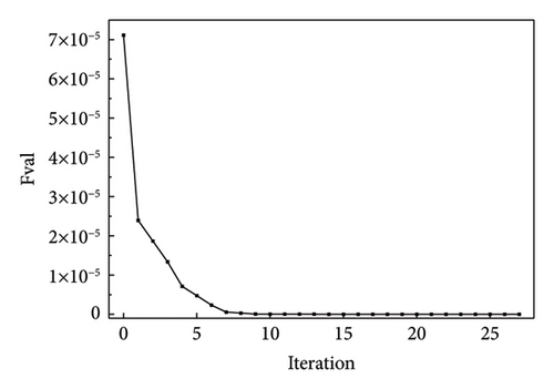
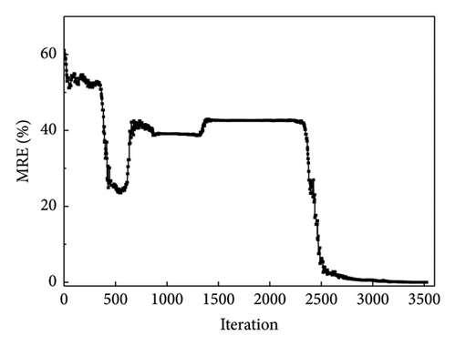
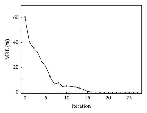
Figures 14 and 15 plot the changes in the optimized and objective function values during the iteration process when using the NM simplex and QN methods for parameter identification, respectively. Both methods eventually converge to the “as-is” condition, and the function value is approached to be 0 with iterations. The MRE value changes during the iteration process are shown in Figure 16(a), which is a plot of the change in MRE values during the optimization process of the NM simplex method, and Figure 16(b) shows that of the QN method. The MRE values eventually approximated zero; therefore, the accuracy of the identified values is high.

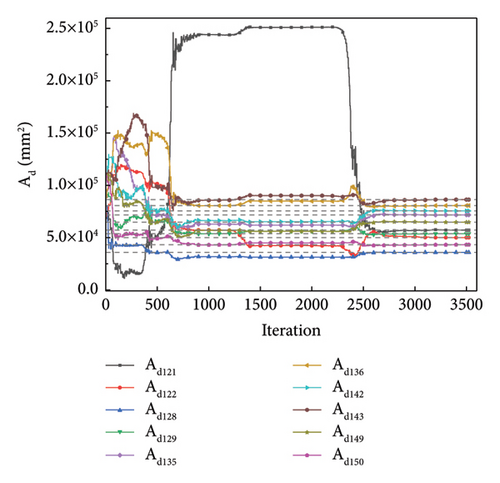
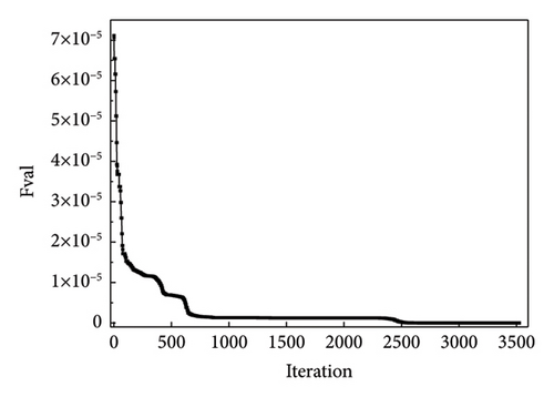
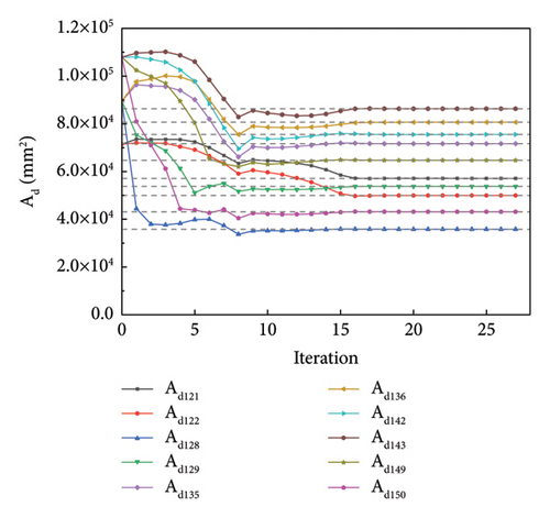
Both the NM simplex and the QN method can be successfully realized for parameter estimation, and the final optimization values converge to the “as-is” condition. The number of iteration steps and final values of the two methods is listed in Table 5. According to the table, the QN method required fewer steps to converge than the NM simplex method. The number of iterative steps of the NM simplex method was significantly greater than that of the QN method. For substructures L, M, and R, the QN method takes only 0.8%, 1.8%, and 0.8% iteration steps of the NM method, respectively. Therefore, in this study, the QN method was more efficient for optimization calculations.

Table 5. Comparison of two algorithms.

Damage region	Optimization method	Iteration step	Final value of function
Substructure L	NM simplex method	2,964	1.36 × 10−15
	QN method	24	1.36 × 10−15
Substructure M	NM simplex method	1,553	8.78 × 10−16
	QN method	28	1.28 × 10−16
Substructure R	NM simplex method	3,522	2.89 × 10−15
	QN method	27	3.99 × 10−17

Next, the number of elements required to assemble the stiffness matrix is discussed. Table 6 shows the dimensions of stiffness matrices based on the different parameter estimation methods. For the general static parameter estimation method, the DOFs of the overall structure are 138, and the size of the overall structure stiffness matrix is 138 × 138. The number of elements contained in the overall structure stiffness matrix is 19,044. For the partial-model-based parameter estimation method, substructures L, M, and R contain 42 DOFs, and their stiffness matrices have the same number of columns. However, their corresponding rows are different, since the number of unknown displacement DOFs is different for each case. The number of elements required to assemble for substructure L, M, and R is 924, 756, and 1,008, respectively. Compared with the general static method, the partial modeling method reduced more than 90% of elements for assembly. The modeling complexity is significantly simplified.

Table 6. Comparison of the sizes of matrices.

Parameter estimation	Region	Size	Element number	Reduction
General static	Overall	138 × 138	19,044	—
Partial-model-based	Left	22 × 42	924	95.1%
	Middle	18 × 42	756	96.0%
	Right	24 × 42	1,008	94.7%

4. Conclusions

This paper proposes a partial-model-based damage identification method that utilizes a stiffness separation technique to address the challenges in detecting damage in long-span truss bridges. In this study, the stiffness of the truss members was analyzed to determine the stiffness influence coefficients that only affect the stiffness of the damaged region and then assembled into the partial model matrix. The equilibrium equation is then established using the known displacements and forces of the damaged region. The analyzed displacements of the unknown DOFs were then solved using inverse analysis. The analytical strains can be obtained from the node displacements at the ends of the members. The analytical values were combined with the measured strain values to establish an objective function for optimization.

A full-size steel truss railroad bridge was used for the analysis. Three representative regions are considered: cases that contain structural left or right constraint boundaries and a case that does not contain structural constraint boundaries. Two algorithms were chosen for the optimization analysis. The results show that damage could be identified in all three cases, whereas all diagonal members and end posts in the identified region were correctly identified. Thus, the proposed method can accurately quantify the damage at the element level and is not limited by the selected identified region. Finally, the iteration efficiencies of the two optimization algorithms were analyzed. Between the NM simplex and QN methods, the QN method has a higher optimization efficiency in these cases.

In summary, the stiffness separation method can be used for damage identification in long-span steel truss bridges. The proposed method does not require complete structural information and only depends on the partial model information, which reduces the size of the matrices required to be assembled. Based on the proposed method, the process of equilibrium equation establishment is significantly simplified. Meanwhile, the proposed method can be applied to space truss roof structures and other types of long-span bridges. The specific analyses for those structures will be further investigated. Additionally, the error in the measurements and loads can impact the accuracy of the damage identification. As future developments, the effect of the measurement and applied load error will also be investigated for the proposed method.

Conflicts of Interest

The authors declare that they have no conflicts of interest.