1. Introduction

Aerodynamics is one of the main forces acting on rockets during flight, and accurate calculation of aerodynamic parameters is beneficial for improving the guidance accuracy of rockets. In the preliminary design stage, numerical calculations [1] and wind tunnel tests [2] are often used in engineering to obtain the aerodynamic characteristics of the aircraft and provide them in the form of interpolation tables. Therefore, aerodynamic parameter identification based on flight test data has important engineering application value. The existing parameter identification algorithms mainly include the least squares method, maximum likelihood method, Kalman filtering, and intelligent algorithms. The following will introduce the research progress of these methods in the field of aerodynamic parameter identification.

The least squares method has a simple form and fast convergence speed and is widely used in aerodynamic parameter identification. Mohamed et al. [3] introduced a total least squares method based on SVD decomposition and applied it to aerodynamic parameter identification. Shaghoury et al. [4] proposed a batch least squares identifier to estimate the parameters of aircraft in icing. Wang et al. [5] proposed a segmented parameter identification approach, using the least squares method to obtain high-precision identification results of lateral aerodynamic parameters. However, the least squares method did not consider the internal noise of the system and did not estimate the system state variables.

The maximum likelihood method, proposed by Fisher, has the characteristics of unbiased, asymptotic consistency, and good convergence. It is a classic identification algorithm for aerodynamic parameter identification. Kumar and Rao [6] used the output error method in the maximum likelihood method to identify the stability derivative of the aircraft and combined it with the cross-validation method to analyze the identification accuracy. Lichota et al. [7] used the maximum likelihood method to achieve aerodynamic identification of rotating projectiles in the wavelet domain, and the results were superior to those in the time domain. However, the maximum likelihood method uses iterative algorithms and takes a long time to calculate, so it is not suitable for online parameter identification.

Kalman filtering can significantly improve the sensor measurement noise output after filtering [8]. Kalman filter can only be used for state estimation of linear systems at first and then developed extended Kalman filter (EKF) and UKF which can be used for state estimation and parameter estimation of nonlinear systems. Ahmad et al. [9] designed a state-dependent Kalman filter (SDKF) based on quasilinear decomposition for unmeasurable state estimation of underground coal gasification. The conventional Taylor series expansion method can be inadequate in case of arbitrary operating points, but this algorithm can accurately approximate nonlinear systems at any operating point. Majeed and Indra [10] used adaptive unscented Kalman filtering to study the identification results of aerodynamic parameters under different process noises. When changing the statistical characteristics of noise, adaptive unscented Kalman filtering outperformed UKF in terms of convergence speed and accuracy. Sun and Xin [11] used high-order volumetric Kalman filtering to estimate the state of hypersonic reentry vehicles and compared it with extended EKF and UKF. Its estimation accuracy and convergence speed were better than those of EKF and UKF. Seo et al. [12] solved aerodynamic parameter identification under abnormal flight conditions using UKF, considering hysteresis effects. Muhammad and Ahsan [13] used UKF for aerodynamic parameter identification of airships and compared it with the identification results of EKF, indicating that the identification accuracy of UKF is better than that of EKF.

Traditional identification methods require parameter modeling, and it is almost impossible to establish a completely accurate parameter model, resulting in modeling errors. The advantage of intelligent algorithms for parameter identification is that they do not require the modeling of parameters, thereby eliminating modeling errors. In recent years, they have been increasingly applied. Marques and Anderson [14] proposed a method for aerodynamic parameter identification using multiple functionals and FIR neural networks. Roudbari and Fariborz [15] used artificial neural networks to model and identify the aerodynamic system of highly maneuverable aircraft without requiring prior information about the system. Yang and Xia [16] proposed an improved particle swarm optimization algorithm that eliminates the need for actuator observations and avoids the influence of model coupling during identification, and its identification accuracy is superior to traditional particle swarm optimization algorithms. However, intelligent algorithms do not fully utilize the prior information of the system, which may lead to overfitting.

EKF is the most widely used state estimation algorithm for nonlinear systems at present, but it has some defects such as large computation and low estimation accuracy. Compared to EKF, UKF does not require the calculation of the system’s Jacobian matrix and has a second-order or higher accuracy. Because they are suitable for computer recursive calculation, they can be used for online identification of aerodynamic parameters. However, existing research often uses simulation data for offline identification. The measurement errors in actual flight tests and the response of the servo are difficult to fully simulate, and the performance of onboard computers also differs from those used by researchers. To verify the engineering application value of UKF, this paper designed a small solid rocket and implemented online identification of aerodynamic parameters using UKF.

2. Modeling

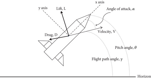
ρ is the density of air. S_ref is the reference area. L_ref is the reference length. C_d is the drag coefficient. C_l is the lift coefficient. C_m is the pitching moment coefficient.

a_x is the axial acceleration. a_y is the normal acceleration. ε is the noise.

δ_e is the elevator angle. δ_e = (δ₁ + δ₂ − δ₃ − δ₄)/4. $$, and $$ means dimensionless pitch angular rate. $$ are the parameters to be identified.

3. The Unscented Kalman Filter

UKF accurately captures the mean and covariance up to the second order of Taylor series expansion for any nonlinear system [17]. The core of UKF is to recursively update the state and covariance of a nonlinear model through a nonlinear transformation—unscented transformation (UT). The principle of UT is to take certain point sets, called sigma points, from the original state distribution according to a certain rule to characterize the input distribution or some statistical characteristics, that is, to make the mean and covariance of these points equal to the mean and covariance of the original state distribution. UKF algorithm can be divided into two steps: the prediction step and the correction step. In both steps, the same UT is used for the system state model and measurement model.

x(t) is the state vector, z(t) is the observation vector, and u(t) is the control input. w(t) is system noise, v(t) is observation noise, they are zero mean Gaussian white noise, and their covariance matrix is Q and R.

χ_i,k−1 is the sampling point, $$ is variance weight, and $$ is mean weight, where λ = α²(L + κ) and L is a scaling parameter. α determines the spread of the sigma points around $$ and is usually set to a small positive value (e.g., le − 3). κ is a secondary scaling parameter which is usually set to 0, and β is used to incorporate prior knowledge of the distribution of x (for Gaussian distributions, β = 2 is optimal).

4. Identification Examples

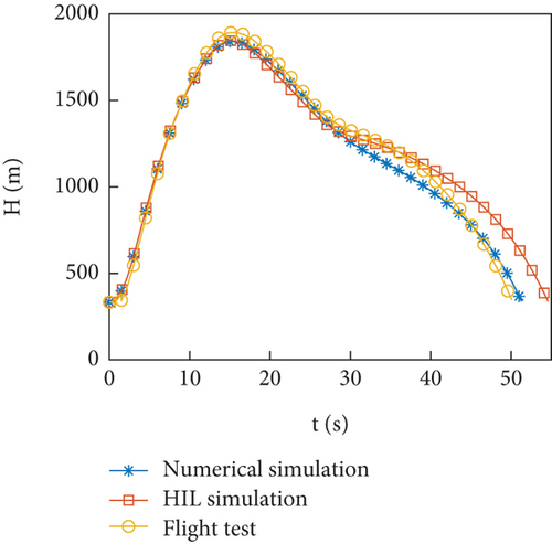
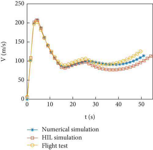
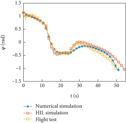
In this section, simulation examples, HIL simulations, and flight test data were identified to verify the effectiveness of parameter identification. The problem in identification was discussed. The flight profile is shown in Figures 2(a)–2(c). The flight trajectory of numerical simulation, HIL simulations, and flight test is similar. The maximum altitude of rocket flight is approximately 1800 m. In the unpowered flight segment selected for parameter identification, the maximum overload of the test rocket is 2 g.

4.1. Numerical Simulation

The aerodynamic force is interpolated by the aerodynamic coefficient interpolation table obtained from the numerical calculation, and the six degrees of freedom trajectory of rocket simulation is carried out. Expanding the parameters to be identified into the system state vector, the state vector is shown as follows.

$$ ()

Using equation (1) as the state equation of UKF and equation (3) as the observation equation, the parameters can be identified by updating the estimation of x based on UKF.

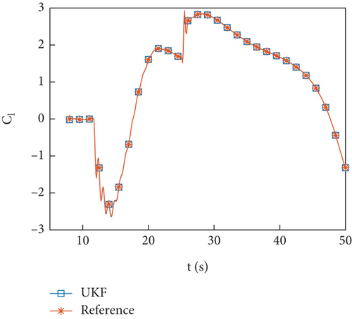
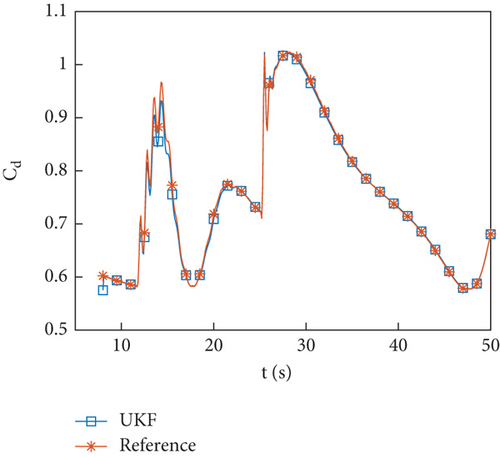
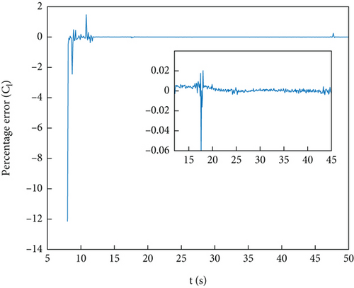
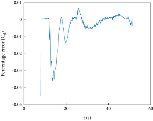
Add Gaussian white noise to the simulation value to simulate the observation value of integrated navigation. The sampling frequency is consistent with the flight test, which is 10 Hz. Figures 3(a)–3(c) show the identification curve of the simulation data, and Figures 4(a) and 4(b) show the percentage error in identification of simulation data. As shown in Figure 3(c), under closed-loop control, the pitching moment coefficient oscillates around 0, making identification difficult. This paper will not discuss the identification of pitching moment. The lift coefficient and drag coefficient are identified well. Since part of the reference value of the lift coefficient is near 0, a large value will appear when calculating the percentage error, but most of the errors are within 1%, so the identification accuracy is high. The percentage error of drag coefficient identification is less than 5%, and after filtering is stable, it is less than 1%.

Figures 5(a)–5(d) show the identification curves of aerodynamic parameters. The reference value is the result of the least squares fitting of aerodynamic force according to equation (4). The identification error of aerodynamic parameters is larger than the error of aerodynamic coefficients, which is caused by modeling error. The identified aerodynamic parameters are near the reference value, with a deviation of no more than 6% from the reference value except for $$. The control system has a certain degree of robustness, and the identified aerodynamic parameters meet the accuracy requirements. The identification error of $$ is significant, and this problem will be discussed in Section 4.4.

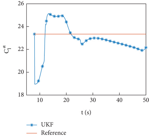
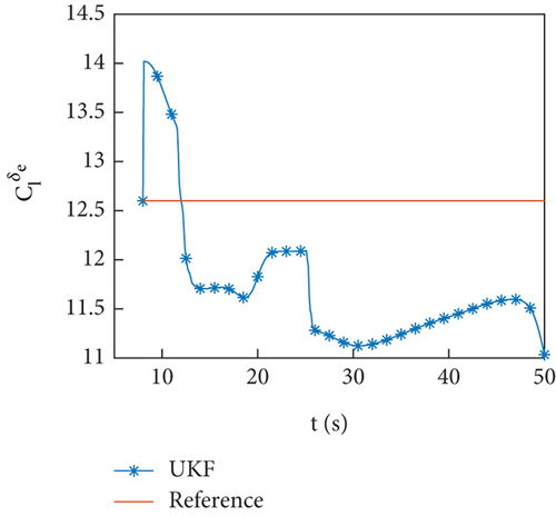
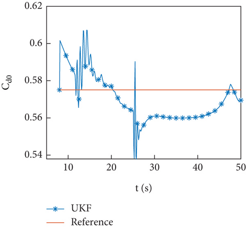
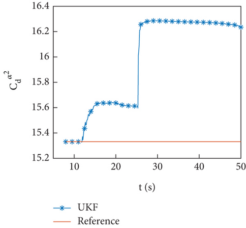
Simulation examples show that the identification scheme proposed in this paper is feasible.

4.2. HIL Simulation

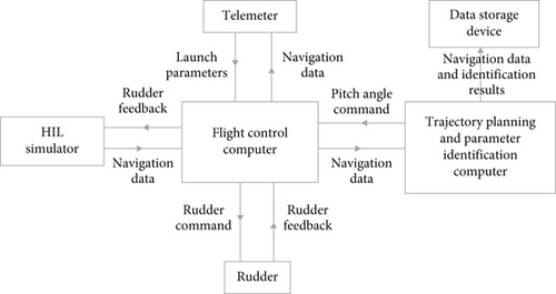
To ensure the normal operation of the identification program on the rocket, this experiment designed the HIL simulation. Figures 6 and 7 show the real-time simulation platform and communication diagrams of the HIL simulation. The HIL simulator and rudder provide discrete and analog signal inputs, which are then calculated by the identification computer and output to the data storage device.

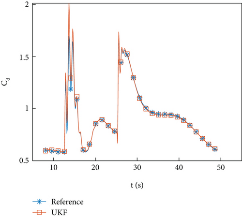
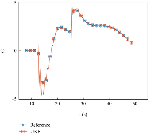
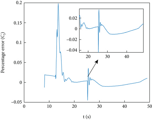
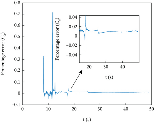
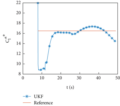
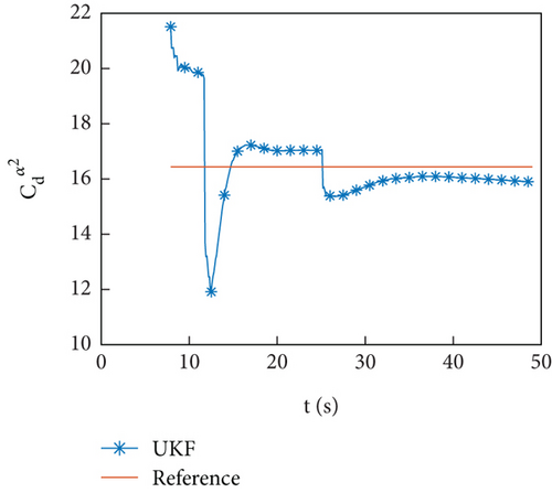
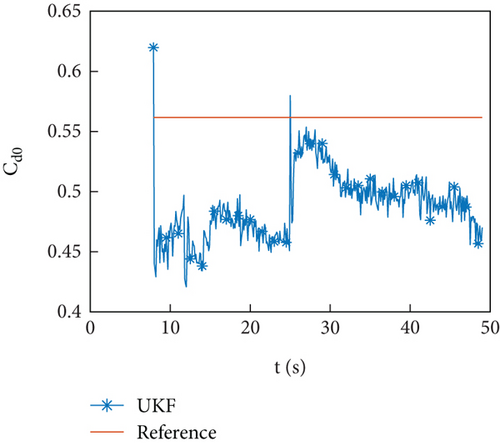
Figures 8(a) and 8(b) and 9(a) and 9(b) show the identification curve and percentage error of the HIL simulation data. The starting time for identification is 7 seconds, and after 15 seconds, which is 7 seconds after filtering, the identification error is within 5%. Except for the time when the guidance program switches at 25 seconds, the error does not exceed 2%. The identification error is within an acceptable range.

Figures 10(a)–10(d) show the identification curves of aerodynamic parameters. The identification errors of C_d0 and $$ are within an acceptable range. The identification errors of $$ and $$ are significant, and this problem will be discussed in Section 4.4.

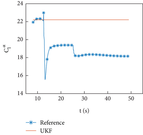
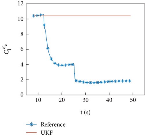
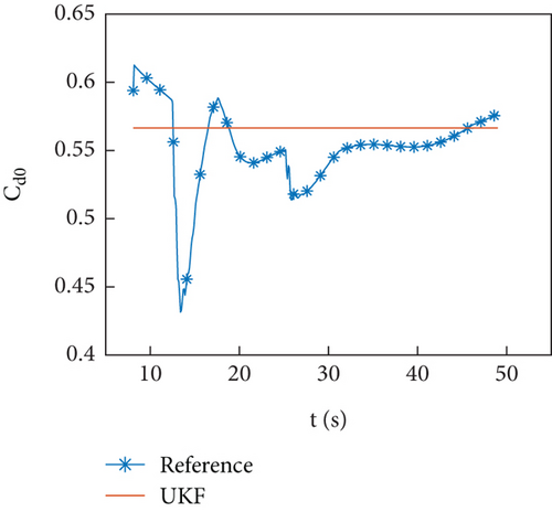
The example of the HIL simulation verifies the identification ability of the identification program under the conditions of using an onboard computer and the presence of servo response.

4.3. Flight Test

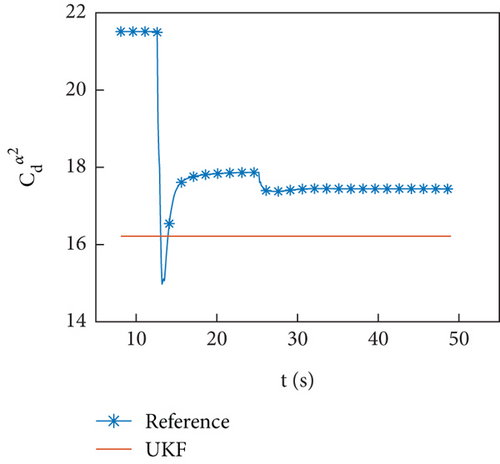
The equipment used in the flight test is consistent with the HIL simulation, but the navigation data is provided by the integrated navigation equipment. Figures 11(a)–11(f) show the identification curves of the flight data. There is a certain deviation between the aerodynamic coefficient filtering results and the reference value, but the trend of change is consistent. The identification method used in this article is still effective and the filtering results will not diverge under real navigation error conditions. However, since the reference values are interpolated based on the aerodynamic coefficient table and there are also certain errors in the numerical calculation of the aerodynamic coefficient table, this article uses trajectory reconstruction to evaluate the identification effect of aerodynamics.

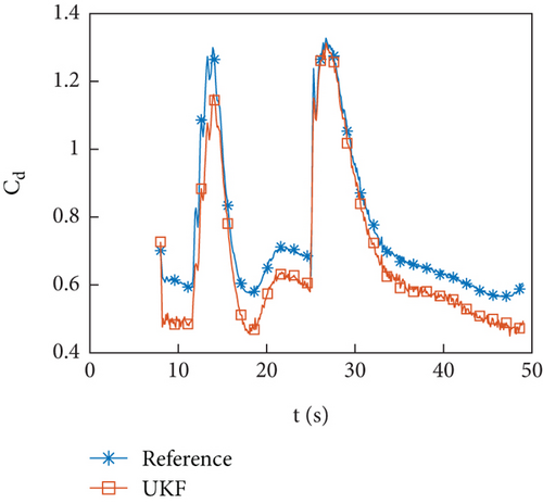
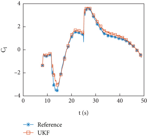
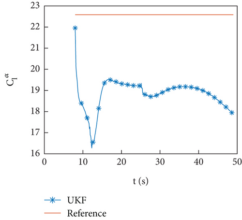
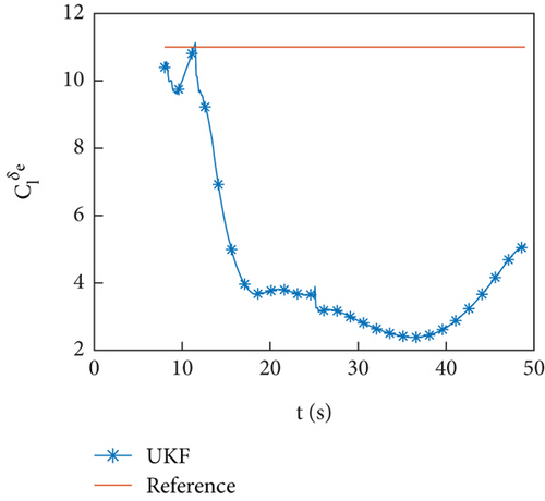
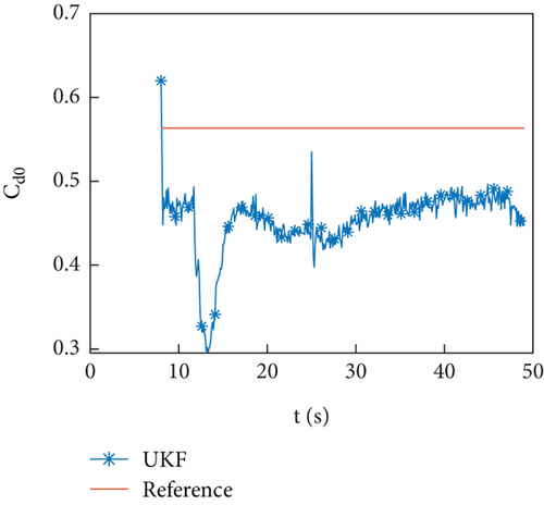
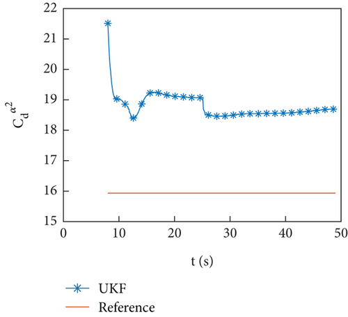
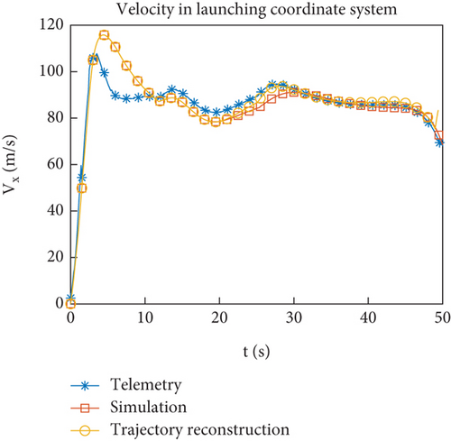
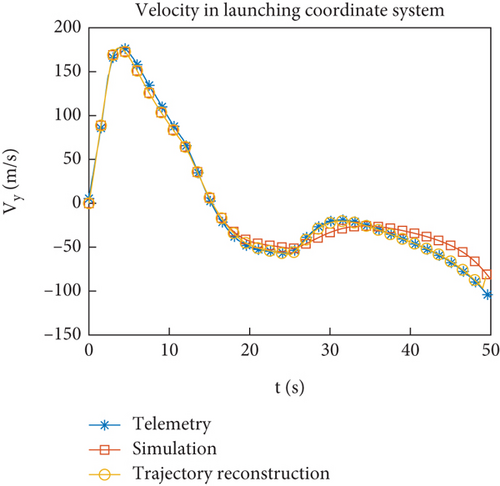
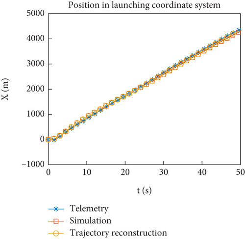
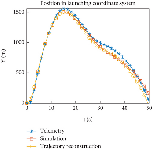
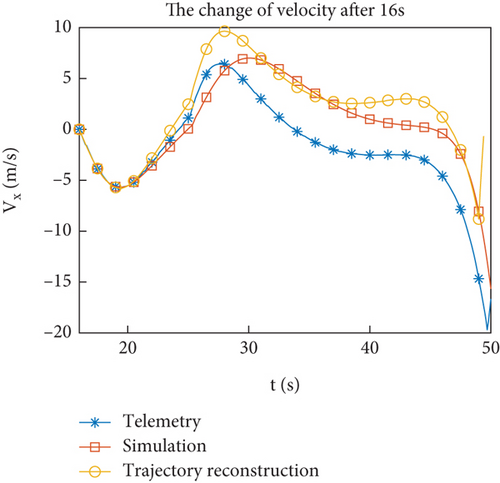
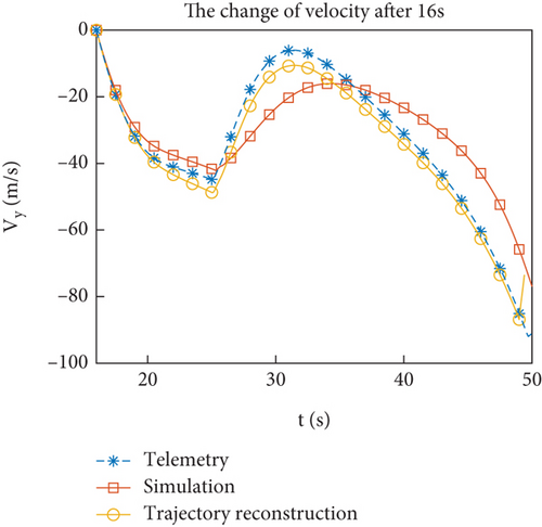
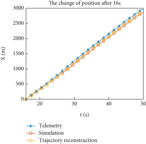
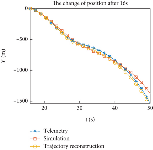
Figures 12(a)–12(h) show the comparison of reconstructed trajectory using identified aerodynamic forces with simulation and telemetry trajectories. Figures 11(e) and 11(f) show that the filtering tends to stabilize after 16 s. When reconstructing the trajectory, the identified aerodynamic force is only used after 16 s, and the aerodynamic coefficient interpolation table is still used before 16 s. Compared to the simulated trajectory, the reconstructed trajectory is closer to the flight trajectory. To avoid the accumulation of errors before 16 s, Figures 12(e)–12(h) show the change of flight state after 16 s, and the comparison effect is more obvious. From the results of trajectory reconstruction, the identification results are effective and superior to the interpolation results of the aerodynamic coefficient table. The identified aerodynamic forces are closer to the real aerodynamic characteristics than numerical calculations.

4.4. Problem and Solution

From the previous identification analysis, it was found that the errors in the identification of $$ and $$ are significant. Figures 13(a)–13(c) show the attack angle and rudder angle curves. It was found that there is an approximately linear relationship between the angle of attack and the rudder angle:

$$ ()

Substitute equation (10) into equation (4):

$$ ()

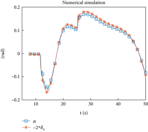
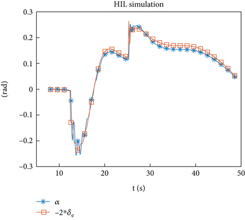
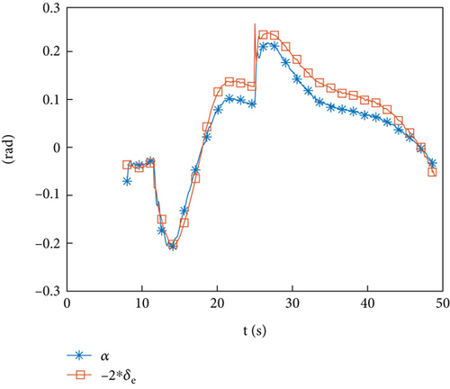
Due to the approximate linear correlation between $$ and $$, there are difficulties in identification.

The rotational motion of rockets is a short period motion, and the sampling period in this article is relatively long, which is 0.1 seconds. Then, the instantaneous equilibrium assumption is satisfied:

$$ ()

$$ and $$ are the derivatives of the pitching moment on the angle of attack and rudder angle. Their values vary within a small range, so

$$ ()

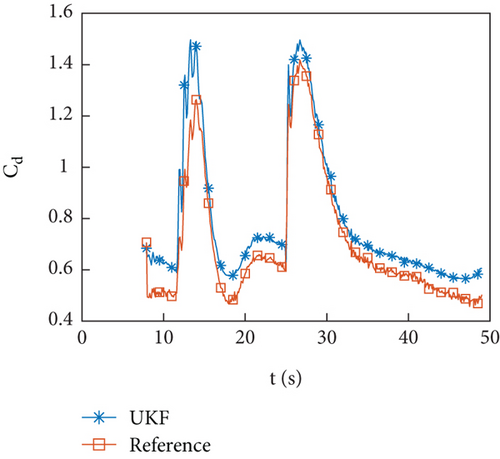
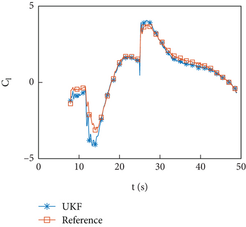
To solve this problem, it can be considered to increase the sampling frequency to capture the time history of A and F changes more accurately. In this flight test, the identification computer was equipped with a trajectory planning program, which requires a large amount of computation. Therefore, the sampling frequency is set to 10 Hz. In addition to increasing the sampling frequency, $$ can be used for identification, and δ_e can be considered to vary with α, which will be effective in control. Following this approach, data stored on storage devices can be used to identify. The results are shown in Figures 14(a)–14(e). From the identification results of $$, it shows that the proposed problem can be solved through this strategy.

5. Conclusions

Conflicts of Interest

The authors declare that there is no conflict of interests regarding the publication of the paper.