Simultaneous Model Change Detection in Multivariate Linear Regression With Application to Indonesian Economic Growth Data
Abstract
In this paper, we study asymptotic model change detection in multivariate linear regression by using the Kolmogorov–Smirnov function of the partial sum process of recursive residuals. We approximate the rejection region and also the power function of the test by establishing a functional central limit theorem for the sequence of the partial sum processes of the recursive residuals of the observations. When the assumed model is true, the limit process is given by the standard multivariate Brownian motion which does not depend on the regression functions. However, when the assumed model is not true (some models change), the limit process is represented by a vector of deterministic trend plus the standard multivariate Brownian motion. The finite sample size rejection region and the power of the test are investigated by means of Monte Carlo simulation. The simulation study shows evidence that the proposed test is consistent in the sense that it attains the power larger than the size of the test when the hypothesis is not true. We also demonstrate the application of the proposed test method to Indonesian economic growth data in which we test the adequacy of three-variate low-order polynomial model. The test result shows that the growth of the Indonesian economy is neither simultaneously constant nor linear. The test has successfully detect the appearance of a change in the model which is mainly caused by the COVID-19 pandemic in 2020.
1. Introduction
As stated in Fujikoshi [1], He et al. [2], Somayasa [3], and Somayasa, Ruslan, and Sutiari [4], multivariate linear regression has been applied in many fields of study including agriculture, economics, geology, biology, and chemistry, among others. One important part of statistical modelling using multivariate linear regression is checking whether each component of the mean of the response vector can be adequately represented by a set of regression functions or whether we need more functions to represent some components of the mean of the response vector. This intention can be realized in practice by conducting simultaneous detection whether there are some changes in regression model. Cotos-Yéñez, Pérez-González, and González-Manteiga [5], Fujikoshi [1], and Zimmerman [6] called this step as model check. In other literatures, it also frequently called goodness of fit test for regression (see Das [7]).
Methods for change detection in multivariate linear regression has been intensively studied. They are commonly developed based on the residuals of the responses. Likelihood ratio test using modified Wilk’s lambda statistic has been documented in the literatures of multivariate linear regression (cf. [1, 2]). This method is applicable only when the response vector is normally distributed. Somayasa et al. [8] developed asymptotic model check method for multivariate linear regression with spatial observations on a compact rectangle based on the partial sum process of the vector of ordinary least squares residuals. The limit process obtained in [8] has been derived analytically by using some transformation theorems and the linear property of the partial sum operator. However, as it can be seen therein, the limit process appeared as an intricate function of the standard multivariate Brownian motion. It depends not only on the design of experiment but also on the assumed regression functions. By this reason, the quantiles of the Kolmogorov–Smirnov as well as the Cramér–von Mises type test statistics can not be computed analytically. This clearly restricted the application of the proposed method in practice. Although the limit process has a complex structure, nevertheless it is geometrically interpretable as a projection of the standard multivariate Brownian motion on its kernel space. This simple structure gives advantage in analyzing the power of the test when the assumed model is not true (see Somayasa [9]).
Partial sum method has been initially investigated for the purpose of quality monitoring in production process. The application of the method has been continuously developed to the problem of monitoring structural change for regression by defining a test based on the partial sum process of recursive residuals. Recent publications related to this context are Jiang and Kurozumi [10], Dao [11], and Otto and Breitung [12], among others. Groen, Kapetanios, and Price [13] pioneered the extension of the application of the method for monitoring structural change in multivariate linear regression based on the partial sum process of the vector of recursive residuals. However, their approaches required a normal distribution assumption attached to the vector of the errors, so that they are not purely asymptotic in the strictly sense. When the vector of random errors in the model is multivariate normally distributed, then the vector of recursive residuals builds a sequence of mutually independent random vectors, so that the limit distribution of the corresponding sequence of the partial sum processes of the vector of recursive residuals can be immediately obtained. This means that the application of the method in the practice must be started with a goodness of fit test or diagnostic check regarding the normality of the vector of recursive residuals.
In this paper, we study the application of the partial sum process of multivariate recursive residuals in asymptotic model check for multivariate linear regression defined on a closed and bounded experimental region. For that, we need to establish a functional central limit theorem for the partial sum process of recursive residuals obtained from multivariate linear regression under more general setting then that defined in Groen, Kapetanios, and Price [13]. It is worth mentioning that the results presented in [10–13] have been derived solely for univariate times series linear regression, where the experimental region is given by the set of positive integers which is not closed and bounded. In contrast to time series, when the experimental region is compact, we have triangular arrays of observations. For that, we need to establish a functional central limit theorem applied to triangular arrays of observations drawn from a multivariate linear regression model. To the knowledge of the authors, this result has not been yet documented elsewhere. It will require more effort on one hand by the existence of the correlation among the components of the response vector, but on the other hand, linear regression is attractive statistical tool which is applied in many areas such as in response surface methodology, chemical industry, and mining industry, among others.
The paper is organized as follows. In Section 2, we discuss literature review. Multivariate regression model with univariate experimental region together with the definition of the test statistic for checking the adequacy of the model is defined in Section 3. The limit process of the sequence of the partial sum processes of recursive residuals is investigated in Section 4 for the situation under H0 as well as under H1. The proofs of the results are postponed to the appendix. Section 5 discusses the results of numerical simulation. In Section 6, we demonstrate the application of the proposed test method to real data which is the Indonesian economic growth data. Some conclusions and remarks are presented in Section 7.
2. Literature Review
Model check or model change detection plays important role in every serious empirical model building for a random phenomenon. As in geostatistics, Bassani and Costa [14] informed that optimum prediction (kriging) of the spatial process in unobserved geographical positions depends on the adequateness of a proposed regression model. Myers, Montgomery, and Anderson-Cook [15] stated that in response surface methodology, the validity of an assumed regression model determines the level of accuracy of the optimum condition of a production process under study. This means that to be able to obtain accurate prediction result, we have to carry out model change detection before the assumed model is used in the prediction (see also Huang and He [16]).
As documented in Fahrmeir et al. [17] and Zimmerman [6], model check or model change detection in multivariate liner regression can be conducted in several various ways: graphical method, Akaike information criterion (AIC), and likelihood ratio test by making use of Wilk’s lambda statistic. All methods have similar approach in that they are conducted by investigating the residuals of the observations. As a classical method, the decision obtained by graphical method is subjective so that this method is rarely used in the practice. AIC and likelihood ratio test are two inferential methods that have drawback in the application in that they are conducted under the assumption that the observations are normally distributed (see Fujikoshi [1] and He et al. [2]).
Bischoff and Gegg [18] proposed a purely asymptotic test method for detecting change in multivariate linear regression based on the partial sum process of ordinary least squares residuals. This innovative approach successfully incorporates the theory of high-dimensional stochastic process especially high-dimensional Gaussian process in the statistical inference. Many authors proposed test method based on the partial sums of recursive residuals instead of ordinary least squares residuals. Recently, Dao [11] studied the application of this approach for condition monitoring and fault diagnosis of wind turbines. Jiang and Kurozumi [10] investigated the power properties of the test based on the modified partial sum process of recursive residuals. Otto and Breitung [12] applied the partial sum method for testing and monitoring structural change of COVID-19.
To the best knowledge of the authors, the only work that investigated the application of the partial sum process of recursive residuals obtained from multivariate linear regression observed over time is that written by Groen, Kapetanios, and Price [13]. As it has been already mentioned in Section 1, they derived the limit process under multivariate normally distributed random error which clearly restricted the application of the method. Motivated by [13], in this work, we propose asymptotic test method based on the partial sum process of recursive residuals with application to simultaneous model change detection in multivariate linear regression of Indonesian economic growth data.
As defined in Bonokeling et al. [19], economic growth is an increase in the production of economic goods and services in one period of time compared with a previous period. Economic growth of a country reflects and measures the ability of the government in developing the economy of the corresponding country. Economic growth is commonly measured in terms of the increase in aggregated market value of additional goods and services produced which is measured based on the gross domestic product (GDP).
According to the study documented in Sari [20] and Febriyanti [21], there are at least four variables that frequently influence the economic growth of a country, namely, investment, government expenditure, export, and import. Each variable has a different impact on economic growth. While investment, government spending, and export positively affect economic growth, import negatively affects economic growth.
As it has been quoted in [19], other factor that can cause negative influence to the economic growth is disaster, such as COVID-19 outbreaks. The COVID-19 has destroyed world economy in 2020 which has brought the world to worst economic recession. Indonesia is one of more than 210 countries in the world that has been hit by the COVID-19 pandemic. Muhyiddin and Nugroho [22] reported that this situation has caused the Indonesian economic grew negatively in the second, third, and fourth quarters of 2020 after a positive growth achieved in the first quarter of 2020. In this work, we aim to check asymptotically that the COVID-19 causes change in the model of the Indonesian economic growth so that it can not be modelled anymore using low-degree polynomial over time.
3. Model Definition
It is clear that the wider the dispersion of the assumed model to the true-unknown model, the larger the value of will be. This means that the statistic in Equation (9) measures the discrepancy between the true and the assumed model. By this reason, can be reasonably used as a test statistic in detecting the occurrence of some changes in the model. We will reject H0 when is large. For that, the limit distribution of under H0 as well as under H1 needs to be investigated.
We notice that the partial sum process (Equation 8) differs to those defined in [13] in that they did not include the rest term of Equation (8) in their definition. Consequently, the process defined in [13] has sample path in the space of p-dimensional right continuous functions on D with left limit, denoted by , instead of the space .
4. Approximation to the Test Statistics
Since the exact distribution of is mathematically not tractable, we investigate their limit distribution. We firstly obtain the limit process of Qn−m(Up×(n − m)) by applying Theorem 7.5 of Billingsley [23] (see also Theorem 1.5.4 of Van der Vaart and Wellner [24]).
Thus, builds a sequence of uncorrelated p-dimensional random vectors with and . If the random error vector is distributed as Np(0, Σ), then unj is also distributed as Np(0, Σ). Hence, under such condition, the set constitutes a sequence of independent and identically distributed random vectors.
Now we are in the position to state the limit distribution of under H0. The proof is given in the appendix.
Theorem 1. Let the regression functions s1, ⋯, sm be linearly independent in L2(P, D), continuous, and have bounded variation on D. Suppose that , for i = 1, ⋯, p, n ≥ 1 and j = m + 1, ⋯, n. If H0 is true, then for n⟶∞, converges in distribution to Bp. Thereby, Bp is the standard p-variate Brownian motion on D. That is, a centered p-variate Gaussian process with the covariance function given by
We consult the reader to Durrett [25] for the definition of the standard p-variate Brownian motion Bp.
This means that Equation (16) is computed based on the p-dimensional ordinary least squares residuals.
The limit process of , for when H0 is not true, is summarized in Theorem 2. The proof is postponed to the appendix.
Theorem 2. Let the regression function s1, ⋯, sm be linearly independent in L2(P0, D), continuous, and have bounded variation on D. Suppose that the model
When H0 is true, the power computed in Equations (20) and (21) will reduce to the probability of type I error of the test of size α. Conversely, when H0 is not true, both determine the probability of the rejection of H0 provided that g is a true regression function vector. In other words, and Ψ(g) supply information regarding the ability of the test in detecting the existence of model change. A good test should own the general property stated in Lehmann and Romano [26] and Rasch and Schott [27]. That is, the larger the power under H1 is, the better is the test.
5. Numerical Simulation
Polynomial model clearly satisfies the condition of Theorem 1.
5.1. Simulation Under H0
The simulation result for n = 40 is devoted in Figure 1, where Figure 1(a) is for x = 0.5 and Figure 1(b) is for x = 1. The graph of the empirical cumulative distribution function (ECDF) of the quadratic form of the three-variate RRPSP is scattered using the step line. The curve indicated by the dotted line is for the cumulative distribution function (CDF) of χ2(3). All graphs are generated using R under 10000 runs. In the second scenario, we simulate three-variate quadratic model (m = 3) defined on the unit interval [0, 1]. The error vectors are generated independently from the three-variate centered normal distribution having the same covariance matrix as in the first case. The graphs of the ECDF of the quadratic form of the RRPSP simulated for n = 40, x = 0.5, and x = 1 together with the graphs of the CDF of χ2(3) are presented in Figures 2(a) and 2(b), respectively.
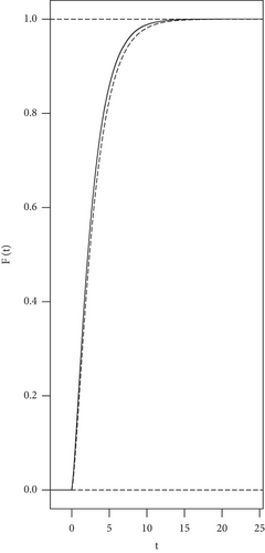
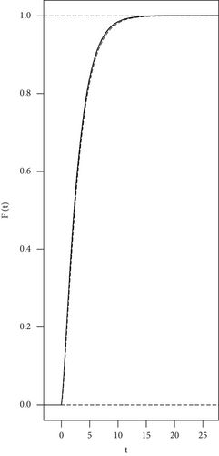

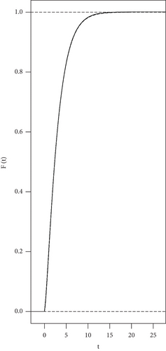
The simulation results show that independent to the proposed regression model and to the chosen value of x ∈ {0.5, 1}, χ2(3) gives a good approximation to the distribution of the quadratic form of the three-variate RRPSP.
Table 1 consists of the simulated lower quantiles of for α = 65%, 75%, 85%, 90%, 95%, and 99%, simulated for n = 25, 30, 35, 40, 45, and 50, under 100000 runs. These quantiles are used in constructing the finite sample size rejection region of the test. The R coding for generating the graphs and the lower tail quantiles can be obtained by request to the authors.
| n | |||||
|---|---|---|---|---|---|
| p = 2 | |||||
| 25 | 1.9229 | 2.1770 | 2.3591 | 2.6438 | 3.2097 |
| 30 | 1.9263 | 2.1794 | 2.3583 | 2.6389 | 3.2043 |
| 35 | 1.9270 | 2.1839 | 2.3680 | 2.6518 | 3.2108 |
| 40 | 1.9305 | 2.1822 | 2.3639 | 2.6415 | 3.1978 |
| 45 | 1.9362 | 2.1909 | 2.3712 | 2.6423 | 3.1923 |
| 50 | 1.9282 | 2.1829 | 2.3618 | 2.6444 | 3.1902 |
| p = 3 | |||||
| 25 | 2.2615 | 2.5203 | 2.6999 | 2.9738 | 3.5337 |
| 29 | 2.2611 | 2.5176 | 2.6971 | 2.9763 | 3.5235 |
| 35 | 2.2693 | 2.5232 | 2.7050 | 2.9893 | 3.5511 |
| 40 | 2.2643 | 2.5208 | 2.7018 | 2.9770 | 3.5278 |
| 45 | 2.2674 | 2.5241 | 2.7038 | 2.9840 | 3.5250 |
| 50 | 2.2690 | 2.5218 | 2.6988 | 2.9785 | 3.5211 |
| p = 4 | |||||
| 25 | 2.4970 | 2.7477 | 2.9298 | 3.2032 | 3.7301 |
| 30 | 2.4979 | 2.7499 | 2.9302 | 3.1978 | 3.7332 |
| 35 | 2.5054 | 2.7545 | 2.9303 | 3.2013 | 3.7448 |
| 40 | 2.5075 | 2.7605 | 2.9392 | 3.2172 | 3.7514 |
| 45 | 2.5121 | 2.7672 | 2.9456 | 3.2205 | 3.7544 |
| 50 | 2.5174 | 2.7699 | 2.9490 | 3.2157 | 3.7573 |
5.2. Simulation Under H1
When the constants ρ, γ, and δ are simultaneously set to zero, the condition under H0 is fulfilled which means that there are no changes in the model. In such a case, the power of the test should be equal to the size of the test 5%. However, when at least one of these constants are nonzero, then there exists some i ∈ {1, 2, 3} such that . In other words, there exist some models that change simultaneously.
- 1.
H11: (when ρ ≠ 0, γ = 0, and δ = 0)
- 2.
H12: (when ρ = 0, γ ≠ 0, and δ = 0)
- 3.
H13: (when ρ = 0, γ = 0, and δ ≠ 0)
- 4.
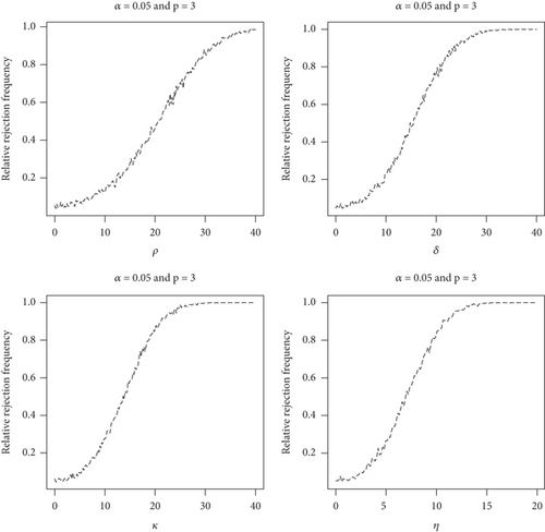
H14: for all i = 1, 2, 3 attained when ρ ≠ 0, γ ≠ 0, and δ ≠ 0. It can be seen therein that when ρ = 0, γ = 0, and δ = 0, the power of the test attains the value 0.04967 for n = 30 and attains the value 0.05340 for n = 40, which are approximately equal to 5%. So the size of the test is achieved. The graphs of the simulated power function of size 5% test associated with the alternatives H11, H12, H13, and H14 are scattered in Figure 3 simulated for n = 40 under 10000 runs. The graphs indicate increasing power functions. They have a common feature in that the larger the values of ρ, γ, and δ are, the greater the powers. All powers reach the size of the test at the starting points, that is when ρ, γ, and δ are simultaneously fixed to zero. Tables 2 and 3 and Figure 3 show that the power of the test for such alternatives gets large as the model moves away from H0. This means that the test has good power in detecting the existence of some changes in the model when some changes exist. By referring to Ghosh, Delampady, and Samanta [28], it can be concluded based on the simulation results that the test is unbiased
| ρ | γ | δ | ρ | γ | δ | ||
|---|---|---|---|---|---|---|---|
| n = 30 | |||||||
| 0.0 | 0.0 | 0.0 | 0.0497 | 0.0 | 0.0 | 0.5 | 0.0495 |
| 4.5 | 0.0 | 0.0 | 0.0576 | 0.0 | 0.0 | 2.5 | 0.0609 |
| 10.5 | 0.0 | 0.0 | 0.0875 | 0.0 | 0.0 | 5.5 | 0.1091 |
| 12.5 | 0.0 | 0.0 | 0.1109 | 0.0 | 0.0 | 8.5 | 0.2079 |
| 14.5 | 0.0 | 0.0 | 0.1340 | 0.0 | 0.0 | 12.5 | 0.4353 |
| 16.5 | 0.0 | 0.0 | 0.1622 | 0.0 | 0.0 | 15.0 | 0.6061 |
| 20.0 | 0.0 | 0.0 | 0.2259 | 0.0 | 0.0 | 20.0 | 0.8722 |
| 25.0 | 0.0 | 0.0 | 0.3434 | 0.0 | 0.0 | 25.0 | 0.9801 |
| 30.0 | 0.0 | 0.0 | 0.4911 | 0.0 | 0.0 | 30.0 | 0.9985 |
| 40.0 | 0.0 | 0.0 | 0.7722 | 0.5 | 0.5 | 0.5 | 0.0526 |
| 0.0 | 0.5 | 0.0 | 0.0516 | 2.5 | 2.5 | 2.5 | 0.0948 |
| 0.0 | 4.0 | 0.0 | 0.0735 | 3.5 | 3.5 | 3.5 | 0.1405 |
| 0.0 | 10.5 | 0.0 | 0.2512 | 5.5 | 5.5 | 5.5 | 0.3228 |
| 0.0 | 15.0 | 0.0 | 0.4995 | 6.5 | 6.5 | 6.5 | 0.4430 |
| 0.0 | 20.0 | 0.0 | 0.7810 | 8.5 | 8.5 | 8.5 | 0.7035 |
| 0.0 | 30.0 | 0.0 | 0.9917 | 10.0 | 10.0 | 10.0 | 0.8540 |
| 0.0 | 35.0 | 0.0 | 0.9994 | 12.5 | 12.5 | 12.5 | 0.9725 |
| 0.0 | 40.0 | 0.0 | 0.9999 | 15.0 | 15.0 | 15.0 | 0.9973 |
| ρ | γ | δ | ρ | γ | δ | ||
|---|---|---|---|---|---|---|---|
| n = 40 | |||||||
| 0.0 | 0.0 | 0.0 | 0.0534 | 0.0 | 0.0 | 0.5 | 0.0497 |
| 4.5 | 0.0 | 0.0 | 0.0576 | 0.0 | 0.0 | 2.5 | 0.0590 |
| 10.5 | 0.0 | 0.0 | 0.0913 | 0.0 | 0.0 | 5.5 | 0.1047 |
| 12.5 | 0.0 | 0.0 | 0.1063 | 0.0 | 0.0 | 8.5 | 0.1995 |
| 14.5 | 0.0 | 0.0 | 0.1290 | 0.0 | 0.0 | 12.5 | 0.4215 |
| 16.5 | 0.0 | 0.0 | 0.1586 | 0.0 | 0.0 | 15.0 | 0.5840 |
| 20.0 | 0.0 | 0.0 | 0.2153 | 0.0 | 0.0 | 20.0 | 0.8565 |
| 25.0 | 0.0 | 0.0 | 0.3366 | 0.0 | 0.0 | 25.0 | 0.9754 |
| 30.0 | 0.0 | 0.0 | 0.4747 | 0.0 | 0.0 | 30.0 | 0.9973 |
| 40.0 | 0.0 | 0.0 | 0.7576 | 0.5 | 0.5 | 0.5 | 0.0533 |
| 0.0 | 0.5 | 0.0 | 0.0493 | 2.5 | 2.5 | 2.5 | 0.0958 |
| 0.0 | 4.0 | 0.0 | 0.0742 | 3.5 | 3.5 | 3.5 | 0.1450 |
| 0.0 | 10.5 | 0.0 | 0.2431 | 5.5 | 5.5 | 5.5 | 0.3167 |
| 0.0 | 15.0 | 0.0 | 0.4744 | 6.5 | 6.5 | 6.5 | 0.4339 |
| 0.0 | 20.0 | 0.0 | 0.7723 | 8.5 | 8.5 | 8.5 | 0.6818 |
| 0.0 | 24.0 | 0.0 | 0.9244 | 10.5 | 10.5 | 10.5 | 0.8393 |
| 0.0 | 30.0 | 0.0 | 0.9912 | 12.5 | 12.5 | 12.5 | 0.9681 |
| 0.0 | 35.0 | 0.0 | 0.9988 | 15.0 | 15.0 | 15.0 | 0.9963 |
6. Application
The matrix indicates the existence of strong correlations among the three variables. These tendencies are also visualized graphically in Figure 4 which is the scatter matrix of the data. The strongest correlation appears between the total value of investment and the GDP, namely, 0.90174, whereas the weakest correlation is that between the total value of export and the GDP, that is, 0.67968. By reviewing this fact, the statistical analysis of the three variables must be handled simultaneously applying multivariate method.

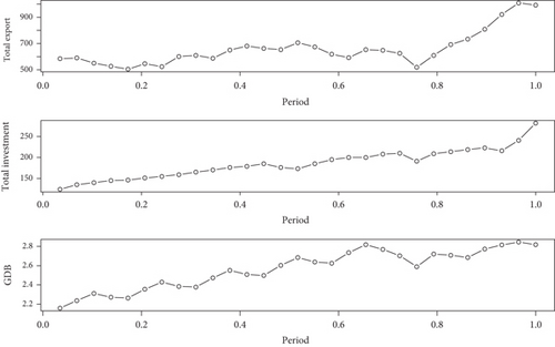
We aim to model the data using three-variate polynomial regression model and conduct a test for checking the adequacy of a proposed model based on the partial sum process of the recursive residuals. For that we interpret, the data as a realization of 29 independent three-dimensional vector responses admitting three-variate regression model observed on equidistance design points {1/29, 2/29, ⋯, 1} over the unit interval [0,1]. The scatter plot of the total value of investment, the total value of export, and the GDP are presented in Figure 5. The existence of deep peaks in the scatter plot of the data appeared as the impact of the contraction of the Indonesia’s economic growth during the COVID-19 pandemic in 2020. In the normal situation, the total values of export, import, and the GDP should smoothly increase so that they can be modelled by means of lower degree polynomial functions. We infer that the COVID-19 pandemic will change the model in which they need to be modelled by means of higher degree polynomial model. The existence of these changes will be detected by using the proposed test procedure. The computation result of the test statistic for several low-order three-variate polynomial regression models is presented in Table 4. The R coding for computing can be obtained by request to the author. Since the lower 95% quantile of the distribution of for n = 29 and p = 3 takes the value 2.9763 (see Table 1), then the asymptotic size 5% test will reject constant model and first-order model, whereas second-order model and third-order model will not be rejected. The test result seems to be synchronous with the scatter plot of the data in that constant and first-order models are not plausible for the Indonesia’s economic growth data during the period of March 2020 until March 2022.
| Model | Critical value |
|---|---|
| Constant | 9.3802 |
| First order | 3.0876 |
| Second order | 1.8136 |
| Third order | 2.8870 |
7. Conclusion
A limit theorem for the sequence of a random function defined by the RRPSP of multivariate linear regression has been established. The result can be applied in detecting the existence of changes in regression model. In the case of no change, we successfully obtain the limit. It has been given by the standard multivariate Brownian motion {Bp(x): x ∈ D} which is a model free limit process which depended only on the dimension of the response vector. When there exists at least one change, the limit process has been obtained as a vector of trends plus the standard multivariate Brownian motion, that is, {hG(x) + Bp(x): x ∈ D}. We have built simulation to approximate the finite sample size critical values as well as the power of the Kolmogorov–Smirnov type test. The simulation showed that the test based on the multivariate RRPSP leads to an unbiased test with good power. This test method can be implemented in computer using statistical package like R, so that the computation is quite fast.
Conflicts of Interest
The authors declare no conflicts of interest.
Funding
This work was supported in part by the Indonesian Ministry of Research, Technology and Higher Education through the KLN and Publikasi Internasional Research Grant 2019.
Appendices
Proof of Theorem 1
Proof of Theorem 2
We notice that the p × p symmetric matrix ∫[0, z]s(u)s⊤(u)P0(du) is invertible since the columns are linearly independent (see also Somayasa and et al. [8]), establishing the proof.
Open Research
Data Availability Statement
The PDF data used to support the findings of this study were supplied by BPS under license and so cannot be made freely available. Requests for access to these data should be made to Wayan Somayasa ([email protected]).


