Risk Assessment for Complex Systems Based on Fuzzy Cognitive Maps: A Case of the Biopharmaceutical Industry
Abstract
Analyzing the supply chain (SC) of biopharmaceutical drugs can be challenging due to their complexity, the existence of a wide variety of risks, and the dynamics of the system. This paper presents a framework for evaluating the SC risks of Iranian biopharmaceutical companies based on cause-and-effect relationships and fuzzy cognitive maps (FCMs). We first interviewed several biopharmaceutical supply experts to learn about potential SC risks, causal relationships among FCM concepts, FCM structure, and FCM activation cycle. The most critical and relevant risks and significant elements of the SCs, such as cost, time, and quality, were identified as relevant FCM concepts. Then, we used failure mode and effects analysis (FMEA) and the FCM of the SC risks to assess the impacts of the biopharmaceutical SC risks on each other and on the crucial elements of the SCs. The Hebbian learning algorithms were then applied to train the FCM models. We tested different scenarios to evaluate the impacts of FCM concepts on the SC risks. The proposed approach can prioritize risk factors and, more importantly, predict and analyze the effect of each risk factor/risk group on other risks or the outcome of a given risk. The proposed FCM features and the knowledge gained from evaluating them can provide practical and helpful information to pharmaceutical companies to deal with their supply risks more efficiently.
1. Introduction
Biopharmaceutical products are essential in restoring health and saving lives worldwide. The biotechnology industry has made Iran a leader in the biotechnology market in the Middle East and North Africa [1]. Based on Iranian pharmaceutical statistics, domestically generated biopharmaceuticals accounted for over 11 percent of the Iranian medication market share in 2020.
When defining risk across various domains, adopting a multidisciplinary approach is imperative as it allows for the consideration of a multitude of factors, thereby facilitating a more comprehensive approach to risk analysis [2]. Multidisciplinary risk assessment frameworks that integrate techniques from fields such as operations’ research, decision science, and artificial intelligence can provide holistic insights into complex risk landscapes. Recent studies [2, 3] have demonstrated the value of combining methodologies such as fuzzy cognitive mapping, failure mode and effects analysis, and quality function deployment in enhancing risk assessments across sectors such as manufacturing, supply chains, and distribution processes. By drawing from diverse domains, these integrative approaches capture a wider range of risk factors and their intricate interdependencies, leading to more informed risk mitigation strategies. The findings demonstrate that combining multiple multicriteria decision-making (MCDM) techniques and synthesizing their outcomes enhances confidence in risk assessments and failure mode rankings, while effectively handling uncertainties and divergent expert judgments [4]. The decomposed fuzzy set (DFS) failure mode and effects analysis (FMEA) approach accounts for uncertainties and indecision in decision-makers’ evaluations by allowing them to provide assessments for risk occurrence, severity, and detectability from both optimistic and pessimistic perspectives [5].
Managing supply chain (SC) risks is a significant challenge in the field of SC management [6, 7]. Biopharmaceutical SCs face unique challenges, including supply variations [8], demand fluctuations [9], disruptive events [10], production uncertainty [11], and other factors [12, 13]. Recent advances in various biopharmaceuticals and their sensitive nature have increased the complexity of SCs for these drugs, posing new challenges for decision-makers [14]. Also, the uncertainties in the production process of biological pharmaceuticals set their SCs apart from those of chemical drugs [15, 16]. The most critical players in drug SCs are pharmaceutical manufacturers [17]. Their performance affects the efficiency of the entire process, and their significant investments in research and development and responsibility for the quality of the final products put them at higher risk than others. Therefore, drug manufacturers are in the best position to identify and manage SC risks [18].
Quality (product or service), cost, and time are the most important indicators of business performance [19]. Drug SC management aims to benefit patients and the health system by delivering high-quality products and services to end-users (patients) at the right time, cost, and location [20]. Thus, gaining a clear understanding of drug SC risks is essential to improve the efficiency of drug SCs and reduce potential risks and flaws. Prior research predominantly employed conventional quantitative/qualitative tools such as analytic hierarchy process (AHP) [21, 22]. These methods exhibit static dependencies among logical variables, lacking consideration for process variables, time, uncertainties, and human behavior [23, 24]. Consequently, they fall short in evaluating the dynamic risks inherent in these systems. Common risk analysis tools, such as failure mode and effects analysis (FMEA) [25, 26], fault tree analysis [27], analytic hierarchy process [28], and the analytic network process [29], are not able to accurately predict risk behavior and perform dynamic risk analysis. Therefore, existing tools cannot be used for an accurate assessment of the SC risks of biopharmaceutical companies.
Fuzzy cognitive maps (FCMs) serve as powerful graphical tools for modeling complex system behaviors [30, 31]. Within the framework of an FCM, nodes represent key concepts of a system, while the weights assigned to links quantify the strength of relationships between these concepts. The evolution of FCMs has seen various definitions and developments aimed at enhancing performance, interpretation, prediction, and modeling capabilities. FCMs boast advantageous features such as fuzzy reasoning, straightforward structure, high flexibility, and trainability, capturing the attention of numerous researchers [32]. The effectiveness of the FCM method is well-documented across diverse decision-making applications, as evidenced by a plethora of studies [29–33]. Particularly, noteworthy is its successful application in risk analysis within decision-making contexts. For instance, Zarrin’s evolutionary algorithm for constructing FCM models and inferring genetic causal networks showcases the method’s versatility in addressing intricate problems [33]. In the mining industry, Samadi et al. applied FCM to assess postclosure strategies, integrating evidential reasoning to contribute to sustainable mining policy [34]. FCM has also demonstrated its efficacy in tackling challenges within production processes. Jahangoshai Rezaee et al.’s study, employing FCM in conjunction with failure mode and effects analysis, successfully identified and prioritized failures in a food production process [35]. This integration of FCM with other methodologies underscores its adaptability and effectiveness in addressing real-world problems. Irannezhad et al. delved into the use of FCM to model causal relationships and assess blockchain readiness within the sphere of SC management [36]. This research exemplifies FCM’s applicability in evaluating and enhancing the resilience of SCs. Similarly, Mzougui et al. utilized FCM to organize knowledge related to human risk management, demonstrating its utility in comprehensively addressing challenges in industrial environments [37]. Furthermore, FCMs are commonly employed in risk analysis [3].
In summary, these studies collectively highlight the versatility and effectiveness of the FCM method in addressing intricate decision-making problems across diverse domains. The expansion of biopharmaceutical production in Iran, coupled with challenges in drug SCs, particularly in biopharmaceutical supply, inefficiencies in traditional risk analysis methods, and the capabilities of FCM, motivated us to leverage the FCM technique for estimating SC risks within Iranian biopharmaceutical companies. The FCM employed in this study can be refined through the use of active Hebbian learning (AHL) and nonlinear Hebbian learning (NHL) algorithms.
2. Materials and Methods
This study delves into the SC risks faced by biopharmaceutical companies in Iran, marking the first exploration of its kind. The research focuses on unraveling the cause-and-effect relationships between these risks, with the study population comprising biopharmaceutical companies registered by the Iranian Food and Drug Administration. The methodology involves a three-phase FCM-based approach for drug SC risk management.
Phase I: Identification of drug supply chain risks.
- (i)
Initial Identification. Conducting a systematic review to pinpoint SC risks.
- (ii)
Interviews with Experts. Engaging in semistructured interviews with industry experts, particularly those well-versed in biopharmaceuticals. Questions cover risks across different regions and phases of the biopharmaceutical SC.
- (iii)
Categorization. Organizing identified risks into macrorisks, supply risks, organization- and strategy-related risks, demand risks, financial risks, support risks, and regulatory risks.
- (iv)
Fuzzy Screening. Experts rate identified risks based on their industry significance using fuzzy numbers (FNs).
- (i)
Questionnaire Design. Developing a questionnaire to gather expert opinions on the mutual impact of concepts. Linguistic variables and fuzzy sets represent impact levels.
- (ii)
Graph FCM. Creating a specific FCM to explore causal relationships between concepts (risks and goals), treating risks and goals as nodes in the system.
- (iii)
Initial Weights. Calculating the arithmetic mean of expert responses for each element. The center-of-gravity defuzzification method yields nonfuzzy weights for links in the FCM graph.
- (i)
Risk Activation. Determining the initial value of risk-related concepts based on the risk priority number (RPN) from failure mode and effects analysis.
- (ii)
Scenario Testing. Defining various scenarios, such as simultaneous activation of all risks, group activation, and individual activation, with initial values based on risk scores.
- (iii)
FCM Training. Employing NHL and AHL algorithms to enhance FCM performance by iteratively updating numerical weights.
- (iv)
Analysis. Examining the effects of different scenarios on SC variables (time, cost, and quality) and levels of other risks.
2.1. Fuzzy Screening
By implementing a threshold, we prioritize risks of higher importance over others. In line with the suggested hypothesis, factors with geometric means below the threshold were excluded. The threshold, denoted as α, was established at α = 0.8θ. In this formula, θ represents the difference between the maximum and minimum values of the non-FN. In this study, α = 0.8θ = 0.8 (4.87−1.12) = 3. Consequently, if Mc ≥ α, the risk is acknowledged as significant; otherwise, the risk is considered not very high [24].
2.2. FCM Structure
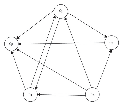
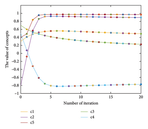
Equation (4) shows an FCM inference. ci(k) denotes the value of the concept ci in the kth iteration and ci(k − 1) is its value in the (k − 1)th iteration. Also, f(⋅) represents a transfer function, the most common forms of which are the sigmoid and the hyperbolic functions [37]. Figure 1 shows an example of a hypothetical FCM with six concepts, whose transfer function is of the hyperbolic tangent type. Figure 1(a) illustrates the FCM graph, and Figure 1(b) shows the results of the FCM inference.
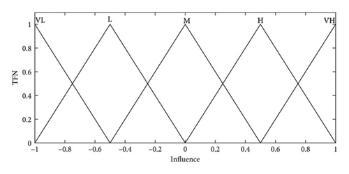
A questionnaire was designed, and experts were asked to comment on the impact of the concepts on each other using linguistic variables. The effect of concept is expressed by the linguistic variables very low (VL), low (L), moderate (M), high (H), and very high (VH) with corresponding fuzzy sets, as shown in Figure 2.
2.3. FCM Training and Inference

In (8), η2 is the learning rate and η1 is the parameter of weight descent.
The arithmetic mean of all data was calculated for each element after receiving expert feedback. The resulting non-FN (using the center-of-gravity defuzzification method [39]) indicates the weight (initial weight) of the link between the two concepts in the FCM graph. The impact of activating a risk or a collection of risks on other SC risks is investigated in this step. The FCMs are inferred using equation (5), the impact of activation of a risk is investigated by the use of equation (4), and the number of risks associated with a risk being activated is inferred.
Here, D is the probability of risk detection, O is the rate of risk occurrence, CI is the impact on cost, TI is the impact on time, and QI is the impact on quality. To test the diverse scenarios and the FCM inference on these scenarios, we defined 27 scenarios, which included the simultaneous activation of all risks, the activation of risks in groups, and the activation of risks individually. The initial value of the concepts is based on the risk score obtained from the previous steps. To improve FCM performance, we train it using NHL and AHL algorithms. The numerical weights obtained in the second phase by these algorithms are updated at each FCM iteration step. For AHL, the activation cycle is determined by expert opinions. Finally, the effects of various scenarios on the three SC variables of time, cost, and quality, as well as the levels of other risks, are examined.
3. Results
After conducting a review study, 16 biopharmaceutical experts were interviewed. Based on the interviews, the coding, and synchronization of the risks, 16 different items of the risks in the review study were obtained. A total of 95 risks were identified from reviewing sources and interviewing experts. After applying fuzzy screening, 20 high-importance risks in the biopharmaceutical industry were identified. The RPN was used to determine the risk of each failure situation. This number is the product of the multiplication of the risk factors of probability, severity, and detectability, as shown in Table 1.
| Category | Risk | Ranking | Risk score |
|---|---|---|---|
| Macro | Sanction (R2) | 1 | 0.381 |
| Regulatory | Lack of good governance for medicines (R16) | 2 | 0.325 |
| Macro | MOH conflicts of interest (R1) | 3 | 0.311 |
| Financial | Dual exchange rate (R7) | 4 | 0.307 |
| Regulatory | Drug list limitation (R15) | 5 | 0.305 |
| Regulatory | Lobbying risks in the decision-making process (R19) | 6 | 0.303 |
| Regulatory | Inefficient pricing policies (R17) | 7 | 0.298 |
| Financial | Currency fluctuation (R11) | 8 | 0.297 |
| Supply | Defect in the domestic supply of essential raw materials (R4) | 9 | 0.288 |
| Financial | Money transfer problem (R6) | 10 | 0.287 |
| Regulatory | Pseudo-productivity (repacking) (R14) | 11 | 0.280 |
| Financial | Cash flow risk (R10) | 11 | 0.280 |
| Financial | Interest rate (R12) | 12 | 0.231 |
| Financial | Long cash collection cycle (R9) | 13 | 0.230 |
| Financial | Inflation rate (R8) | 14 | 0.208 |
| Regulatory | Change in legislation and policies (R20) | 15 | 0.205 |
| Regulatory | Banking regulation instability (R18) | 16 | 0.204 |
| Organization and strategies’ issues | Defect of international vision (R5) | 17 | 0.190 |
| Macro | Political instability (R3) | 18 | 0.181 |
| Demand | Demand fluctuations (R13) | 19 | 0.170 |
3.1. FCM for Dynamic Risk Assessment
Based on expert opinions and the steps taken, an FCM with 23 concepts is designed. The concepts of c1 to c20 (SC risks) are represented as R1 to R20, respectively. The concepts of c21 to c23, which represent time, cost, and quality, respectively, are represented as P1 to P3. The total number of contact vectors between nodes is 176, and on average, each node is associated with at least seven other nodes (Table 2).
| Index | Value |
|---|---|
| Total components | 23 |
| Total connections | 176 |
| Connection density | 0.3327032 |
| Connections per component | 7.652174 |
| Number of transmitter components | 1 |
| Number of receiver components | 3 |
| Number of ordinary components | 19 |
| Number of no connections | 0 |
| Number of self-loops | 0 |
| Complexity (R/T) | 3 |
The initial weights of the communication links are obtained by defuzzifying expert opinions regarding the causal effect of concepts on each other. These values are presented in Table 3. The NHL algorithm is used to train the FCM at this stage. As suggested by the experts, the FCM activation cycle is such that the R1, R2, and R3 risks are activated first, but not all risks are activated at the same time. Then, the other risks are activated, and finally, the P1, P2, and P3 risks are activated. We also train the FCM designed for SC risks of Iranian biopharmaceutical companies using the AHL algorithm.
| R1 | R2 | R3 | R4 | R5 | R6 | R7 | R8 | R9 | R10 | R11 | R12 | R13 | R14 | R15 | R16 | R17 | R18 | R19 | R20 | P1 | P2 | P3 | |
|---|---|---|---|---|---|---|---|---|---|---|---|---|---|---|---|---|---|---|---|---|---|---|---|
| R1 | 0 | 0 | 0.23 | 0.1 | 0 | 0 | 0 | 0 | 0.27 | 0.24 | 0 | 0 | 0.14 | 0.22 | 0.35 | 0.37 | 0.35 | 0 | 0.42 | 0.28 | 0.15 | 0 | −0.25 |
| R2 | 0.6 | 0 | 0.45 | 0.45 | 0.48 | 0.61 | 0.52 | 0.5 | 0.35 | 0.37 | 0.46 | 0.3 | 0.29 | 0.07 | 0.28 | 0 | 0.25 | 0.35 | 0.2 | 0.23 | 0.46 | 0.41 | −0.45 |
| R3 | 0.13 | 0 | 0 | 0.29 | 0.31 | 0.18 | 0.18 | 0.19 | 0 | 0 | 0.27 | 0.13 | 0 | 0 | 0 | 0.35 | 0.21 | 0.16 | 0.31 | 0.45 | 0.17 | 0.22 | −0.08 |
| R4 | 0 | 0 | 0 | 0 | 0 | 0 | 0 | 0 | 0 | 0 | 0 | 0 | 0 | 0.22 | 0 | 0 | 0 | 0 | 0 | 0 | 0.42 | 0.35 | −0.34 |
| R5 | 0 | 0 | 0 | 0 | 0 | 0 | 0 | 0 | 0 | 0 | 0 | 0 | 0 | 0.23 | 0 | 0 | 0 | 0 | 0 | 0 | 0 | 0 | −0.22 |
| R6 | 0 | 0 | 0 | 0.25 | 0.12 | 0 | 0.23 | 0.32 | 0.16 | 0.29 | 0.25 | 0.19 | 0 | 0 | 0 | 0.14 | 0 | 0.34 | 0.14 | 0.1 | 0.48 | 0.45 | −0.08 |
| R7 | 0.1 | 0 | 0 | 0.25 | 0 | 0.38 | 0 | 0.3 | 0 | 0.24 | 0.35 | 0.18 | 0 | 0.1 | 0 | 0.19 | 0.26 | 0.17 | 0.16 | 0 | 0.29 | 0.2 | −0.22 |
| R8 | 0 | 0 | 0 | 0 | 0 | 0 | 0.19 | 0 | 0.22 | 0.33 | 0.33 | 0.39 | 0.18 | 0 | 0 | 0 | 0.24 | 0.2 | 0 | 0 | 0 | 0.35 | −0.09 |
| R9 | 0 | 0 | 0 | 0.2 | 0 | 0 | 0 | 0 | 0 | 0.51 | 0 | 0 | 0 | 0 | 0 | 0 | 0.09 | 0 | 0 | 0 | 0.34 | 0.34 | −0.08 |
| R10 | 0 | 0 | 0 | 0.24 | 0 | 0.17 | 0 | 0 | 0.22 | 0 | 0 | 0 | 0 | 0 | 0 | 0 | 0 | 0 | 0 | 0 | 0.27 | 0.38 | 0 |
| R11 | 0 | 0 | 0.19 | 0.19 | −0.18 | 0.19 | 0.3 | 0.35 | 0.17 | 0.34 | 0 | 0 | 0 | −0.14 | 0 | 0 | 0.26 | 0.23 | 0 | 0 | 0.16 | 0.31 | −0.19 |
| R12 | 0 | 0 | 0 | 0 | 0 | 0 | 0 | 0.22 | 0 | 0.22 | 0 | 0 | 0 | 0 | 0 | 0 | 0 | 0 | 0 | 0 | 0 | 0.27 | 0 |
| R13 | 0 | 0 | 0 | 0.11 | 0 | 0 | 0 | 0 | 0 | 0 | 0 | 0 | 0 | 0 | 0 | 0 | 0 | 0 | 0 | 0 | 0.15 | 0.1 | 0 |
| R14 | 0 | 0 | 0 | 0.25 | 0.13 | 0 | 0 | 0 | 0 | 0 | 0 | 0 | 0 | 0 | 0 | 0.15 | 0.14 | 0 | 0.23 | 0 | 0 | 0 | 0 |
| R15 | 0.2 | 0 | 0 | 0 | −0.1 | 0 | 0 | 0 | 0 | 0 | 0 | 0 | 0.11 | 0 | 0 | 0.21 | 0 | 0 | 0.25 | 0 | 0 | 0 | 0 |
| R16 | 0.36 | 0 | 0.14 | 0.25 | 0 | 0 | 0 | 0 | 0.1 | 0 | 0 | 0 | 0 | 0.34 | 0.26 | 0 | 0.35 | 0 | 0.48 | 0.32 | 0.21 | 0.23 | −0.28 |
| R17 | 0.1 | 0 | 0 | 0.26 | 0 | 0 | 0 | 0 | 0.19 | 0.25 | 0 | 0 | 0 | 0.13 | 0 | 0 | 0 | 0 | 0.19 | 0 | 0.16 | 0.26 | −0.34 |
| R18 | 0 | 0 | 0 | 0.2 | 0 | 0.32 | 0 | 0 | 0 | 0.31 | 0.15 | 0.22 | 0 | 0 | 0 | 0 | 0 | 0 | 0 | 0 | 0.25 | 0.29 | 0 |
| R19 | 0.33 | 0 | 0 | 0 | 0 | 0 | 0 | 0 | 0 | 0 | 0 | 0 | 0 | 0.24 | 0.22 | 0.3 | 0.28 | 0 | 0 | 0.13 | 0 | 0 | −0.31 |
| R20 | 0.19 | 0 | 0 | 0.12 | 0 | 0 | 0 | 0 | 0 | 0 | 0 | 0 | 0 | 0 | 0 | 0.22 | 0 | 0 | 0 | 0 | 0.14 | 0 | 0 |
| P1 | 0 | 0 | 0 | 0 | 0 | 0 | 0 | 0 | 0 | 0 | 0 | 0 | 0 | 0 | 0 | 0 | 0 | 0 | 0 | 0 | 0 | 0 | 0 |
| P2 | 0 | 0 | 0 | 0 | 0 | 0 | 0 | 0 | 0 | 0 | 0 | 0 | 0 | 0 | 0 | 0 | 0 | 0 | 0 | 0 | 0 | 0 | 0 |
| P3 | 0 | 0 | 0 | 0 | 0 | 0 | 0 | 0 | 0 | 0 | 0 | 0 | 0 | 0 | 0 | 0 | 0 | 0 | 0 | 0 | 0 | 0 | 0 |
3.2. Result of Different Scenarios
At this stage, the inactive risks have an initial value of zero, and the initial value of the active risks is the RPN. The simulation is performed in the MATLAB software environment. The FCM-based simulation process of each scenario ends when consistency in the value of the concepts is achieved. We designed 27 different scenarios in order to assess and interpret the impact of each risk category and also each individual risk factor on the other risks, and Table 4 shows numerical results related to the scenarios, including the initial and final values of concepts and the number of iterations. Table 4 shows the untrained FCM results and the FCM results trained by the NHL.
| Scenario | Description | R1 | R2 | R3 | R4 | R5 | R6 | R7 | R8 | R9 | R10 | R11 | R12 | R13 | R14 | R15 | R16 | R17 | R18 | R19 | R20 | P1 | P2 | P3 |
|---|---|---|---|---|---|---|---|---|---|---|---|---|---|---|---|---|---|---|---|---|---|---|---|---|
| 1 | Activating all risks | 0.311 | 0.381 | 0.181 | 0.288 | 0.190 | 0.287 | 0.307 | 0.208 | 0.230 | 0.280 | 0.297 | 0.231 | 0.170 | 0.280 | 0.305 | 0.325 | 0.298 | 0.204 | 0.303 | 0.205 | 0 | 0 | 0 |
| NHL results (irritation 9) | 0.718 | 0.032 | 0.486 | 0.877 | 0.262 | 0.654 | 0.572 | 0.676 | 0.714 | 0.879 | 0.665 | 0.621 | 0.406 | 0.698 | 0.594 | 0.779 | 0.828 | 0.620 | 0.823 | 0.670 | 0.919 | 0.946 | −0.867 | |
| AHL results (irritation 9) | 0.743 | 0.047 | 0.455 | 0.881 | 0.171 | 0.649 | 0.560 | 0.690 | 0.706 | 0.884 | 0.625 | 0.624 | 0.302 | 0.687 | 0.557 | 0.798 | 0.857 | 0.564 | 0.828 | 0.640 | 0.916 | 0.944 | −0.865 | |
| 2 | Activating macrorisks | 0.311 | 0.381 | 0.181 | 0 | 0 | 0 | 0 | 0 | 0 | 0 | 0 | 0 | 0 | 0 | 0 | 0 | 0 | 0 | 0 | 0 | 0 | 0 | 0 |
| NHL results (irritation 14) | 0.697 | 0.008 | 0.419 | 0.863 | 0.167 | 0.605 | 0.504 | 0.629 | 0.694 | 0.865 | 0.617 | 0.567 | 0.322 | 0.677 | 0.562 | 0.761 | 0.813 | 0.566 | 0.808 | 0.638 | 0.907 | 0.936 | −0.853 | |
| AHL results (irritation 15) | 0.652 | 0.011 | 0.341 | 0.824 | 0.113 | 0.503 | 0.398 | 0.526 | 0.629 | 0.818 | 0.496 | 0.460 | 0.231 | 0.627 | 0.490 | 0.716 | 0.779 | 0.442 | 0.770 | 0.565 | 0.880 | 0.913 | −0.825 | |
| 3 | Activating supply risks | 0 | 0 | 0 | 0.288 | 0 | 0 | 0 | 0 | 0 | 0 | 0 | 0 | 0 | 0 | 0 | 0 | 0 | 0 | 0 | 0 | |||
| NHL results (irritation 6) | 0.004 | 0.000 | 0.001 | 0.015 | 0.001 | 0.000 | 0.000 | 0.000 | 0.002 | 0.003 | 0.000 | 0.000 | 0.000 | 0.010 | 0.003 | 0.006 | 0.006 | 0.000 | 0.008 | 0.004 | 0.016 | 0.014 | −0.016 | |
| AHL results (irritation 6) | 0.004 | 0.000 | 0.001 | 0.015 | 0.002 | 0.000 | 0.000 | 0.000 | 0.002 | 0.003 | 0.000 | 0.000 | 0.000 | 0.010 | 0.003 | 0.006 | 0.006 | 0.000 | 0.008 | 0.004 | 0.016 | 0.014 | −0.016 | |
| 4 | Activating organization and strategies’ risks | 0 | 0 | 0 | 0 | 0.190 | 0 | 0 | 0 | 0 | 0 | 0 | 0 | 0 | 0 | 0 | 0 | 0 | 0 | 0 | 0 | |||
| NHL results (irritation 6) | 0.003 | 0 | 0 | 0 | 0.004 | 0.007 | 0.000 | 0.000 | 0.002 | 0.002 | 0.000 | 0.000 | 0.000 | 0.007 | 0.002 | 0.004 | 0.004 | 0.000 | 0.005 | 0.003 | 0.005 | 0.004 | −0.009 | |
| AHL results (irritation 6) | 0.003 | 0 | 0.001 | 0.004 | 0.007 | 0.000 | 0.000 | 0.000 | 0.002 | 0.002 | 0.000 | 0.000 | 0.000 | 0.007 | 0.002 | 0.004 | 0.004 | 0.000 | 0.006 | 0.003 | 0.005 | 0.004 | −0.009 | |
| 5 | Activating financial risks | 0 | 0 | 0 | 0 | 0 | 0.287 | 0.307 | 0.208 | 0.230 | 0.280 | 0.297 | 0.231 | 0 | 0 | 0 | 0 | 0 | 0 | 0 | 0 | |||
| NHL results (irritation 14) | 0.691 | 0.000 | 0.398 | 0.859 | 0.138 | 0.594 | 0.493 | 0.617 | 0.689 | 0.860 | 0.605 | 0.557 | 0.302 | 0.672 | 0.550 | 0.757 | 0.810 | 0.555 | 0.806 | 0.629 | 0.904 | 0.934 | −0.850 | |
| AHL results (irritation 16) | 0.623 | 0.000 | 0.302 | 0.810 | 0.093 | 0.466 | 0.361 | 0.485 | 0.615 | 0.803 | 0.466 | 0.424 | 0.215 | 0.612 | 0.474 | 0.690 | 0.754 | 0.415 | 0.753 | 0.541 | 0.869 | 0.903 | −0.812 | |
| 6 | Activating demand risks | 0 | 0 | 0 | 0 | 0 | 0 | 0 | 0 | 0 | 0 | 0 | 0 | 0.170 | 0 | 0 | 0 | 0 | 0 | 0 | 0 | |||
| NHL results (irritation 6) | 0.000 | 0.000 | 0.000 | 0.004 | 0.000 | 0.000 | 0.000 | 0.000 | 0.000 | 0.000 | 0.000 | 0.000 | 0.005 | 0.001 | 0.000 | 0.000 | 0.000 | 0.000 | 0.001 | 0.000 | 0.004 | 0.003 | −0.002 | |
| AHL results (irritation 6) | 0.000 | 0.000 | 0.000 | 0.004 | 0.000 | 0.000 | 0.000 | 0.000 | 0.000 | 0.000 | 0.000 | 0.000 | 0.005 | 0.001 | 0.000 | 0.001 | 0.001 | 0.000 | 0.001 | 0.000 | 0.004 | 0.003 | −0.002 | |
| 7 | Activating regulatory risks | 0 | 0 | 0 | 0 | 0 | 0 | 0 | 0 | 0 | 0 | 0 | 0 | 0 | 0.280 | 0.305 | 0.325 | 0.298 | 0.204 | 0.303 | 0.205 | |||
| NHL results (irritation 15) | 0.686 | 0.000 | 0.395 | 0.853 | 0.147 | 0.569 | 0.459 | 0.591 | 0.682 | 0.854 | 0.580 | 0.527 | 0.297 | 0.668 | 0.552 | 0.750 | 0.803 | 0.529 | 0.799 | 0.626 | 0.901 | 0.930 | −0.846 | |
| AHL results (irritation 19) | 0.628 | 0.000 | 0.303 | 0.807 | 0.099 | 0.448 | 0.338 | 0.458 | 0.605 | 0.793 | 0.448 | 0.397 | 0.216 | 0.622 | 0.488 | 0.692 | 0.750 | 0.404 | 0.759 | 0.549 | 0.865 | 0.898 | −0.810 | |
| 8 | Activating risk 1 | 0.311 | 0 | 0 | 0 | 0 | 0 | 0 | 0 | 0 | 0 | 0 | 0 | 0 | 0 | 0 | 0 | 0 | 0 | 0 | 0 | |||
| NHL results (irritation 25) | 0.636 | 0.000 | 0.313 | 0.813 | 0.103 | 0.461 | 0.351 | 0.474 | 0.617 | 0.802 | 0.462 | 0.410 | 0.223 | 0.626 | 0.491 | 0.700 | 0.758 | 0.413 | 0.763 | 0.557 | 0.870 | 0.902 | −0.816 | |
| AHL results (irritation 27) | 0.623 | 0.000 | 0.302 | 0.805 | 0.098 | 0.449 | 0.341 | 0.461 | 0.605 | 0.792 | 0.449 | 0.399 | 0.213 | 0.614 | 0.476 | 0.688 | 0.748 | 0.400 | 0.752 | 0.541 | 0.865 | 0.898 | −0.809 | |
| 9 | Activating risk 2 | 0 | 0.381 | 0 | 0 | 0 | 0 | 0 | 0 | 0 | 0 | 0 | 0 | 0 | 0 | 0 | 0 | 0 | 0 | 0 | 0 | |||
| NHL results (irritation 15) | 0.685 | 0.005 | 0.389 | 0.853 | 0.143 | 0.575 | 0.469 | 0.598 | 0.680 | 0.854 | 0.586 | 0.534 | 0.293 | 0.666 | 0.546 | 0.749 | 0.803 | 0.535 | 0.800 | 0.621 | 0.901 | 0.930 | −0.846 | |
| AHL results (irritation 18) | 0.633 | 0.004 | 0.314 | 0.812 | 0.102 | 0.471 | 0.365 | 0.489 | 0.614 | 0.803 | 0.468 | 0.425 | 0.220 | 0.618 | 0.480 | 0.697 | 0.759 | 0.417 | 0.759 | 0.549 | 0.871 | 0.904 | −0.815 | |
| 10 | Activating risk 3 | 0 | 0 | 0.181 | 0 | 0 | 0 | 0 | 0 | 0 | 0 | 0 | 0 | 0 | 0 | 0 | 0 | 0 | 0 | 0 | 0 | |||
| NHL results (irritation 27) | 0.632 | 0.000 | 0.310 | 0.812 | 0.101 | 0.461 | 0.352 | 0.478 | 0.615 | 0.801 | 0.462 | 0.411 | 0.220 | 0.622 | 0.485 | 0.697 | 0.756 | 0.413 | 0.760 | 0.552 | 0.870 | 0.901 | −0.815 | |
| AHL results (irritation 28) | 0.622 | 0.000 | 0.301 | 0.804 | 0.098 | 0.449 | 0.341 | 0.461 | 0.604 | 0.792 | 0.448 | 0.399 | 0.213 | 0.613 | 0.475 | 0.687 | 0.747 | 0.400 | 0.752 | 0.541 | 0.864 | 0.897 | −0.809 | |
| 11 | Activating risk 4 | 0 | 0 | 0 | 0.288 | 0 | 0 | 0 | 0 | 0 | 0 | 0 | 0 | 0 | 0 | 0 | 0 | 0 | 0 | 0 | 0 | |||
| NHL results (irritation 6) | 0.004 | 0.000 | 0.001 | 0.015 | 0.002 | 0.000 | 0.000 | 0.000 | 0.002 | 0.003 | 0.000 | 0.000 | 0.001 | 0.010 | 0.003 | 0.006 | 0.006 | 0.000 | 0.008 | 0.004 | 0.016 | 0.014 | −0.016 | |
| AHL results (irritation 6) | 0.004 | 0.000 | 0.001 | 0.015 | 0.002 | 0.000 | 0.000 | 0.000 | 0.002 | 0.003 | 0.000 | 0.000 | 0.001 | 0.010 | 0.003 | 0.006 | 0.006 | 0.000 | 0.008 | 0.004 | 0.016 | 0.014 | −0.016 | |
| 12 | Activating risk 5 | 0 | 0 | 0 | 0 | 0.190 | 0 | 0 | 0 | 0 | 0 | 0 | 0 | 0 | 0 | 0 | 0 | 0 | 0 | 0 | 0 | |||
| NHL results (irritation 6) | 0.003 | 0.000 | 0.001 | 0.004 | 0.007 | 0.000 | 0.000 | 0.000 | 0.002 | 0.002 | 0.000 | 0.000 | 0.000 | 0.007 | 0.002 | 0.004 | 0.004 | 0.000 | 0.006 | 0.003 | 0.005 | 0.004 | −0.009 | |
| AHL results (irritation 6) | 0.003 | 0.000 | 0.001 | 0.004 | 0.007 | 0.000 | 0.000 | 0.000 | 0.002 | 0.002 | 0.000 | 0.000 | 0.000 | 0.007 | 0.002 | 0.004 | 0.004 | 0.000 | 0.006 | 0.003 | 0.005 | 0.004 | −0.009 | |
| 13 | Activating risk 6 | 0 | 0 | 0 | 0 | 0 | 0.287 | 0 | 0 | 0 | 0 | 0 | 0 | 0 | 0 | 0 | 0 | 0 | 0 | 0 | 0 | |||
| NHL results (irritation 26) | 0.630 | 0.000 | 0.307 | 0.810 | 0.100 | 0.459 | 0.350 | 0.472 | 0.613 | 0.799 | 0.456 | 0.409 | 0.218 | 0.621 | 0.483 | 0.695 | 0.754 | 0.411 | 0.759 | 0.550 | 0.867 | 0.900 | −0.814 | |
| AHL results (irritation 27) | 0.620 | 0.000 | 0.298 | 0.801 | 0.100 | 0.442 | 0.336 | 0.455 | 0.601 | 0.788 | 0.442 | 0.393 | 0.211 | 0.612 | 0.474 | 0.684 | 0.744 | 0394 | 0.750 | 0.538 | 0.862 | 0.895 | −0.807 | |
| 14 | Activating risk 7 | 0 | 0 | 0 | 0 | 0 | 0 | 0.307 | 0 | 0 | 0 | 0 | 0 | 0 | 0 | 0 | 0 | 0 | 0 | 0 | 0 | |||
| NHL results (irritation 26) | 0.645 | 0.000 | 0.323 | 0.823 | 0.106 | 0.486 | 0.375 | 0.502 | 0.632 | 0.815 | 0.489 | 0.438 | 0.232 | 0.634 | 0.498 | 0.710 | 0.769 | 0.439 | 0.771 | 0.568 | 0.877 | 0.909 | −0.823 | |
| AHL results (irritation 24) | 0.621 | 0.000 | 0.299 | 0.802 | 0.097 | 0.445 | 0.338 | 0.458 | 0.602 | 0.790 | 0.444 | 0.396 | 0.211 | 0.612 | 0.474 | 0.685 | 0.746 | 0.396 | 0.750 | 0.539 | 0.863 | 0.896 | −0.807 | |
| 15 | Activating risk 8 | 0 | 0 | 0 | 0 | 0 | 0 | 0 | 0.208 | 0 | 0 | 0 | 0 | 0 | 0 | 0 | 0 | 0 | 0 | 0 | 0 | |||
| NHL results (irritation 30) | 0.625 | 0.000 | 0.303 | 0.807 | 0.097 | 0.455 | 0.346 | 0.467 | 0.609 | 0.796 | 0.455 | 0.404 | 0.216 | 0.616 | 0.479 | 0.690 | 0.750 | 0.406 | 0.755 | 0.545 | 0.867 | 0.899 | −0.811 | |
| AHL results (irritation 30) | 0.620 | 0.000 | 0.299 | 0.802 | 0.097 | 0.445 | 0.337 | 0.456 | 0.602 | 0.789 | 0.444 | 0.395 | 0.212 | 0.612 | 0.474 | 0.685 | 0.745 | 0.396 | 0.750 | 0.539 | 0.863 | 0.896 | −0.807 | |
| 16 | Activating risk 9 | 0 | 0 | 0 | 0 | 0 | 0 | 0 | 0 | 0.230 | 0 | 0 | 0 | 0 | 0 | 0 | 0 | 0 | 0 | 0 | 0 | |||
| NHL results (irritation 6) | 0.003 | 0.000 | 0.001 | 0.020 | 0.001 | 0.005 | 0.002 | 0.003 | 0.016 | 0.018 | 0.003 | 0.002 | 0.000 | 0.008 | 0.002 | 0.005 | 0.008 | 0.003 | 0.007 | 0.003 | 0.029 | 0.031 | −0.016 | |
| AHL results (irritation 6) | 0.003 | 0.000 | 0.001 | 0.020 | 0.001 | 0.005 | 0.002 | 0.003 | 0.016 | 0.018 | 0.003 | 0.002 | 0.001 | 0.008 | 0.002 | 0.005 | 0.008 | 0.003 | 0.007 | 0.003 | 0.029 | 0.031 | −0.016 | |
| 17 | Activating risk 10 | 0 | 0 | 0 | 0 | 0 | 0 | 0 | 0 | 0 | 0.280 | 0 | 0 | 0 | 0 | 0 | 0 | 0 | 0 | 0 | 0 | |||
| NHL results (irritation 6) | 0.013 | 0.000 | 0.006 | 0.049 | 0.003 | 0.022 | 0.011 | 0.017 | 0.031 | 0.054 | 0.017 | 0.015 | 0.004 | 0.020 | 0.009 | 0.019 | 0.027 | 0.016 | 0.026 | 0.014 | 0.076 | 0.088 | −0.047 | |
| AHL results (irritation 6) | 0.012 | 0.000 | 0.005 | 0.048 | 0.003 | 0.022 | 0.011 | 0.017 | 0.031 | 0.053 | 0.016 | 0.014 | 0.004 | 0.020 | 0.008 | 0.019 | 0.027 | 0.016 | 0.025 | 0.013 | 0.075 | 0.087 | −0.046 | |
| 18 | Activating risk 11 | 0 | 0 | 0 | 0 | 0 | 0 | 0 | 0 | 0 | 0 | 0.297 | 0 | 0 | 0 | 0 | 0 | 0 | 0 | 0 | 0 | |||
| NHL results (irritation 21) | 0.648 | 0.000 | 0.328 | 0.826 | 0.106 | 0.495 | 0.385 | 0.513 | 0.637 | 0.820 | 0.450 | 0.448 | 0.236 | 0.636 | 0.501 | 0.714 | 0.772 | 0.449 | 0.774 | 0.572 | 0.880 | 0.911 | −0.826 | |
| AHL results (irritation 24) | 0.621 | 0.000 | 0.298 | 0.804 | 0.096 | 0.447 | 0.339 | 0.459 | 0.604 | 0.791 | 0.447 | 0.397 | 0.212 | 0.612 | 0.475 | 0.685 | 0.746 | 0.399 | 0.751 | 0.540 | 0.864 | 0.808 | −0.826 | |
| 19 | Activating risk 12 | 0 | 0 | 0 | 0 | 0 | 0 | 0 | 0 | 0 | 0 | 0 | 0.231 | 0 | 0 | 0 | 0 | 0 | 0 | 0 | 0 | |||
| NHL results (irritation 6) | 0.005 | 0.000 | 0.003 | 0.025 | 0.000 | 0.014 | 0.010 | 0.020 | 0.019 | 0.040 | 0.014 | 0.021 | 0.004 | 0.008 | 0.003 | 0.009 | 0.018 | 0.013 | 0.012 | 0.006 | 0.042 | 0.062 | −0.025 | |
| AHL results (irritation 6) | 0.005 | 0.000 | 0.003 | 0.024 | 0.000 | 0.014 | 0.010 | 0.020 | 0.019 | 0.040 | 0.015 | 0.021 | 0.004 | 0.008 | 0.003 | 0.008 | 0.018 | 0.013 | 0.012 | 0.006 | 0.041 | 0.062 | −0.025 | |
| 20 | Activating risk 13 | 0 | 0 | 0 | 0 | 0 | 0 | 0 | 0 | 0 | 0 | 0 | 0 | 0.170 | 0 | 0 | 0 | 0 | 0 | 0 | 0 | |||
| NHL results (irritation 6) | 0.000 | 0.000 | 0.000 | 0.004 | 0.000 | 0.000 | 0.000 | 0.000 | 0.000 | 0.000 | 0.000 | 0.000 | 0.005 | 0.001 | 0.000 | 0.001 | 0.001 | 0.000 | 0.001 | 0.000 | 0.004 | 0.003 | −0.002 | |
| AHL results (irritation 6) | 0.000 | 0.000 | 0.000 | 0.004 | 0.000 | 0.000 | 0.000 | 0.000 | 0.000 | 0.000 | 0.000 | 0.000 | 0.005 | 0.001 | 0.000 | 0.001 | 0.001 | 0.000 | 0.001 | 0.000 | 0.004 | 0.003 | −0.002 | |
| 21 | Activating risk 14 | 0 | 0 | 0 | 0 | 0 | 0 | 0 | 0 | 0 | 0 | 0 | 0 | 0 | 0.280 | 0 | 0 | 0 | 0 | 0 | 0 | |||
| NHL results (irritation 6) | 0.026 | 0.000 | 0.008 | 0.038 | 0.009 | 0.003 | 0.002 | 0.003 | 0.015 | 0.019 | 0.003 | 0.002 | 0.004 | 0.042 | 0.020 | 0.033 | 0.036 | 0.003 | 0.044 | 0.022 | 0.043 | 0.041 | −0.052 | |
| AHL results (irritation 6) | 0.026 | 0.000 | 0.008 | 0.038 | 0.009 | 0.003 | 0.002 | 0.003 | 0.015 | 0.019 | 0.003 | 0.002 | 0.004 | 0.042 | 0.020 | 0.033 | 0.036 | 0.003 | 0.045 | 0.022 | 0.042 | 0.041 | −0.052 | |
| 22 | Activating risk 15 | 0 | 0 | 0 | 0 | 0 | 0 | 0 | 0 | 0 | 0 | 0 | 0 | 0 | 0 | 0.305 | 0 | 0 | 0 | 0 | 0 | |||
| NHL results (irritation 29) | 0.628 | 0.000 | 0.306 | 0.808 | 0.100 | 0.454 | 0.345 | 0.466 | 0.610 | 0.796 | 0.454 | 0.404 | 0.217 | 0.619 | 0.482 | 0.692 | 0.752 | 0.405 | 0.756 | 0.548 | 0.867 | 0.900 | −0.812 | |
| AHL results (irritation 29) | 0.621 | 0.000 | 0.299 | 0.802 | 0.097 | 0.444 | 0.337 | 0.455 | 0.602 | 0.789 | 0.443 | 0.394 | 0.212 | 0.612 | 0.475 | 0.685 | 0.745 | 0.396 | 0.750 | 0.539 | 0.863 | 0.896 | −0.807 | |
| 23 | Activating risk 16 | 0 | 0 | 0 | 0 | 0 | 0 | 0 | 0 | 0 | 0 | 0 | 0 | 0 | 0 | 0 | 0.325 | 0 | 0 | 0 | 0 | |||
| NHL results (irritation 22) | 0.650 | 0.000 | 0.329 | 0.824 | 0.111 | 0.482 | 0.371 | 0.497 | 0.633 | 0.815 | 0.485 | 0.432 | 0.236 | 0.638 | 0.507 | 0.714 | 0.770 | 0.435 | 0.773 | 0.575 | 0.878 | 0.909 | −0.824 | |
| AHL results (irritation 24) | 0.622 | 0.000 | 0.300 | 0.802 | 0.098 | 0.442 | 0.335 | 0.454 | 0.601 | 0.788 | 0.442 | 0.392 | 0.211 | 0.612 | 0.474 | 0.685 | 0.745 | 0.394 | 0.750 | 0.539 | 0.863 | 0.895 | −0.807 | |
| 24 | Activating risk 17 | 0 | 0 | 0 | 0 | 0 | 0 | 0 | 0 | 0 | 0 | 0 | 0 | 0 | 0 | 0 | 0 | 0.298 | 0 | 0 | 0 | |||
| NHL results (irritation 31) | 0.625 | 0.000 | 0.303 | 0.806 | 0.099 | 0.451 | 0.343 | 0.464 | 0.607 | 0.794 | 0.451 | 0.401 | 0.215 | 0.616 | 0.479 | 0.689 | 0.749 | 0.403 | 0.754 | 0.544 | 0.866 | 0.898 | −0.811 | |
| AHL results (irritation 31) | 0.621 | 0.000 | 0.299 | 0.803 | 0.097 | 0.445 | 0.337 | 0.457 | 0.602 | 0.790 | 0.445 | 0.395 | 0.212 | 0.612 | 0.475 | 0.685 | 0.745 | 0.397 | 0.750 | 0.539 | 0.863 | 0.896 | −0.808 | |
| 25 | Activating risk 18 | 0 | 0 | 0 | 0 | 0 | 0 | 0 | 0 | 0 | 0 | 0 | 0 | 0 | 0 | 0 | 0 | 0 | 0.204 | 0 | 0 | |||
| NHL results (irritation 29) | 0.624 | 0.000 | 0.302 | 0.806 | 0.098 | 0.451 | 0.342 | 0.463 | 0.607 | 0.794 | 0.451 | 0.401 | 0.214 | 0.616 | 0.478 | 0.689 | 0.749 | 0.403 | 0.754 | 0.543 | 0.865 | 0.898 | −0.810 | |
| AHL results (irritation 30) | 0.621 | 0.000 | 0.299 | 0.803 | 0.097 | 0.445 | 0.337 | 0.457 | 0.602 | 0.790 | 0.445 | 0.395 | 0.212 | 0.612 | 0.475 | 0.685 | 0.745 | 0.397 | 0.750 | 0.539 | 0.863 | 0.896 | −0.808 | |
| 26 | Activating risk 19 | 0 | 0 | 0 | 0 | 0 | 0 | 0 | 0 | 0 | 0 | 0 | 0 | 0 | 0 | 0 | 0 | 0 | 0 | 0.303 | 0 | |||
| NHL results (irritation 24) | 0.644 | 0.00 | 0.321 | 0.819 | 0.107 | 0.471 | 0.361 | 0.485 | 0.626 | 0.809 | 0.473 | 0.421 | 0.229 | 0.633 | 0.499 | 0.707 | 0.764 | 0.423 | 0.768 | 0.566 | 0.874 | 0.906 | −0.821 | |
| AHL results (irritation 26) | 0.621 | 0.00 | 0.300 | 0.804 | 0.098 | 0.448 | 0.339 | 0.459 | 0.603 | 0.791 | 0.447 | 0.397 | 0.213 | 0.614 | 0.476 | 0.686 | 0.746 | 0.399 | 0.751 | 0.540 | 0.864 | 0.897 | −0.808 | |
| 27 | Activating risk 20 | 0 | 0 | 0 | 0 | 0 | 0 | 0 | 0 | 0 | 0 | 0 | 0 | 0 | 0 | 0 | 0 | 0 | 0 | 0 | 0.205 | |||
| NHL results (irritation 30) | 0.624 | 0.000 | 0.301 | 0.804 | 0.099 | 0.447 | 0.339 | 0.459 | 0.605 | 0.792 | 0.447 | 0.397 | 0.214 | 0.615 | 0.478 | 0.688 | 0.748 | 0.399 | 0.753 | 0.543 | 0.865 | 0.897 | −0.809 | |
| AHL results (irritation 27) | 0.622 | 0.00 | 0.300 | 0.804 | 0.098 | 0.448 | 0.340 | 0.460 | 0.604 | 0.791 | 0.447 | 0.397 | 0.213 | 0.613 | 0.476 | 0.686 | 0.746 | 0.399 | 0.751 | 0.540 | 0.864 | 0.897 | −0.808 | |
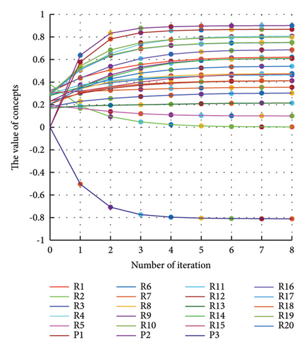
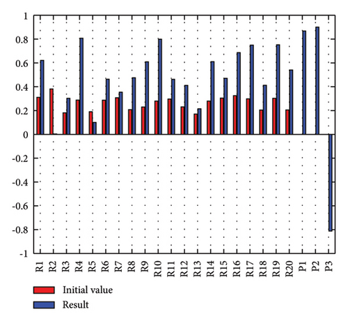
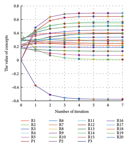
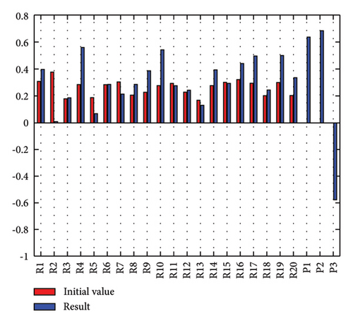
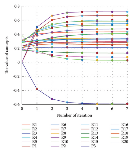
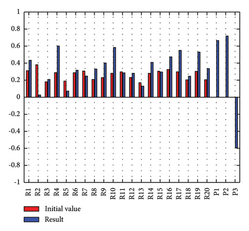
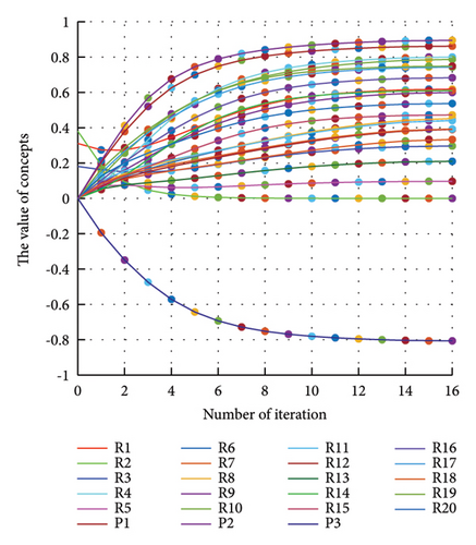
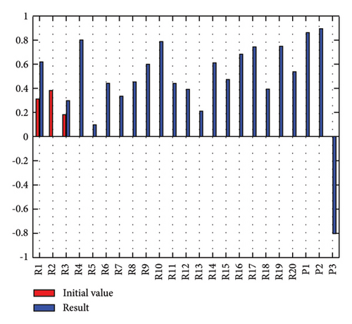
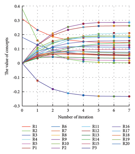
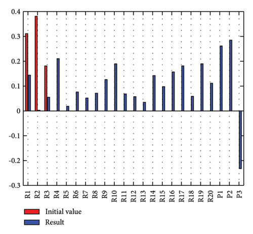
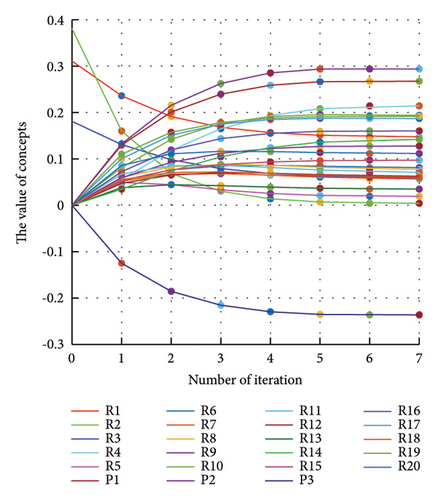
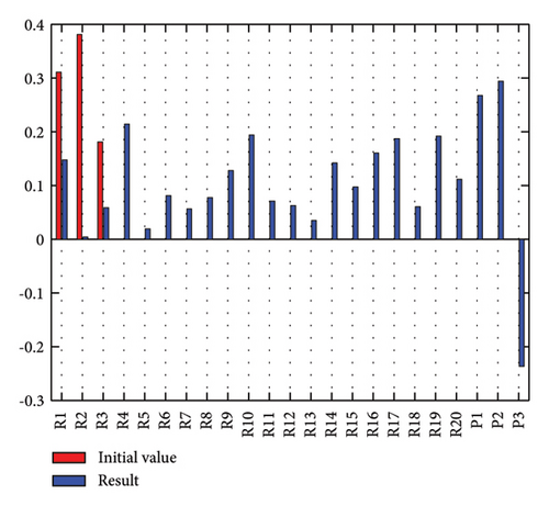
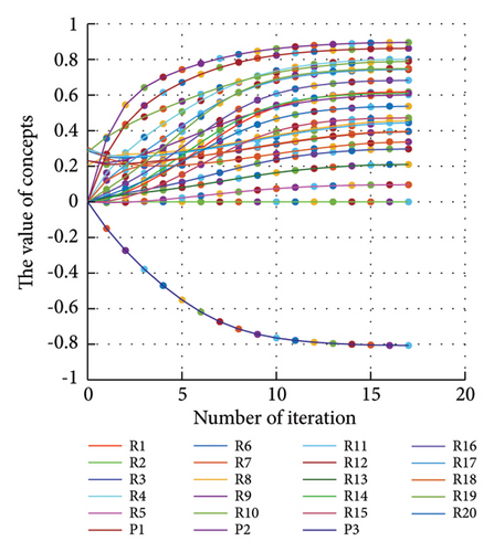
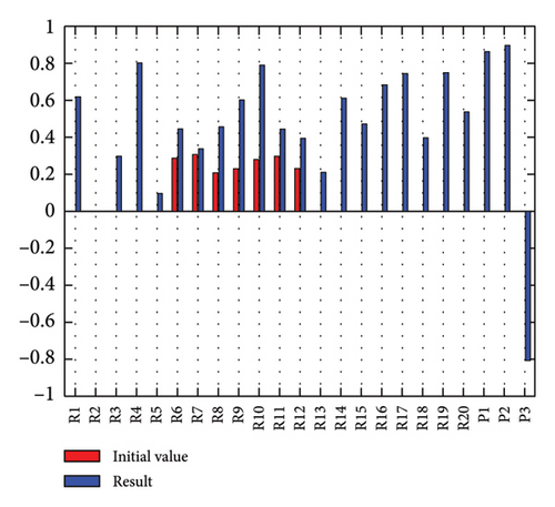
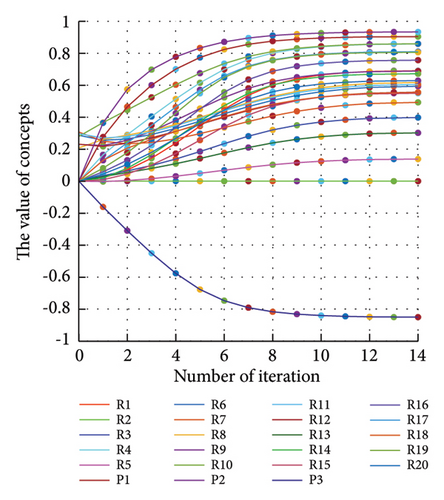
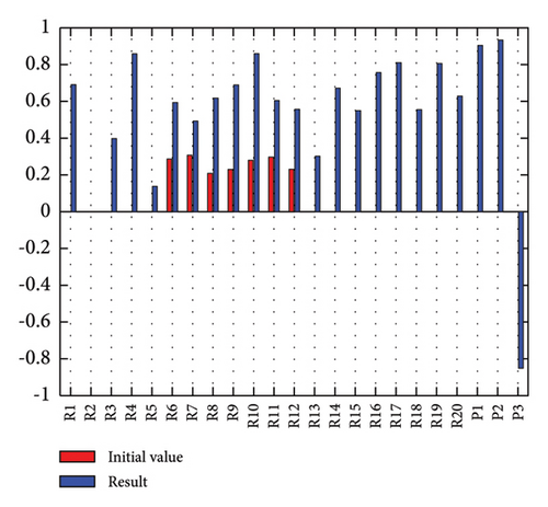
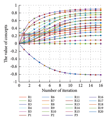
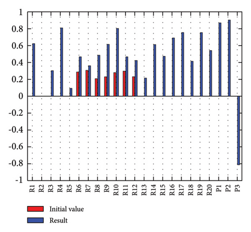
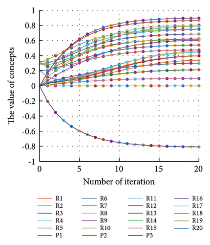
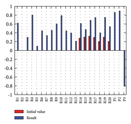
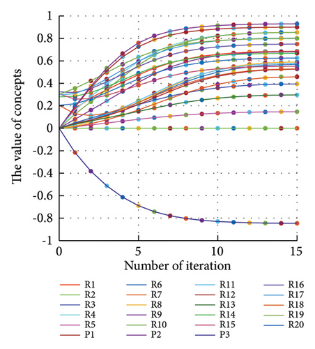
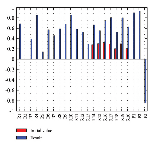
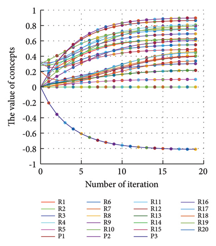
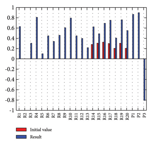
In addition to the numerical results presented in Table 4, the inference and the change of concepts during FCM iteration are presented for several scenarios in Figures 4–7 which are related to scenarios in which risks are activated as a group.
3.2.1. Scenario 1: Activation of All Risks in FCM
By activating all the risks of the model, the risk ranking differs from when the risks are considered statistically. Table 5 shows these differences.
| Rank | Considering the interdependency | Without considering interdependency |
|---|---|---|
| 1 | Defect in the domestic supply of essential raw materials | Sanction |
| 2 | Cash flow risk | Lack of good governance for medicines |
| 3 | Inefficient pricing policies | MOH conflicts of interest |
| 4 | Lobbying risks in the decision-making process | Dual exchange rate |
| 5 | Lack of good governance for medicines | Drug list limitation |
| 6 | MOH conflicts of interest | Lobbying risks in the decision-making process |
| 7 | Long cash collection cycle | Inefficient pricing policies |
| 8 | Pseudo-productivity (repacking) | Currency fluctuation |
| 9 | Inflation rate | Defect in the domestic supply of essential raw materials |
| 10 | Currency fluctuation | Money transfer problem |
| 11 | Money transfer problem | Cash flow risk |
| 12 | Change in legislation and policies | Pseudo-productivity (repacking) |
| 13 | Banking regulation instability | Interest rate |
| 14 | Interest rate | Long cash collection cycle |
| 15 | Dual exchange rate | Inflation rate |
| 16 | Drug list limitation | Change in legislation and policies |
| 17 | Political instability | Banking regulation instability |
| 18 | Demand fluctuations | Defect of international vision |
| 19 | Defect of international vision | Political instability |
| 20 | Sanction | Demand fluctuations |
Figure 4 illustrates the results of Scenario 1 and summarizes the FCM results trained by the NHL and AHL algorithms. By comparing Figures 4(a), 4(c), and 4(e), it can be observed that the trained FCM converges faster and this convergence is faster for the NHL than for the AHL.
3.2.2. Scenario 2: Activation of Macrorisks in FCM
In Scenario 2, supply and regulatory risks are more affected. In addition, costs have increased, time has increased, and quality has decreased. The model’s findings suggest that the SC of Iranian biopharmaceutical product makers, as part of the Iranian health system, is heavily influenced by Iran’s political situation, particularly at the time of the study. Figure 5 illustrates the outcomes of this scenario.
3.2.3. Scenario 5: Activation of Financial Risks in the FCM
Activation of financial risks leads to the activation of many risks in the model. Figure 6 illustrates that in this scenario, costs increase, time periods prolong, and quality decreases.
3.2.4. Scenario 7: Activation of Regulatory Risks in the FCM
The activation of regulatory risks leads to the activation of many model risks. According to Figure 7, the most affected risks are liquidity (0.854), poor supply of essential raw materials (0.853), conflicts of interest in the Ministry of Health (0.686), and long cash collection cycle (0.682). Similar to Scenario 2, in Scenario 7, costs have increased, the time has been prolonged, and quality has decreased (Figure 7).
4. Discussion
4.1. Impact of Risks on Cost, Time, and Quality
One of the most important outputs of the model is the calculation of the impact of risks on the three fundamental factors of the SC, namely, cost, time, and quality. This impact is presented in Table 6. If the influence of these three criteria is considered for risk importance and ranking, the priority of dealing with risks may shift. The ranking in Table 6 based on |P1| + |P2| + |P3| is from the highest value to the lowest value. The |⋅| symbol indicates the absolute value.
| Rank | Description | Time | Cost | Quality |
|---|---|---|---|---|
| 1 | Activating all risks | 0.869 | 0.890 | −0.923 |
| 2 | Activating macrorisks | 0.783 | 0.807 | −0.886 |
| 3 | Activating financial risks | 0.774 | 0.799 | −0.881 |
| 4 | Activating sanction risks | 0.769 | 0.795 | −0.874 |
| 5 | Activating regulatory risks | 0.753 | 0.761 | −0.871 |
| 6 | Activating political instability risks | 0.648 | 0.672 | −0.838 |
| 7 | Activating dual exchange rate risks | 0.644 | 0.681 | −0.833 |
| 8 | Activating money transfer problem risks | 0.652 | 0.686 | −0.815 |
| 9 | Activating currency fluctuation risks | 0.663 | 0.693 | −0.685 |
| 10 | Activating lack of good governance for medicine risks | 0.541 | 0.508 | −0.803 |
| 11 | Activating supply risks | 0.518 | 0.518 | −0.753 |
| 12 | Activating defect in the domestic supply of essential raw material risks | 0.518 | 0.518 | −0.753 |
| 13 | Activating long cash collection cycle risk | 0.465 | 0.465 | −0.699 |
| 14 | Activating MOH conflicts of interest risks | 0.710 | 0.000 | −0.867 |
| 15 | Activating inefficient pricing policy risk | 0.384 | 0.368 | −0.681 |
| 16 | Activating inflation rate risks | 0.000 | 0.416 | −0.667 |
| 17 | Activating demand risks | 0.485 | 0.485 | 0.000 |
| 18 | Activating demand fluctuation risks | 0.485 | 0.485 | 0.000 |
| 19 | Activating cash flow risks | 0.465 | 0.465 | 0.000 |
| 20 | Activating banking regulation instability risks | 0.409 | 0.425 | 0.000 |
| 21 | Activating organization and strategies’ risks | 0.000 | 0.000 | −0.799 |
| 22 | Activating defect of international vision riskss | 0.000 | 0.000 | −0.799 |
| 23 | Activating lobbying risks in the decision-making process risk | 0.000 | 0.000 | −0.716 |
| 24 | Activating interest rate risks | 0.000 | 0.573 | 0.000 |
| 25 | Activating change in legislation and policies’ risks | 0.515 | 0.000 | 0.000 |
| 26 | Activating pseudo-productivity (repacking) risks | 0.000 | 0.000 | 0.000 |
| 27 | Activating drug list limitation risks | 0.000 | 0.000 | 0.000 |
4.2. Performance Comparison Analysis
Fuzzy and FMEA represent distinct methods employed in risk assessment. In the context of FMEA, assessments delve into meticulous detail, categorizing potential failures within the system. Conversely, fuzzy methods adopt fuzzy approximation techniques to discern and classify failures [41]. Through the utilization of fuzzy rules, both systems and concerns are modeled, accounting for uncertainties and ambiguities inherent in the data. In the FMEA methodology, risks undergo evaluation and ranking based on criteria such as the probability of failure, severity of consequences, and detectability. Typically, this evaluation involves the assignment of scores, with subsequent interpretation based on the established criteria [26]. In contrast, fuzzy methods approach assessments through defuzzification and approximation, diverging from the scoring and interpretation framework utilized in FMEA. Fuzzy contrast techniques play a vital role in scrutinizing a set of values, utilizing fuzzy rules to adapt to imprecise and incomplete information. Both FMEA and the fuzzy method serve as tools for risk management. However, whereas FMEA places a stronger emphasis on quantitative- and quality-oriented evaluation, the fuzzy method has the capacity to integrate qualitative information and experiences [42]. Through the utilization of fuzzy elements and rules, the fuzzy method allows for a more elaborate modeling of risks, ambiguities, and interactions among various qualities [39]. This capability contributes to enhanced decision-making in the realm of risk management.
In contrast, opting for triangular membership functions in the fuzzy method (triangular FN (triFN)), as opposed to trapezoidal member functions (trapezoidal FN (traFN)) in FMEA, brings about a reduction in the volume of calculations. The triFN streamlines computations by minimizing complexity. Conversely, the adoption of traFN in the fuzzy method increases the number of adjustable parameters for uncertainty modeling, resulting in heightened complexity and an increased volume of calculations [43]. Both FMEA and the fuzzy method grapple with challenges inherent to fuzzy logic [44]. The implementation of the fuzzy method for risk modeling and evaluation necessitates intricate calculations, potentially leading to time-consuming and complex processes. Furthermore, dependence on expert opinions may present challenges, particularly in cases where there are divergent expert views on risk.
It is noteworthy that FCM and FMEA methods can complement each other, offering a comprehensive approach to risk management. The integration of these methods provides a robust framework for addressing various aspects of risk assessment and decision-making. The utilization of the FCM method-based FMEA, as discussed in this article, establishes a strong foundation for modeling uncertainties and ambiguities inherent in risks and processes. This approach not only integrates diverse and at times conflicting expert opinions but also stands out with its dynamic mode, allowing for agile adaptation to changes. The FCM method based on FMEA combines the strengths of both the fuzzy method and FMEA while avoiding the drawbacks associated with the conventional fuzzy method. A notable advantage of the FCM method based on FMEA lies in its ability to model intricate combinations of risks using fuzzy rules and integrating diverse criteria. This proves invaluable in addressing the multicriteria and complex nature of certain risks. Moreover, its adaptability to changes and developments over time makes it well-suited for dynamic and complex risk management scenarios. Being rooted in fuzzy logic theory, the FCM method exhibits flexibility in modeling [34, 36]. Fuzzy rules can be finely tuned to adjust weightings and relationships between factors based on varying conditions and inputs, facilitating seamless adaptation of the model to different system states. Another noteworthy strength of the FCM method based on FMEA is its versatility, being applicable to training both with and without a supervisor [38].
The implementation of sensitivity analysis provides a quantitative means of comparing different methods. To ensure the resilience of our model, a systematic approach is undertaken. Initial values of activated risks are increased by 20%, followed by running the model. Subsequently, these values are decreased by 20%, and the model is rerun. This meticulous process is replicated for the FMEA method, the fuzzy method with triFNs based on FMEA, and the fuzzy method with traFNs based on FMEA. The graphical representation of these results is presented in Figure 8.
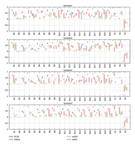
Upon meticulous examination of Figure 8, it is evident that the FCM method based on FMEA exhibits a more stable response, with less pronounced changes compared to other methods. This observation underscores the heightened robustness of the FCM method based on FMEA when subjected to variations in the initial values of activated risks.
Advantages of employing NHL and AHL algorithms in phase III for training the FCM are as follows:
- (a)
NHL empowers the FCM to depict nonlinear cause-effect associations, commonly encountered in practical supply chain dynamics, resulting in more precise system representations and enhanced predictive abilities
- (b)
AHL facilitates the FCM to dynamically adjust its internal weights and structure based on fresh data and feedback, thereby rendering the model more adaptable and responsive to alterations in the supply chain milieu
Enhanced convergence speed and training efficiency: Studies have demonstrated that the NHL and AHL algorithms converge at a faster rate compared to conventional FCM training methodologies, such as the standard Hebbian learning approach. This accelerated convergence facilitates more efficient training of the FCM model, enabling rapid updates and iterations to enhance the precision of risk analysis.
Enhanced scenario analysis and sensitivity testing: The flexibility and adaptability provided by NHL and AHL algorithms can enable more robust scenario analysis and sensitivity testing of the FCM. This is crucial for evaluating the impacts of different risk factors and assessing the resilience of the supply chain under various conditions.
Potential limitations and challenges in implementing the FCM-based approach are cited as follows:
Data availability and quality: The FCM-based methodology heavily depends on thorough and precise data concerning supply chain risks, their causal interconnections, and the related parameters. Acquiring such data may pose challenges within the Iranian biopharmaceutical sector, where data collection and sharing practices might not be as advanced. Potential mitigation: Establish close collaborations with industry stakeholders to enhance data collection and sharing mechanisms. Leverage expert knowledge and employ methodologies such as fuzzy set theory to handle incomplete or uncertain data effectively.
Model complexity and development effort: Building and validating a sophisticated FCM that precisely mirrors the biopharmaceutical supply chain can be a challenging and time-intensive endeavor. The incorporation of advanced algorithms such as NHL and AHL could potentially elevate the complexity of the modeling process. Potential mitigation: We implement semiautomated or knowledge-driven strategies to streamline the FCM development process. In addition, leverage modular design principles and existing domain expertise to enhance the model’s efficiency.
Organizational adoption and change management: Introducing an innovative, data-centric risk analysis approach such as the FCM-based method might encounter opposition from conventional risk management practices prevalent in Iranian pharmaceutical firms. Securing approval and support from stakeholders may necessitate substantial change management endeavors. Potential mitigation: We engage industry leaders and key decision-makers at an early stage and offer thorough training and documentation to showcase the advantages of adopting an FCM-based approach.
5. Conclusion
This paper presents a dynamic risk assessment of the Iranian biopharmaceutical supply chain (SC), which was not taken into account in earlier studies on Iranian pharmaceutical SC. The results show that the SC of biopharmaceutical and chemical drugs was not significantly different, but the impact and importance of risks in the SC can differ. During the study period, the political situation in Iran had an impact on biopharmaceutical companies and the drug SC as an essential aspect of the healthcare system. This study examined the risks that have the most significant impact on the SC of Iranian biopharmaceutical manufacturers. Analysis and modeling of SC risks of companies producing biopharmaceuticals were also presented. Given the limitations of existing risk analysis tools to accurately predict the behavior of risks and analyze them dynamically, a fuzzy cognitive map (FCM) was used. Various situations were created to investigate and acquire FCM inference; hence, the FCM was trained using the nonlinear Hebbian learning and active Hebbian learning algorithms. Finally, the results of inference, FCM simulation, and analysis were presented.
Employing FCMs, this study offers crucial insights for anticipating failure effects and causes in intricate systems. Accounting for interdependence among risk factors and consequences enhances the accuracy of risk analysis, aiding decision-makers. This approach provides robust support for managers to identify critical failures and implement effective mitigation strategies, thereby enhancing overall risk management. Furthermore, the integration of cutting-edge technologies such as edge cloud computing and deep learning underscores the synergistic capacity of amalgamating computational prowess with domain proficiency to amplify risk evaluation capabilities [45–47]. Through harnessing the distributed computational potency and swift data processing attributes of edge cloud computing, in conjunction with the feature extraction and pattern recognition proficiencies of deep learning algorithms, risk appraisal models can attain heightened sophistication and subtlety, culminating in more precise and dependable outcomes. However, the FCM method based on FMEA, while potent, is not without its limitations. Notably, it involves a higher volume of calculations compared to FMEA, posing potential challenges related to computational efficiency and time constraints. A critical consideration lies in the reliance on expert opinions to shape the structure of FCM, encompassing concepts, graph nodes, and their interrelationships. Any errors during the initial stages of risk identification, expert interviews, or risk screening may compromise the accuracy and reliability of subsequent results generated by the FCM method.
To enhance the practical applicability of the FCM method based on FMEA, it is crucial to recognize and address these limitations. Implementing rigorous validation processes, continually refining input data, and maintaining an iterative dialogue with domain experts are proactive measures that can mitigate these challenges and strengthen the overall robustness of the methodology.
Ethical Approval
The study was confirmed by the Ethics Committee of Tehran University of Medical Sciences (TUMS): IR.TUMS. VCR.REC.1397.675.
Disclosure
This study was part of Hadi Abbasian PhD thesis registered in Tehran University of Medical Sciences [48].
Conflicts of Interest
The authors declare that there are no conflicts of interest.
Open Research
Data Availability
Data used to support the findings of this study are available in supplementary information files. More data will be available on request.


