Numerical Investigation of Ternary Hybrid Non-Newtonian Nanofluids and Heat Transport Over an Inclined Shrinking Sheet Utilizing Artificial Neural Network
Abstract
The purpose of the study is to investigate the thermal proficiency of a trihybrid magnetized water-based cross nanofluid over an inclined shrinking sheet. Cross-fluid is the best model to investigate the fluid flow at a very high and very low share rate. There are three nanoparticles that are added in based fluid (water) to form the requisite posited ternary hybrid nanofluid. Moreover, heat transport analysis is scrutinized by incorporating the melting conditions. The obtained nonlinear system of partial differential equations (PDEs) from assumed physical assumption is converted into the nonlinear setup of ordinary differential equations (ODEs). These ODEs are passed under the boundary value problem of a fourth-order (bvp4c) MATLAB program for numerical results. With the help of bvp4c, data are further trained through an artificial neural network and results are predicted. Results are compared with both techniques and found smooth agreement. The obtained numerical results provide valuable insight for optimizing heat transfer processes involving nanoparticle-enhanced fluid on inclined shrinking sheets. From the results, it is concluded that the inclusion of nanoparticles enhances the viscosity and thermal conductivity of the fluid. High temperatures make rapid heat transfer scenarios.
1. Introduction
The significance of incorporating three nanoparticles in base fluid over the inclined stretching sheet is paramount in enhancing the accuracy and efficiency of heat transfer applications. Ternary hybrid nanofluids are composed of three solid nanosized nanoparticles. Ternary hybrid nanofluid can augment the heat transport, rheological properties, and thermal conductivity in fluid flow dynamics. Moreover, ternary hybrid nanofluids on an inclined stretching sheet provide valuable insights for real-world applications, such as in thermal management systems, and industrial processes and contributing to advancements in energy efficiency and this research can optimize nanofluid applications in various industries. Barman, Roy, and Chamkha [1] used special properties in the water to measure temperature changes and understand how entropy is created. Alzu’bi et al. [2] conducted comprehensive research on Williamson’s hybrid nanofluid and made a numerical attempt through a magnetized fluid containing tiny particles. Ali et al. [3] discussed the effects of entropy production or generation during the heat transfer process in a carboxymethyl cellulose water-based cross-hybrid nanofluid. A new model has been developed by Berrehai, Dinarvand, and Khan [4] to study the flow of a wedge that is moving and warmed by convection. The model focuses on the generation of entropy and uses a hybrid combination of mass and nanofluid. Ahmed et al. [5] investigated the heat transfer in a water fluid containing tiny graphite particles through convection, using electricity and magnetism to control the movement of the nanofluid. A study was conducted by Wahid et al. [6] through electromagnetic waves to investigate the effect of thermal radiation on the flow of a nanofluid over a permeable flat plate.
The cross model holds substantial significance in fluid dynamics. This model is a mathematical representation to investigate the fluid behavior, and all phenomena occurring within fluids. Its viscosity model can explain the characteristics of fluid at very high and very low shear rates. This capability makes this model unique from other ones. Many studies related to cross-fluid like Ayub et al. [7] investigated the transfer of heat in blood over some time, utilizing the cross nanofluid model along with the Keller–Box and boundary value problem of a fourth-order (bvp4c) solver technique. Understanding the relevance of bioconvection analysis for cross nanofluid flow involving microorganisms and its correlation with heat and rotation is described by Anjum et al. [8]. In this paper, the author studied the significance of this phenomenon in the movement of nanofluids containing microorganisms. The phenomenon of bioconvection, around a cylinder with a cross-fluid model attached to activation energy and characteristics of second-order slip are explored by Aljaloud, Manai, and Tlili [9]. The viscosity behavior of the cross nanofluid about the presence of a magnetic force over a thin stretching sheet in two different directions is discussed by Darvesh et al. [10]. Moreover, Ayub et al. [11] discussed the effects of different types of forces having different magnetic properties on a cross-fluid flowing over two rotating disks to manipulate the fluid flow consequences. Khan et al. [12] presented a numerical analysis of a cross nanofluid in the context of radiative stagnation point flow due to a shrinking surface.
Thermal science is facing a lot of problems like air pollution, environmental degradation, economic burden, increased greenhouse gas emissions, energy inefficiency, socioeconomic disparities, and energy waste, resource depletion due to the consumption of heat. In fluids, the consumption of heat can only be increased by improving the thermal conductivity of that fluid. Thermal conductivity is vital for ensuring efficient and effective heat transfer, improving energy efficiency, enhancing thermal management, and optimizing the performance of various heat-related applications and systems. The incorporation of ternary hybrid nanoparticles into fluids can enhance thermal conductivity, customizable thermal properties, and improve heat dissipation. Anjum et al. [13] presented a study to analyze the heat transfer capabilities of Sutterby nanoliquid during its melting process. Zeeshan et al. [14] used a flat channel to investigate the errors and stability of nanofluid. The study revealed that the fluid can transfer heat and mass and its ability to conduct heat changes uniquely. Later, Darvesh et al. [15] conducted a study on the flow of a type of fluid that contains tiny particles and microorganisms in motion around a three-dimensional cylinder by using cross-fluid viscosity model at very high shear rates. The base fluid containing sodium alginate (NaC6H7O6) over a three-dimensional rotating frame was examined by Ali et al. [16] under different thermal attributes. Khan et al. [17] studied thermally dissipative micropolar hybrid nanofluid in the context of gyrotactic microorganisms over a spinning needle influenced by Hall current effects.
Inclined sheet geometry has a significant role in enhancing heat transport in nanofluids. The inclination angle affects the flow dynamics, which in turn influences the thermal boundary layer, heat transfer rates, and overall fluid behavior. The inclination enhances the convection currents and augments the heat transfer rate, which is crucial in applications, such as cooling systems, thermal management in electronics, and chemical processing. Consequently, the study of heat transport in nanofluids over inclined surfaces is essential for optimizing the design of thermal systems that require precise control over heat dissipation. Several studies have investigated the influence of inclined sheet geometry on the heat and mass transfer characteristics of various nanofluids, focusing on different models and physical effects. Isa et al. [18] explored the Soret–Dufour effects in a three-dimensional magnetohydrodynamics (MHD) Newtonian fluid flow over an inclined plane. Their findings revealed that the inclination of the sheet affects the fluid’s thermal and concentration boundary layers. In another study, Isa et al. [19] examined the heat and mass transfer over an inclined sheet. Parvin et al. [20] focused on the magnetized Maxwell nanofluid flow over a shrinking inclined surface. Their study emphasized the impact of sheet inclination on the thermal and mass transport properties. Furthermore, Mohd et al. [21] investigated the thermal properties of a water-based hybrid nanofluid (Cu─Al2O3) flowing over an inclined plane. These studies collectively underscore the importance of inclined sheet geometry in enhancing heat and mass transfer in nanofluids.
1.1. Motivation
In the pursuit of scientific excellence, the thermal proficiency of trihybrid magnetized water-based cross nanofluid over an inclined shrinking sheet represents a key exploration of fluid dynamics and nanoscience in the existing examination. Utilization of artificial neural networks (ANNs) and the bvp4c solver, this study presents the best numerical solution to an assumed physical problem.
1.2. Novelty
- •
Exploration of the use of the cross-fluid model with very high and very low shear rate viscosity.
- •
Investigation of the thermal proficiency of a trihybrid magnetized water-based nanofluid.
- •
To provide a basis for optimizing processes involving nanoparticle-enhanced fluid on inclined shrinking sheets.
- •
Scrutiny of heat transport analysis by heat flux model.
- •
To obtain the mathematical solution of the obtained nonlinear system of partial differential equations (PDEs).
- •
To apply the ANN and bvp4c MATLAB program for numerical results.
1.3. Organization of Paper
Further, this paper is organized as follows: Section 2 explains the physical formulation of the problem, and Section 3 is related to mathematical design. Section 4 presents the bvp4c numerical structure, Section 5 expresses the validity of the study, and Sections 6 and 7 are established for the ANN technique and its formulation. Section 8 reveals the analysis of the results, and Section 9 explains the key conclusion of the study and shows the future direction of the work.
2. Description of the Problem
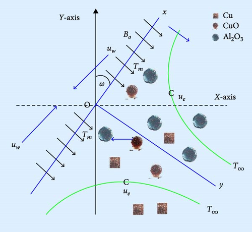
Let us consider that a shrinking inclined sheet moving with velocity uw(x), and the velocity of the inviscid fluid or ambient fluid is ue(x). The flow is incompressible, two-dimensional, laminar, and steady. The configuration of the flow mechanism is shown in Figure 1, where the numerical investigation of the ternary hybrid non-Newtonian nanofluids and heat transport over an inclined shrinking sheet along with melting effects. In addition, the impact of the Cattaneo–Christov heat flux, mixed convection, and magnetic field are also included. Also, three nanoparticles, copper oxide (CuO), copper (Cu), and aluminum oxide (Al2O3), are included to enhance the thermal conductivity of the fluid. Free stream temperature is denoted by T∞ and melting temperature is denoted by Tm.
2.1. Application of the Geometry
Inclined shrinking sheet has critical and diverse applications across various industries and technologies. In the textile industry, these geometries facilitate uniform dyeing and drying of fabrics. Aerospace engineering employs inclined shrinking sheets to optimize heat transfer, and fluid flow for improved thermal protection systems and model aerodynamic surfaces. In polymer science, they are essential in stretching processes. The thin film coating industry utilizes these geometries to achieve uniform coating and optimal thermal management in the production of solar cells, optics, and electronics. In cooling systems, inclined shrinking sheets are used for thermal efficiency. Finally, biomedical devices, such as prosthetics and artificial organs, utilize inclined shrinking sheets to ensure precise control over fluid dynamics and heat transfer.
3. Mathematical Background of the Model
The thermophysical properties of nanomaterials (Cu, CuO, and Al2O3) [23] included in the existing study and complete mathematical forms of each nanoparticle are described through Tables 1 and 2 while the experimental data of the thermophysical properties are mentioned in Table 3. The single-phase model consists of only one phase with averaged properties. This model’s primary advantage is its simplicity. The single-phase model is particularly useful in scenarios where the interfacial effects between phases are negligible. However, this simplification also brings significant disadvantages. It overlooks the interactions between different phases, such as mass transfer, phase change, and interfacial forces, leading to less accurate predictions in systems where these interactions are crucial.
| Name of properties | Correlation |
|---|---|
| Thermal diffusivity | |
| Viscosity | |
| Heat capacity | |
| Density | |
| Thermal expansion | |
| Thermal conductivity | |
| Electrical conductivity | |
| Properties | Correlation |
|---|---|
| Thermal diffusivity | |
| Viscosity | |
| Heat capacity | |
| Density | |
| Thermal expansion | |
| Thermal conductivity | |
| Electrical conductivity | |
| Properties | Water | CuO | Cu | Al2O3 |
|---|---|---|---|---|
| ρ | 997.1 | 6320 | 8933 | 3970 |
| CP | 4179 | 531.8 | 385 | 765 |
| k | 0.613 | 76.5 | 401 | 40 |
| σ | 5.5 × 10⁻⁶ | 6.9 × 10⁻² | 59.6 × 10⁶ | 35 × 106 |
| βT | 21 | 1.80 | 1.67 | 0.85 |
| Pr | 6.2 | — | — | — |
These three nanoparticles CuO, Cu, and Al2O3 present unique properties when dispersed in fluids and they possess both advantages and disadvantages. The CuO nanoparticles enhance thermal conductivity and are suitable for cooling systems and medical applications. Cu nanoparticles improve thermal and electrical conductivity, which is beneficial for electronic cooling and heat exchangers. On the other side, they can be prone to oxidation, leading to performance degradation over time. Al2O3 nanoparticles are excellent for thermal stability and mechanical strength and, on other hand, Al2O3 nanoparticles may have lower thermal conductivity enhancement compared to metallic nanoparticles.
4. Validity of the Code
The process of verification of the code has produced good results for f″(0) and − θ′(0). Tables 4 and 5 are evidence for this smooth agreement. The validation process not only ensures the fidelity of our codebase but also substantiates its adherence to the best practices and theoretical foundations elucidated in the broader academic context.
| Me | f″(0) | |||
|---|---|---|---|---|
| Bachok, Ishak, and Pop [27] | Wahid et al. [28] | Current work | ||
| — | — | bvp4c | ANN outcome | |
| 0 | −1.887 | −1.887 | −1.87693456 | −1.8889876 |
| 1 | −1.580 | −1.580 | −1.59804976 | −1.5898765 |
| 2 | −1.442 | −1.442 | −1.47827654 | −1.4476098 |
| 3 | −1.359 | −1.359 | −1.35765671 | −1.3698879 |
- Abbreviation: ANN, artificial neural network.
5. Methodology
6. ANN Procedure
- 1.
Neurons: These are fundamental units of this robust scheme. Each selected neuron receives one or more inputs from data.
- 2.
Weights: Weights describe the connections between neurons.
- 3.
Activation function: This function calculates the output of a neuron.
- 4.
Layers: Structure of ANN is based on layers. Simulations are taken place layer by layer.
- 5.
Feedforward process: Here input data are passed through the network to generate an output. This process starts with the input layer, where each neuron receives the initial data. The data are then processed and passed to the subsequent hidden layers through weighted connections.
- 6.
Training: Training in neural networks constitutes an iterative process whereby the model autonomously refines its internal parameters through exposure to voluminous and often multifaceted datasets.
- 7.
Loss function: It epitomizes a quintessential mathematical construct that quantifies the divergence between the network’s predicted outputs and the actual target values. The landscape of the loss function, often characterized by its intricate topology replete with local minima and saddle points, profoundly influences the efficacy of the gradient descent-based optimization processes.
- 8.
Backpropagation: This process commences with a forward pass, wherein input data propagate through the network’s layers, yielding an output. The ensuing phase involves the backward propagation of the computed error, emanating from the output layer and traversing backward through the hidden layers. This reverse traversal is facilitated by the application of the chain rule, allowing for the systematic calculation of gradient vectors corresponding to each weight.
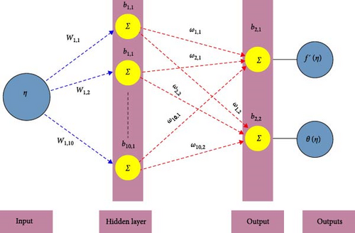
Additionally, the current study’s hidden layer, output layer, weight and bias mechanisms, along with the required training setup, are illustrated in Figures 2 and 3, respectively. Figure 2 depicts a network with a single input layer vector, featuring 10 neurons in the hidden layer, and two output neurons. Meanwhile, Figure 3 presents an architecture with one hidden layer, one output layer, and 10 neurons for training the ANN.

7. Formulation of ANN Scheme and Parameter Fixation
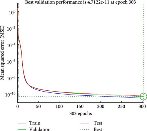
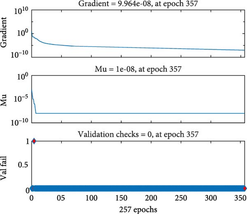
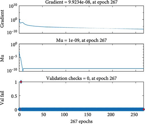
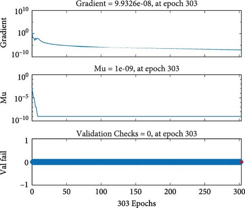
In this section, the formulation of the ANN and parameter fixation is investigated. Comprehensive exploration of data training process, we considered three distinct scenarios, and each scenario is related with distinct parameters. Scenario 1 deals with the cross-fluid index parameter. This parameter is a pivotal factor in our study because this mathematical model generates PDEs for the current physical problem. Its values are systematically varied with 0.3, 0.6, and 0.9. In scenario 2, we scrutinized the impact of the Hartmann parameter by introducing the variations of 0.1, 0.2, and 0.3. The last scenario deals with thermal relaxation parameter scrutiny with variations at 0.001, 0.002, and 0.003. Through this analysis training sessions, fitness graph evaluations, regression analyses, and error plot assessments, our findings unequivocally demonstrate that the data were adeptly trained optimally for each specific case. The results indicate a robust adaptability to varying parameter configurations, reinforcing the efficiency and effectiveness of our data training approach across diverse scenarios. In addition, Table 6 shows complete details of the formulation of the ANN scheme, parameter fixation, performance, gradient, mu, and period for each case.
| Parameter | Value | Case | Performance | Gradient | Mu | Epoch | Time (s) | |||
|---|---|---|---|---|---|---|---|---|---|---|
| Initial value | Stopped value | Initial value | Stopped value | Initial value | Stopped value | |||||
| n | 0.3 | i | 4.35 | 2.44e-10 | 6.01 | 9.96e-08 | 0.001 | 1e-08 | 357 | 1 |
| 0.6 | ii | 4.55 | 4.28e-10 | 5.76 | 9.97e-08 | 0.001 | 1e-08 | 285 | 1 | |
| 0.9 | iii | 1.23 | 3.23e-11 | 2.45 | 9.91e-08 | 0.001 | 1e-09 | 259 | 1 | |
| Mn | 0.1 | i | 3.05 | 2.55e-11 | 4.28 | 9.92e-08 | 0.001 | 1e-09 | 267 | 1 |
| 0.2 | ii | 2.36 | 3.29e-10 | 3.85 | 9.96e-08 | 0.001 | 1e-08 | 297 | 3 | |
| 0.3 | iii | 2.82 | 7.74e-10 | 5.25 | 9.94e-08 | 0.001 | 1e-08 | 291 | 1 | |
| δT | 0.001 | i | 2.59 | 3.07e-11 | 4.13 | 9.93e-08 | 0.001 | 1e-09 | 303 | 1 |
| 0.002 | ii | 2.5 | 7.52e-10 | 3.72 | 9.94e-08 | 0.001 | 1e-08 | 267 | 2 | |
| 0.003 | iii | 2.18 | 3.99e-10 | 3.16 | 9.96e-08 | 0.001 | 1e-08 | 292 | 2 | |
- Abbreviation: ANN, artificial neural network.
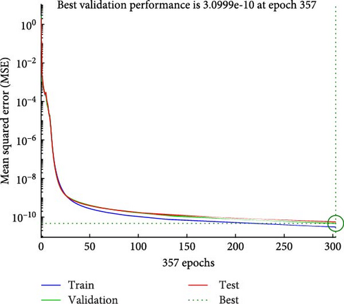
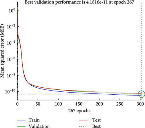
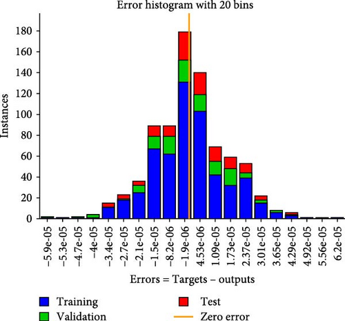
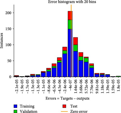
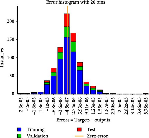
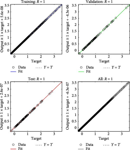
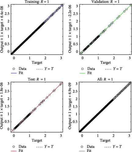
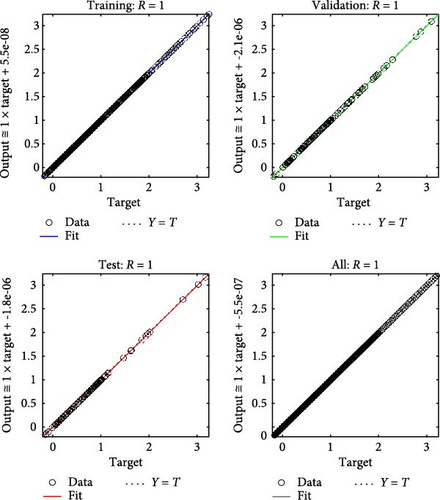
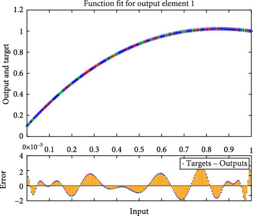
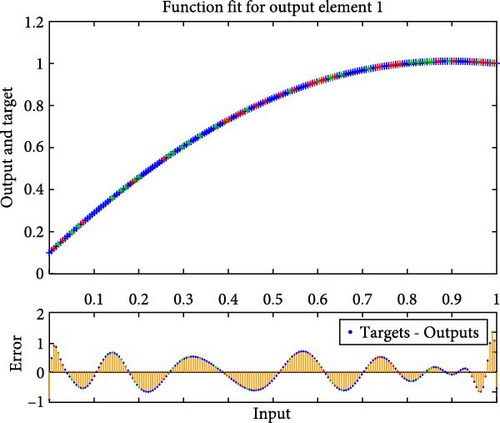
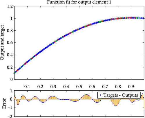
Figures 4a–c–8a–c are placed and these figures show that during the training we got the best validation performance, gradient, mu, and validation checks estimation, error histogram, regression analysis, and fitness graphs for output with a variation of cross-fluid index (0.3, 0.6, 0.9), Hartmann number (0.1, 0.2, 0.3), and thermal relaxation parameter (0.001, 0.002, 0.003), respectively. The best numerical value for performance is found at 3.0999e-09 at 357 epochs, 4.1816e-11 at 267 epochs, and 4.7122e-11 at 303 epochs for cross-fluid index, Hartmann parameter and thermal relaxation parameter are shown in Figure 4a–c, respectively. Figure 5a–c shows the numerical output values of gradient, mu, and validation checks estimation during ANN training for variation physical parameters. This figure shows that validation checks are zero for each case and numerical values of mu are 1e-08, 1e-09, and 1e-09 for each case, and 9.96e-08, 9.9234e-08, and 9.9326e-08 are the numerical values of gradient function. Figure 6a–c represents the related error histogram. The error histogram is divided into 20 bins and the best errors are calculated as −1.9e-06, 4e-07, and −4.5e-0.7. Figure 7a–c describes regression analysis during training, validation, test, and overall. In all cases, regression is 1 which shows that training is best and linear. Figure 8a–c describes the error plots in different situations.
8. Results and Discussion
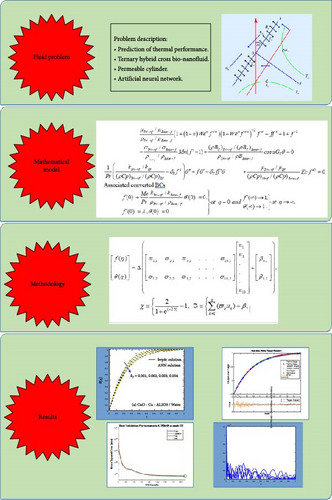
In this section, the discussion about the impact of several parameters on velocity and temperature profile, numerical outcomes of physical problems by ANN and bvp4c, and error plots of both techniques are made comprehensively. There are several physical parameters involved in the current study like Weissenberg’s number (We), cross-fluid index (n), Hartmann parameter(Mn), melting parameter (Me), stretching/shrinking parameter (λ), local Grashof temperature number (GT), the volume fraction of CuO, the volume fraction of Cu, the volume fraction of Al2O3, and thermal relaxation parameter (δT). Variations of three parameters cross-fluid index, Hartmann parameter, and thermal relaxation parameter are processed with ANN. All ANN graphs like training sessions, fitness graph evaluations, regression analyses, and error plot assessments are established and for further parameters, geometrical interpretation is shown through bvp4c, and ANN figures and estimation of error plots are also sketched. Figure 9 shows the overall pictorial representation of the current study.
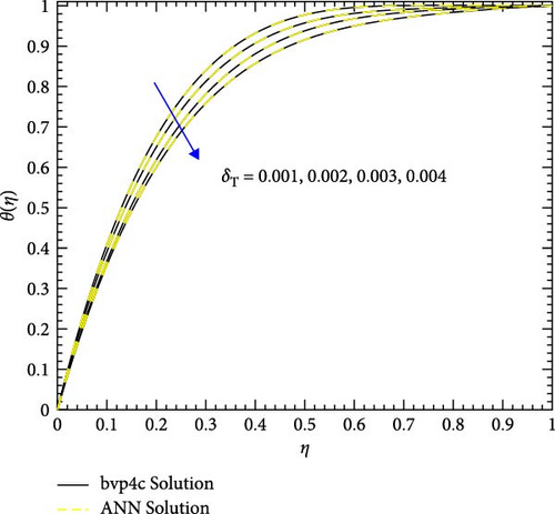
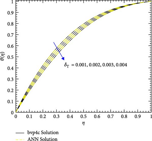
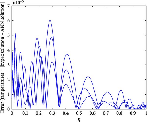
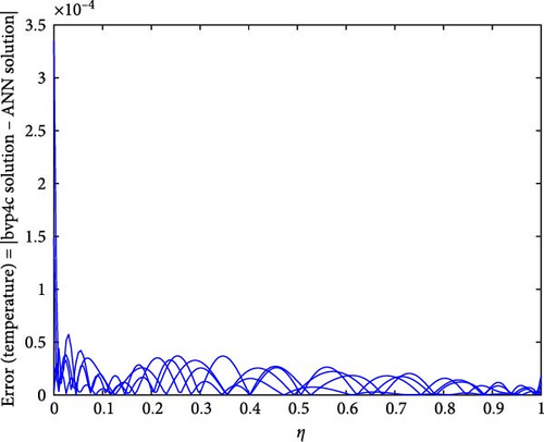
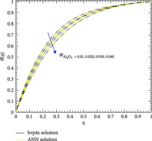
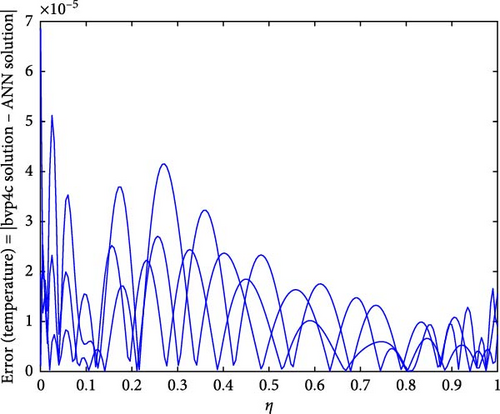
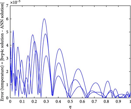
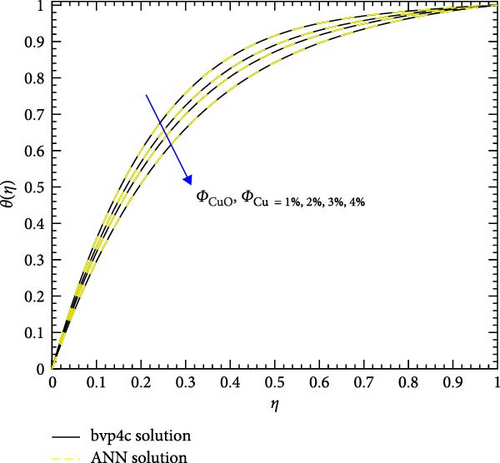
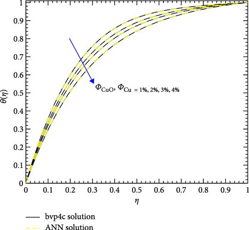
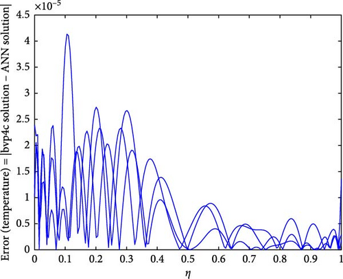
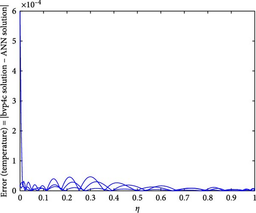
Figures 10a,b–29a,b are plotted for geometrical interpretation of physical parameters on f′(η) and θ(η) for both cases of trihybrid ([CuO − Cu − Al2O3]/H2O) and hybrid ([CuO − Cu]/H2O) nanofluid with ANN/bvp4c scheme. Each figure is plotted with the help of ANN and bvp4c methods, which gave smooth agreement and impact of each physical parameter is seen on trihybrid and hybrid nanofluid. Further error plots are there which show the error analysis between both numerical schemes. Figure 10a,b shows the impact of local Grashof temperature number on velocity of trihybrid and hybrid cross nanofluid flow and Figure 11a,b shows error estimation between ANN and bvp4c. The decrement in the velocity of fluid is found with numerical growth in the magnitude of local Grashof temperature number. This number relates with buoyancy-induced flow within a fluid adjacent to a heated or cooled surface. Local thermal properties are significantly altered due to the presence of nanoparticles, and they enhance thermal conductivity. So, by increasing this number, a decrease is seen in the overall fluid velocity.
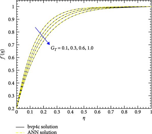
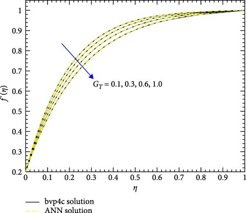
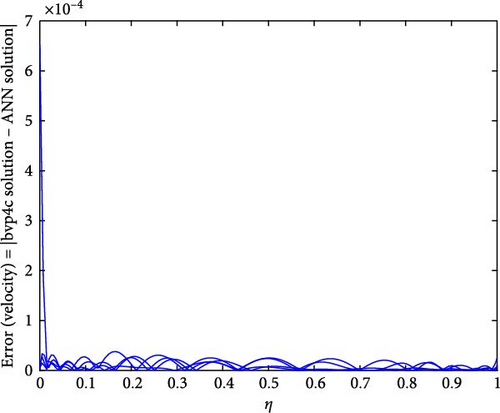
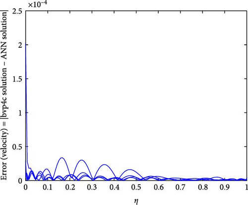
Figure 12a,b shows the impact of stretching/shrinking parameters on the velocity of trihybrid and hybrid cross nanofluid flow, and Figure 13a,b shows error estimation between ANN and bvp4c. With the augmentation of the stretching/shrinking parameter, the velocity of fluid in the presence of nanoparticles increases. This parameter gives an indication of the deformation of sheets. As the stretching/shrinking parameter increases, the sheet undergoes deformation, and this leads to changes in BCs and its surface area. The presence of nanoparticles also influences the viscosity of the fluid, reducing internal friction and facilitating smoother flow hence velocity increases. Figure 14a,b shows the impact of the melting parameter on the velocity of trihybrid and hybrid cross nanofluid flow, and Figure 15a,b shows error estimation between ANN and bvp4c. The velocity of fluid decreases with increasing values of the melting parameter in the presence of nanoparticles. This parameter is associated with the melting point of the nanoparticles and influences their thermal properties. Whenever this parameter increases, the nanoparticles tend to exhibit higher melting points, and this leads to enhanced thermal stability and hence temperature decreases. Figure 16a,b shows the impact of the Hartmann parameter on the velocity of trihybrid and hybrid cross nanofluid flow, and Figure 17a,b shows error estimation between ANN and bvp4c. The Hartmann number explains the interaction between magnetic fields and electrically conductive fluids. According to the present cross nanofluid flow with the presence of Cu, CuO, and Al2O3 nanoparticles, an increase in the Hartmann parameter tends to decrease the velocity of the fluid. This increased parameter produces magnetic field strength. This magnetic field exerts a drag force on the conductive fluid containing the suspended nanoparticles and hence hindrance is felt by fluid layers and due to this overall fluid velocity decreases. Furthermore, the combined effects of the magnetic field and nanoparticle presence contribute to a decrease in fluid velocity as the Hartmann parameter increases. Figure 18a,b shows the impact of cross-fluid index parameter on the velocity of trihybrid and hybrid cross nanofluid flow, and Figure 19a,b shows error estimation between ANN and bvp4c. The decrement in fluid velocity is seen with increasing values of the cross-fluid index parameter in the presence of Cu, CuO, and Al2O3 nanoparticles. Increment in this parameter creates dominance of viscous forces which leads to a decrease in fluid velocity. The presence of nanoparticles also helps in enhancing the viscosity of the fluid and resistance to flow, hence fluid velocity decreases. Figure 20a,b shows the impact of Weissenberg number on the velocity of trihybrid and hybrid cross nanofluid flow, and Figure 21a,b shows error estimation between ANN and bvp4c. The velocity of a fluid is observed to decrease with an increase in the Weissenberg number when nanoparticles such as Cu, CuO, and Al2O3 are introduced. This is because of enhanced viscoelastic properties, and these are induced by the presence of nanoparticles (Cu, CuO, and Al2O3). Weissenberg number is the ratio of elastic forces to viscous forces, and this becomes more pronounced and signifies a dominance of elastic behavior. These nanoparticles cause increased elasticity and viscoelastic networks in the fluid. This fact leads to a greater resistance to deformation and a subsequent reduction in fluid velocity.
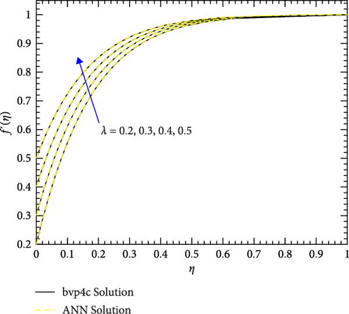
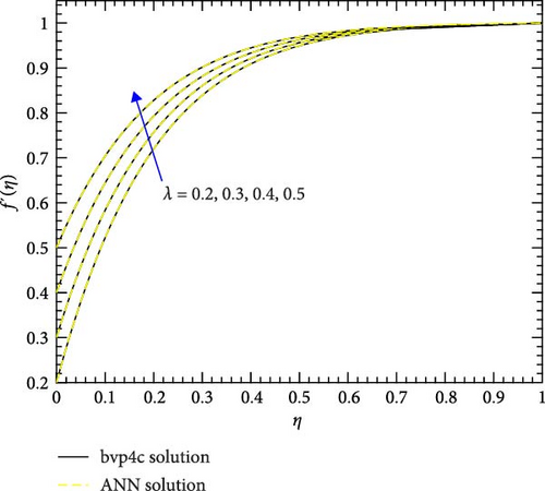
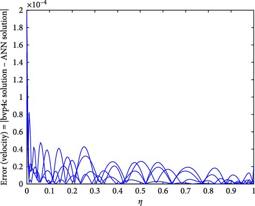
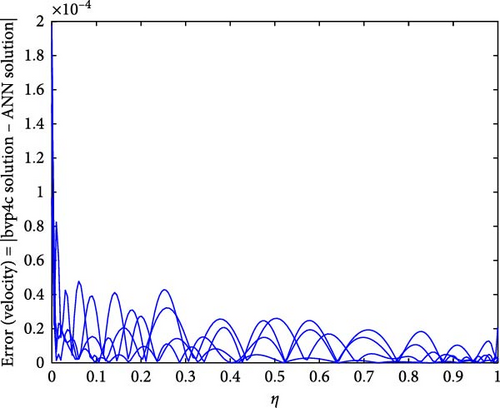
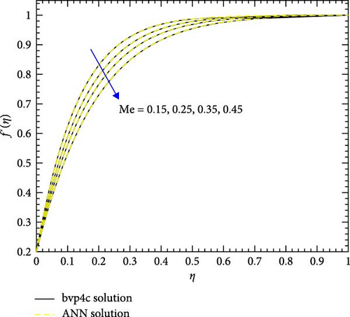

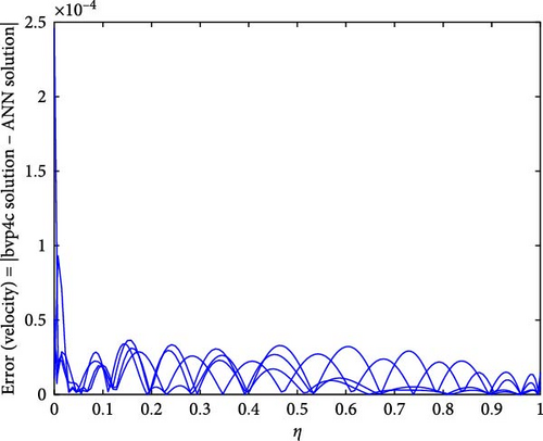
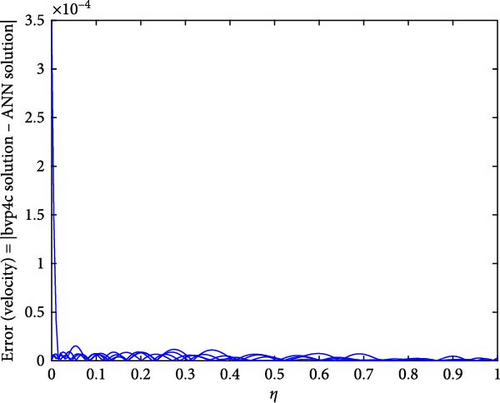
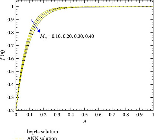
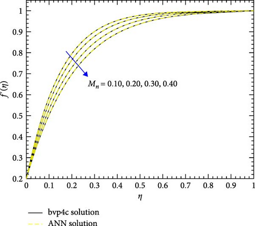
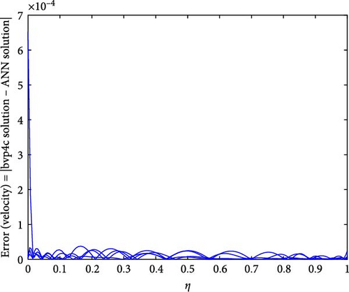
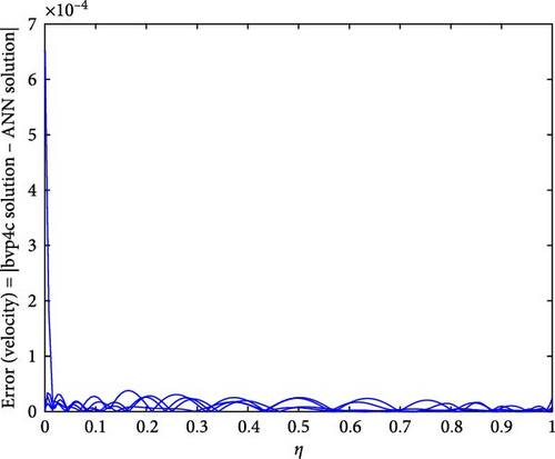
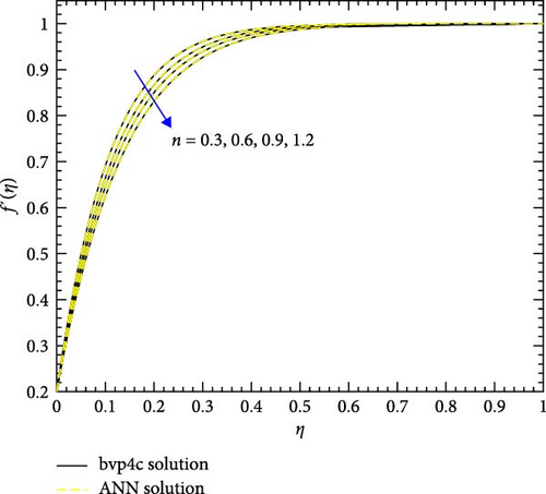
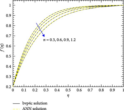
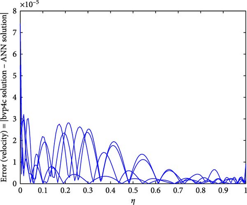
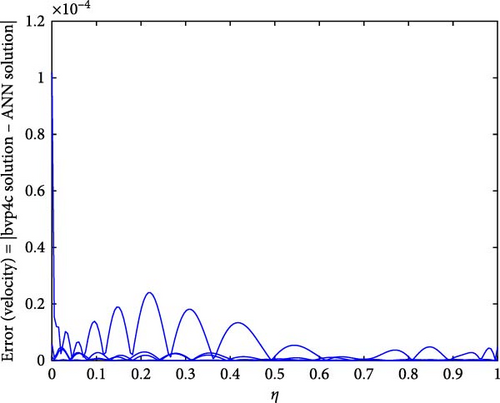
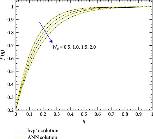
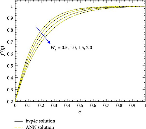
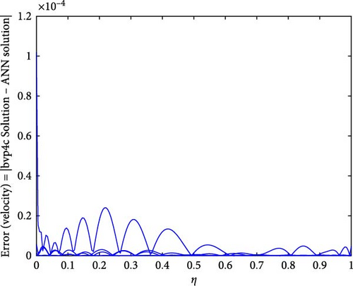

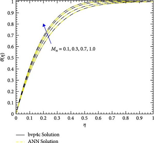
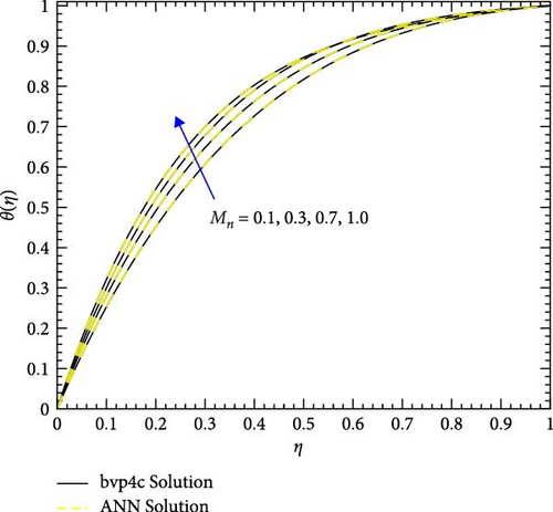
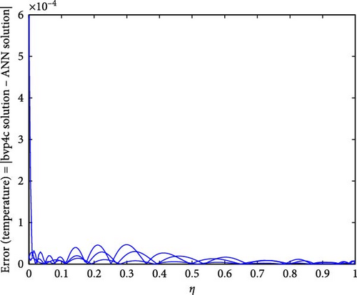
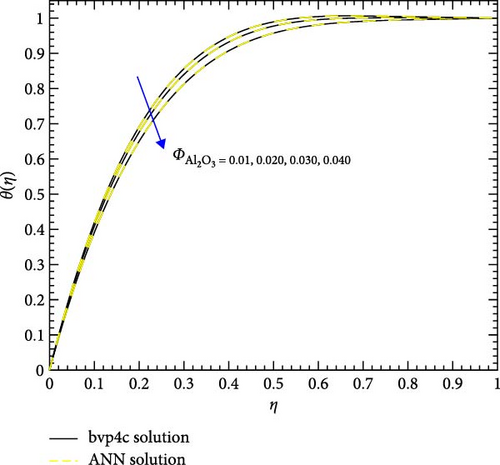
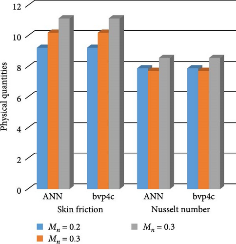
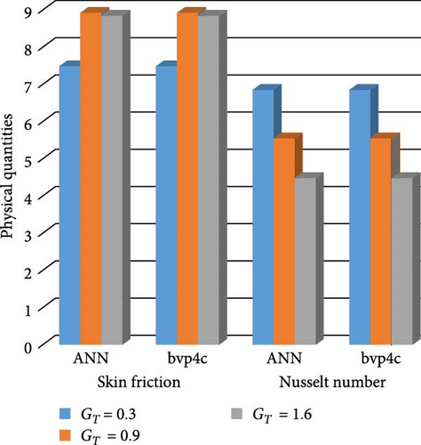
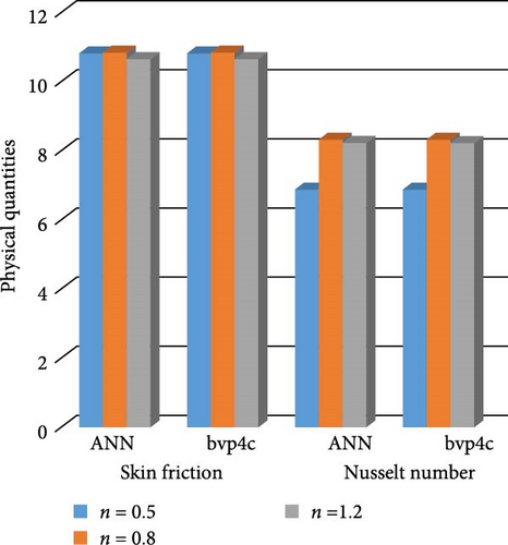
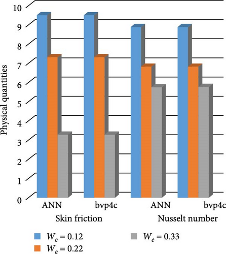
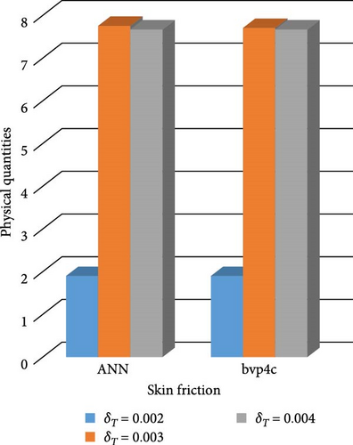
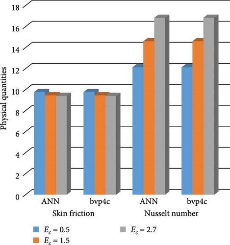
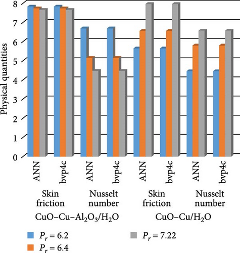
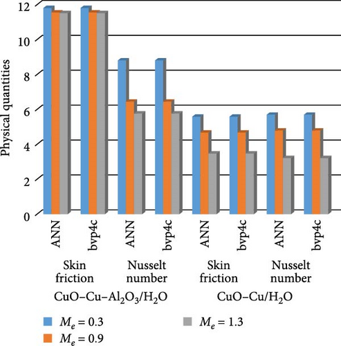
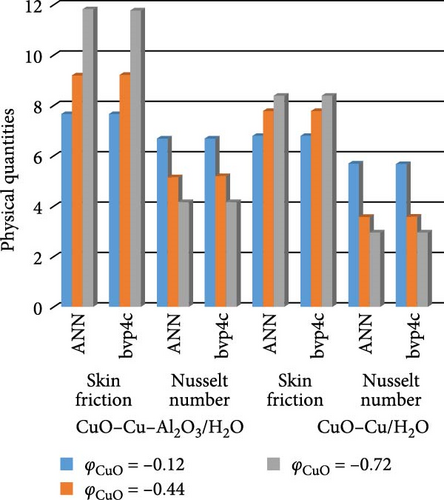
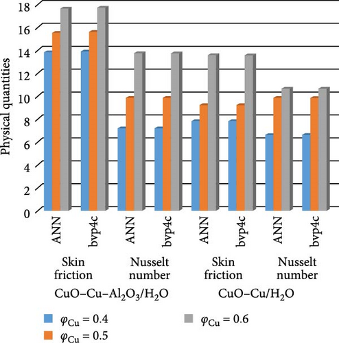
Figure 22a,b shows the impact of the thermal relaxation parameter on temperature of trihybrid and hybrid cross nanofluid flow, and Figure 23a,b shows error estimation between ANN and bvp4c. The temperature of a cross nanofluid increases with higher numerical values of the thermal relaxation parameter. In the presence of conductive nanoparticles, higher thermal relaxation parameter implies a slower adjustment of particle temperatures to variations in the local thermal environment. This delayed response leads to enhanced thermal resistance and a subsequent rise in the fluid temperature. The slower relaxation of particle temperatures hinders efficient heat dissipation, causing an accumulation of thermal energy within the fluid. Consequently, as the thermal relaxation parameter increases, so does the fluid temperature, making this parameter crucial in understanding and optimizing heat transfer processes in applications involving conductive nanoparticles, like in advanced thermal management systems or nanofluid-based heat exchangers. Figure 24a,b shows the impact of the Hartmann parameter on the temperature of trihybrid and hybrid cross nanofluid flow, and Figure 25a,b shows error estimation between ANN and bvp4c. The temperature profile of cross nanofluid increases with higher numerical values of Hartmann parameter due to the interaction between magnetic fields and electrically conductive particles. In the presence of CuO, Cu, and Al2O3 nanoparticles, these particles experience increased magnetic forces, velocity gets slower, and temperature gets high. Figure 26a,b shows the impact of volume fraction of Al2O3 on temperature of trihybrid and hybrid cross nanofluid flow, and Figure 27a,b shows error estimation between ANN and bvp4c. The temperature of a cross nanofluid becomes lower with an increasing numerical values of volume fraction of Al2O3 because this has a higher thermal conductivity as compared to the base fluid. This numerical increment in volume fraction of Al2O3 increases, the number of particles in the fluid also increases which leads to more efficient transfer of heat. Therefore, the temperature of the fluid decreases as the volume fraction of Al2O3 increases. Figure 28a,b shows the impact of volume fraction of CuO and Cu on temperature of trihybrid and hybrid cross nanofluid flow, and Figure 29a,b shows error estimation between ANN and bvp4c. The decrease in temperature of cross nanofluid is seen with increasing the numerical values of volume fraction of CuO and Cu. Due to the high thermal conductivity of CuO and Cu, the overall thermal conductivity of the fluid also rises and consequently fluid becomes more proficient at transferring heat away from the system and that leads to reduction in temperature. Table 7 explains the numerical outcome of skin friction and Nusselt Number estimation for CuO─Cu/H2O with variation of physical parameters with the help of both techniques ANN and bvp4c. Tables 8 and 9 presents skin friction and Nusselt number estimation for CuO─Cu─Al2O3/H2O and CuO─Cu─Al2O3/H2O and CuO─Cu/H2O. The statistical representation is shown in Figures 30a,b–35.


| Mn | GT | Ec | n | We | δT | Ec | CuO─Cu/H2O | |||
|---|---|---|---|---|---|---|---|---|---|---|
| Skin friction | Nusselt number | |||||||||
| ANN | bvp4c | ANN | bvp4c | |||||||
| 0.1 | — | — | — | — | — | — | 7.564567 | 7.567383 | 6.6433456 | 6.643731 |
| 0.2 | — | — | — | — | — | — | 8.937876 | 8.932354 | 6.6784365 | 6.678452 |
| 0.3 | — | — | — | — | — | — | 9.76666 | 9.768952 | 5.9036643 | 5.908754 |
| — | 0.3 | — | — | — | — | — | 2.781666 | 2.781542 | 5.8776655 | 5.879773 |
| — | 0.9 | — | — | — | — | — | 3.7894532 | 3.7849411 | 5.89123443 | 5.8597516 |
| — | 1.6 | — | — | — | — | — | 4.4564568 | 4.4564711 | 3.67433535 | 3.6715176 |
| — | — | π/6 | — | — | — | — | 5.9672652 | 5.9644789 | 6.85556446 | 6.8615412 |
| — | — | π/4 | — | — | — | — | 4.1907664 | 4.190t863 | 6.99867544 | 6.9730742 |
| — | — | π/3 | — | — | — | — | 3.8798665 | 3.8765541 | 6.76477646 | 6.7869051 |
| — | — | — | 0.3 | — | — | — | 6.9764787 | 6.9067651 | 7.76676473 | 7.7865189 |
| — | — | — | 0.6 | — | — | — | 5.6575782 | 5.6513902 | 7.5375755 | 7.5688489 |
| — | — | — | 0.9 | — | — | — | 3.8987863 | 3.8953461 | 7.6536368 | 7.6548741 |
| — | — | — | — | 0.12 | — | — | 6.1787576 | 6.1783542 | 5.3275145 | 5.3278891 |
| — | — | — | — | 0.22 | — | — | 4.1765764 | 4.1574853 | 4.5654172 | 4.5678109 |
| — | — | — | — | 0.33 | — | — | 3.8653543 | 3.8974644 | 3.8712456 | 3.8758461 |
| — | — | — | — | — | 0.0002 | — | 6.1764622 | 6.1984652 | — | — |
| — | — | — | — | — | 0.0003 | — | 6.1578665 | 6.1574652 | — | — |
| — | — | — | — | — | 0.0004 | — | 6.1467876 | 6.145678 | — | — |
| — | — | — | — | — | — | 0.5 | 5.787672 | 5.7684971 | 6.78943446 | 6.7898424 |
| — | — | — | — | — | — | 1.5 | 3.175646 | 3.1454643 | 8.45436243 | 8.4516082 |
| — | — | — | — | — | — | 2.7 | 2.787565 | 2.7845691 | 11.1423624 | 11.190854 |
- Abbreviations: ANN, artificial neural network; bvp4c, boundary value problem of a fourth-order; Cu, copper; CuO, copper oxide.
| Mn | GT | Ec | n | We | δT | Ec | CuO─Cu─Al2O3/H2O | |||
|---|---|---|---|---|---|---|---|---|---|---|
| Skin friction | Nusselt number | |||||||||
| ANN | bvp4c | ANN | bvp4c | |||||||
| 0.2 | — | — | — | — | — | — | 9.203455 | 9.2007242 | 7.853456464 | 7.85432671 |
| 0.3 | — | — | — | — | — | — | 10.184563 | 10.189381 | 7.715678953 | 7.71464561 |
| 0.3 | — | — | — | — | — | — | 11.135678 | 11.133245 | 8.545678544 | 8.54434914 |
| — | 0.3 | — | — | — | — | — | 7.4756754 | 7.4759708 | 6.85445677 | 6.85432915 |
| — | 0.9 | — | — | — | — | — | 8.91516544 | 8.91513444 | 5.548746532 | 5.544426735 |
| — | 1.6 | — | — | — | — | — | 8.8458765 | 8.84583421 | 4.483253462 | 4.483355564 |
| — | — | π/6 | — | — | — | — | 9.99755675 | 9.99754223 | 9.942354646 | 9.942606579 |
| — | — | π/4 | — | — | — | — | 9.47567823 | 9.47977421 | 9.832354657 | 9.832165534 |
| — | — | π/3 | — | — | — | — | 9.48245678 | 9.48297698 | 9.751567353 | 9.751655545 |
| — | — | — | 0.5 | — | — | — | 10.7956785 | 10.7978254 | 6.853235456 | 6.853256567 |
| — | — | — | 0.8 | — | — | — | 10.8456783 | 10.8436476 | 8.321234545 | 8.321378592 |
| — | — | — | −0.5 | — | — | — | 10.6345674 | 10.6547714 | 8.206q23454 | 8.206365545 |
| — | — | — | — | 0.12 | — | — | 9.47678961 | 9.47449472 | 8.852345454 | 8.853267532 |
| — | — | — | — | 0.22 | — | — | 7.30345678 | 7.30324469 | 6.812345656 | 6.819855578 |
| — | — | — | — | 0.33 | — | — | 3.2434567 | 3.2481435 | 5.733245654 | 5.749756554 |
| — | — | — | — | — | 0.0002 | — | 1.8989543 | 1.8914241 | — | — |
| — | — | — | — | — | 0.003 | — | 7.756786 | 7.7044546 | — | — |
| — | — | — | — | — | 0.004 | — | 7.6704325 | 7.6703565 | — | — |
| — | — | — | — | — | — | 0.5 | 9.7084543 | 9.70874871 | 12.10123452 | 12.10245689 |
| — | — | — | — | — | — | 1.5 | 9.4294565 | 9.42981654 | 14.5634564 | 14.56766564 |
| — | — | — | — | — | — | 2.7 | 9.3984321 | 9.39815642 | 16.7845676 | 16.78646565 |
- Abbreviations: Al2O3, aluminum oxide; ANN, artificial neural network; bvp4c, boundary value problem of a fourth-order; Cu, copper; CuO, copper oxide.
| Pr | Me | λ | φCuO | φCu | CuO─Cu─Al2O3/H2O | CuO─Cu/H2O | |||||||
|---|---|---|---|---|---|---|---|---|---|---|---|---|---|
| Skin friction | Nusselt number | Skin friction | Nusselt number | ||||||||||
| ANN | bvp4c | ANN | bvp4c | ANN | bvp4c | ANN | bvp4c | ||||||
| 6.2 | — | — | — | — | — | 7.8245433 | 7.8234032 | 6.672340 | 6.675432 | 5.63242 | 5.671198 | 4.442579 | 4.44453 |
| 6.4 | — | — | — | — | — | 7.7255332 | 7.7237648 | 5.123459 | 5.125478 | 6.54544 | 6.565163 | 5.786432 | 5.78454 |
| 7.22 | — | — | — | — | — | 7.6487576 | 7.6432901 | 4.462345 | 4.467913 | 7.95444 | 7.951671 | 6.561966 | 6.56453 |
| — | 0.3 | — | — | — | — | 11.787685 | 11.785671 | 8.786548 | 8.785331 | 5.56544 | 5.567802 | 5.678214 | 5.67854 |
| — | 0.9 | — | — | — | — | 11.548756 | 11.542885 | 6.445645 | 6.456713 | 4.67544 | 4.671541 | 4.781026 | 4.78154 |
| — | 1.3 | — | — | — | — | 11.487667 | 11.456795 | 5.753456 | 5.756818 | 3.46677 | 3.461373 | 3.205751 | 3.20443 |
| — | — | — | −0.12 | — | — | 7.6548756 | 7.6547891 | 6.673245 | 6.670052 | 6.76654 | 6.764024 | 5.675414 | 5.67543 |
| — | — | — | −0.44 | — | — | 9.1776423 | 9.1749085 | 5.132456 | 5.156781 | 7.76776 | 7.754635 | 3.567768 | 3.56434 |
| — | — | — | −0.72 | — | — | 11.797698 | 11.768901 | 4.142345 | 4.146371 | 8.37765 | 8.378936 | 2.943069 | 2.94334 |
| — | — | — | — | 0.4 | — | 13.809876 | 13.874332 | 7.163245 | 7.167358 | 7.81234 | 7.830285 | 6.617401 | 6.61344 |
| — | — | — | — | 0.5 | — | 15.534567 | 15.569321 | 9.823400 | 9.876501 | 9.17945 | 9.189228 | 9.854962 | 9.85346 |
| — | — | — | — | 0.6 | — | 17.609876 | 17.673071 | 13.73245 | 13.71563 | 13.5692 | 13.57571 | 10.65917 | 10.6578 |
| — | — | — | — | — | 0.3 | 11.687654 | 11.675432 | 4.872134 | 4.879041 | — | — | — | — |
| — | — | — | — | — | 0.5 | 13.909876 | 13.905431 | 5.023400 | 5.031784 | — | — | — | — |
| — | — | — | — | — | 0.6 | 16.519876 | 16.510784 | 8.467213 | 8.467381 | — | — | — | — |
- Abbreviations: Al2O3, aluminum oxide; ANN, artificial neural network; bvp4c, boundary value problem of a fourth-order; Cu, copper; CuO, copper oxide.
Figure 30a,b shows magnetic and local Grashof temperature number on physical quantities. Figure 31a,b shows the impact of cross-fluid index and Weissenberg number on physical quantities. Figure 32a,b interprets the impact of thermal relaxation and Ec on physical quantities. Figure 33a,b statistically interpret the impact of “Pr” and “We” on physical quantities. Figure 34a,b depicts the impact of volume friction of Cu and CuO on physical quantities. Finally, Figure 35 explores the impact of volume friction of Al2O3 on physical quantities.
9. Conclusions
- 1.
The best numerical value for performance is 3.0999e-09 at 357 epochs in the case of a cross-fluid index, 4.1816e-11 at 267 epochs for the Hartmann parameter, and 4.7122e-11 at 303 epochs for the thermal relaxation parameter.
- 2.
The numerical output values of gradient, mu, and validation checks estimation during ANN training for variation three physical parameters are (mu 1e-08, 1e-09, and 1e-09) and gradient are 9.96e-08, 9.9234e-08, 9.9326e-08, and (0, 0, 0) are the numerical values of validation checks.
- 3.
The velocity of a fluid is observed to decrease with an increase in the Weissenberg number due to enhanced viscoelastic properties in the presence of nanoparticles (Cu, CuO, and Al2O3).
- 4.
The Hartmann parameter tends to decrease the velocity of the fluid due to magnetic field strength is produced with higher Hartmann numbers and this magnetic field exerts a drag force on the conductive fluid containing the suspended nanoparticles.
- 5.
The velocity of fluid decreases with increasing values of the melting parameter in the presence of Cu, CuO, and Al2O3 nanoparticles. When melting parameter increases, the nanoparticles tend to exhibit higher melting points, leading to enhanced thermal stability and hence temperature decreases.
- 6.
The decrease in the velocity of fluid is found with increasing values of the local Grashof temperature number in the presence of Cu, CuO, and Al2O3 nanoparticles because this is related to buoyancy-induced flow within a fluid adjacent to a heated or cooled surface.
- 7.
The decrease in temperature of a fluid with increasing volume fraction of CuO and Cu because when the volume fraction of CuO and Cu increases, the overall thermal conductivity of the fluid also rises and cause in reduction of temperature.
- 8.
The temperature of a fluid tends to increase with increasing values of the Hartmann parameter in the presence of CuO, Cu, and Al2O3 due to the interaction between magnetic fields and electrically conductive particles.
- 9.
The temperature of a fluid tends to increase with increasing values of the thermal relaxation parameter in the presence of CuO, Cu, and Al2O3 due to the impact of thermal relaxation processes on heat transfer.
9.1. Future Work Direction
- 1.
Fluid can be considered on a paraboloid surface with some distinct types of nanoparticles.
- 2.
The impact of the heat source/sink, two-phase model along with Joule heating is also considered in the extension of this work.
- 3.
A combination of ANN and finite difference methods can be applied to this model.
Nomenclature
-
- T0:
-
- Solid surface temperature
-
- T∞:
-
- Free stream temperature
-
- T:
-
- Fluid temperature
-
- β0:
-
- Magnetic field strength
-
- Cs:
-
- Solid surface-specific heat
-
- ω:
-
- Acute angle
-
- Tri − nf:
-
- Trihybrid nanofluid
-
- Base − f:
-
- Base fluid
-
- ΦCu:
-
- Volume friction of copper
-
- αT:
-
- Thermal diffusivity
-
- Cp:
-
- Specific heat at constant pressure
-
- βT:
-
- Thermal expansion coefficient
-
- ρ:
-
- Density
-
- n:
-
- Flow index or cross model index
-
- f:
-
- Nondimensional profile of velocity
-
- Mn:
-
- Hartmann parameter
-
- Pr:
-
- Prandtl number
-
- Ec:
-
- Eckert number
-
- Me:
-
- Melting parameter
-
- Nux:
-
- Nusselt number
-
- qw:
-
- Heat transfer rate
-
- Tm:
-
- Melting point temperature
-
- u, v:
-
- Velocity components
-
- Γ:
-
- Time relaxation constant
-
- g:
-
- Gravitational acceleration
-
- L:
-
- Latent heat
-
- λT:
-
- Thermal relaxation constant
-
- Hy − nf:
-
- Hybrid nanofluid
-
- ΦCuO:
-
- Volume friction of copper oxide
-
- :
-
- Volume friction of aluminum oxide
-
- ρCp:
-
- Heat capacity
-
- σ:
-
- Fluid electrical conductivity
-
- k:
-
- Fluid thermal conductivity
-
- μ:
-
- Dynamic viscosity of fluid
-
- η:
-
- Similarity variable
-
- θ:
-
- Nondimensional profile of temperature
-
- GT:
-
- Local Grashof parameter
-
- δT:
-
- Thermal relaxation parameter
-
- λ:
-
- Shrinking parameter
-
- Cf:
-
- Skin friction
-
- τ:
-
- Shear stress
-
- Rex:
-
- Reynolds numbers
-
- We:
-
- Weissenberg number.
Conflicts of Interest
The authors declare no conflicts of interest.
Author Contributions
Syed Zahir Hussain Shah and Hafiz Abdul Wahab: conceptualization. El-Sayed M. Sherif, Syed Zahir Hussain Shah, Anuar Ishak, and Umair Khan: methodology. Shabbir Ahmad, Anuar Ishak, Hafiz Abdul Wahab, Syed Zahir Hussain Shah, and Umair Khan: software. Syed Zahir Hussain Shah, Shabbir Ahmad, Muhammad Sajjad, Umair Khan, Hafiz Abdul Wahab, and Anuar Ishak: validation. El-Sayed M. Sherif, Syed Zahir Hussain Shah, Anuar Ishak, Muhammad Sajjad, Shabbir Ahmad, and Hafiz Abdul Wahab: formal analysis. Anuar Ishak and Hafiz Abdul Wahab: investigation. Anuar Ishak: resources. Anuar Ishak, Hafiz Abdul Wahab, Umair Khan, and Muhammad Sajjad: data curation. El-Sayed M. Sherif, Shabbir Ahmad, Umair Khan, and Muhammad Sajjad: writing–original draft preparation. El-Sayed M. Sherif, Shabbir Ahmad, and Muhammad Sajjad: writing–review and editing. Hafiz Abdul Wahab: visualization. Anuar Ishak: supervision. El-Sayed M. Sherif: project administration, funding acquisition. All authors have read and agreed to the published version of the manuscript.
Funding
This research has been supported by the Universiti Kebangsaan Malaysia Project Number “DIP-2023-005.” Also, the authors extend their appreciation to the Researchers Supporting Project Number (RSP2024R33), King Saud University, Riyadh, Saudi Arabia.
Acknowledgments
This research has been funded by the Universiti Kebangsaan Malaysia Project Number “DIP-2023-005”. Also, the authors extend their appreciation to the Researchers Supporting Project Number (RSP2024R33), King Saud University, Riyadh, Saudi Arabia.
Open Research
Data Availability Statement
The datasets used and/or analyzed during the current study are available from the corresponding author upon reasonable request.


