1. Introduction

Submarine-launched projectile refers to a projectile launched by a submarine as a launching platform. Compared with fixed or mobile launching platforms on land, submarines have stronger maneuverability, larger combat killing radius, higher survivability, and better concealment. Submarine-launched projectiles have the characteristics of wide range coverage, accurate strike on targets, and strong deterrence and destruction. On this basis, submarine-launched projectile combines the advantages of submarine and projectile, making it an important weapon in modern warfare [1]. Compared to fixed or mobile launch platforms on land, submarines are more mobile, have a larger operational kill radius, are more survivable, and are more concealable. Submarine-launched projectiles have a wide range, can strike targets with precision, and are extremely deterrent and destructive. It is on this basis that submarine-launched projectiles combine the advantages of both submarines and projectiles, making them an important weapon in modern warfare. Submarine-launched projectiles operate across two different media, water and air, and the dynamics of underwater launch differ significantly from those of air launch, with the differences in launch environment presenting many mechanical, structural, and control challenges [2].

Submarines can launch projectiles both on the surface and underwater [3]. Because submarine-launched projectiles operate in a much different environment to land- and air-launched projectiles, with underwater out-of-barrel and out-of-water processes, it is vital to be able to accurately predict the launch motion patterns of submarine-launched projectiles in different environments. There are currently experimental studies, theoretical studies, and numerical simulations to study the motion of submarine-launched projectile launches. Experimental and theoretical studies are limited by model size, funding, and measurement accuracy and are gradually being replaced by numerical simulation methods.

Numerical simulations of the underwater launch process of submarine-launched projectiles have been carried out by many scholars. Ge et al. [4], Li et al. [5], Liu and Ma [6], and Song [7] used MATLAB as the basic tool to simulate different underwater navigational bodies to study the motion patterns of different types of bodies, respectively. Cheng and Liu [8], Kunz et al. [9], and others applied multiphase CFD with implicit, preconditioning algorithms and dynamic mesh techniques to study the launching process of navigable bodies with different velocities. Lan et al. [10], Li [11], and Lu [12] used the commercial CFD software Fluent to numerically simulate the motion process of the vertical launch of the underwater navigable body, including the two phases of exit from the tube and exit from the water, respectively, and relevant experiments were also conducted to verify the accuracy of the simulation results.

As computational fluid dynamic technology continues to mature and develops, numerical simulation has become an important tool for studying many complex problems, but depending on the performance of the computer and the number of meshes and CPU core time, high-precision numerical simulation of the motion patterns of underwater navigable bodies is still very costly, so motion prediction based on reduced order method (ROM) has become an important research direction.

The commonly used methods for reduced order modelling include proper orthogonal decomposition (POD) and dynamic mode decomposition (DMD). The basic idea of such methods is decomposing the complex physics into the summation of different orders of modes, and each mode is composed of the space-dependent part (normally called mode functions) and their corresponding time coefficients. These techniques have been used for many problems such as the flow field and pressure field around stationary or oscillating cylinder [13]. It has also been applied for the problems with deformed or moving domain, in which the nonphysical quantities such as volume of fraction [14] or ALE mesh field [15] are decomposed by such reduced order models to deal with the problems of moving fluid and structure surface.

The important features of such decompositions are that the space-dependent part would normally be the same for scenarios under a large span of parameters. Therefore, once these space-dependent parts are extracted based on the data from scenarios under typical but limited number of parameters, the complex physics under the whole range of parameter space can be reconstructed based on these known space-dependent parts. For the cases that correspond to system parameters that are not in the database, the modal coefficients are obtained by machine learning or simple interpolating among the time coefficients from the known cases [14, 16], and these “unsimulated” cases can be recovered based on the known space-dependent parts and these predicted time coefficients. This means the direct simulation for all the potential parameter is not necessary, which can save significant amount of time.

In this paper, the abovementioned idea is applied to the forecasting of projectile velocity during the initial phase of launching (which is the most dynamic and important part of the whole launching process). The paper is organized as follows: Section 2 briefly introduces POD method and the principles of machine learning. Section 3 verifies the accuracy of the direct CFD numerical simulation model. Section 4 compares the results of the motion prediction with the CFD calculations to verify the accuracy of the motion prediction based on the reduced order model. The conclusion is drawn in Section 5.

2. ROM Model—POD and Machine Learning

2.2. Machine Learning

Machine learning is a general term for a class of algorithms. These algorithms attempt to mine hidden rules from a large amount of historical data and use them for prediction or classification. More specifically, machine learning can be seen as finding a function, where the input is sample data and the output is the desired result, but this function is too complicated to be formally expressed. It should be noted that the goal of machine learning is to make the learned functions well applicable to “new samples,” rather than just performing well on the training samples.

Machine learning is mainly divided into supervised learning, semisupervised learning, unsupervised learning, and reinforcement learning. Commonly used supervised learning algorithms include K-nearest neighbor algorithm, linear regression, logistic regression, support vector machine, decision tree, random forest, and neural network. The machine learning used in this paper is neural net fitting neural network that comes with MATLAB toolbox.

As shown in Figure 1, the neural network fitting is a feedforward neural network, which basically consists of an input layer, multiple hidden layers, and an output layer. It can fit multidimensional mapping problems arbitrarily, as long as there are consistent data and enough neurons in its hidden layers. There is no cycle in its operation, and information can only flow forward.

The abovementioned machine learning tool is used for the prediction of time coefficient under “unsimulated” cases. Then, the concerned value (i.e., the motion time history of the projectile in this work) can be reconstructed based on the “known” POD mode functions and “predicted” time coefficients. The neural net fitting tool in MATLAB toolbox is adopted for the implementation of the abovementioned neural network model.

3. The Simulation Method—CFD

The input data for the POD analysis and time coefficient prediction of the abovementioned ROM model is from CFD simulation, and the model settings are illustrated and validated in this section.

3.1. Geometric Model

As shown in Figure 2, the whole computational domain is under water (the top of the domain is at the depth of 15 m under water), and the projectile is initially placed in the center of the launcher, with the bottom of the projectile 100 mm away from the bottom of the launcher. The depth of the launcher is 30 m, and the initial position of the bottom of the piston is 3.5 m away from the launcher. The projectile is pushed upwards under the influence of the downward movement of the piston. The piston chamber and projectile launching chamber are connected through the connection valve.

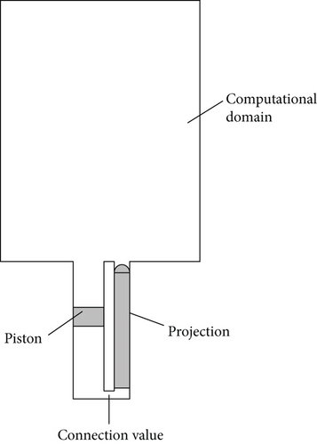
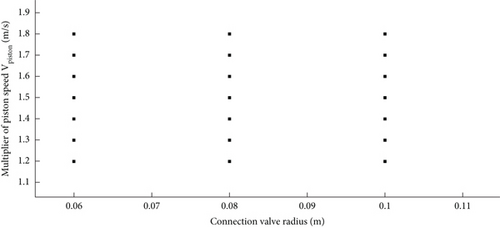
This launching process with different pipeline cross-sections and different piston velocity curves is simulated by two-dimensional CFD. The varying parameters are chosen to be velocity of the piston and the radius of the connection valve. The specific computational parameter matrix is shown in Figure 3. All these cases will be divided as two groups (i.e., training and forecasted groups, respectively). The data from training group is used for the ROM analysis as mentioned in Section 2. The resultant ROM model is then used to predict the results for forecasted group scenarios and cross-validate with the results by direct CFD simulation.

It has to be noted that the piston speed V_piston is the results of Equation (5) times the multiplier in Figure 3 for each particular case.

$$ ()

Other necessary geometrical parameters for computation are listed in Table 1.

Table 1. Geometrical parameters for launching computation.

Parameters	Value
Piston radius	794 mm
Piston barrel gap	3 mm
Projectile radius	300 mm
Projectile height	7000 mm
Projectile quality	1500 kg
Projectile tube gap	8 mm

3.3. Boundary Conditions and Other Settings

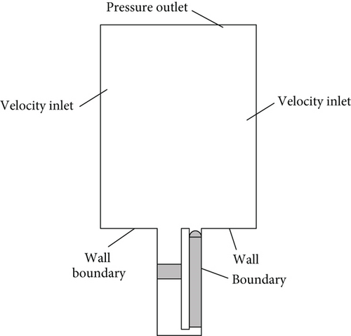
As shown in Figure 4(a), the boundary conditions are as follows: the left and right sides of the calculation domain are set as velocity inlets, the top is set as pressure outlets, the pressure at the pressure outlets is the pressure at the water depth of 15 m, and the rest are set as wall surfaces. The implicit time advancing method is used, and the time step is chosen to be 0.001 s. The pressure and velocity is coupled by SIMPLE method.

3.4. Grid Independence Verification

Grid division (see Figure 4) follows the following principles [2]:

• 1.

  The integral grid is dense enough, and there is no grid dependence in the solution.

• 2.

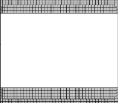
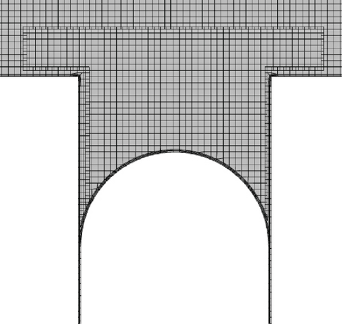
  Overlapping grid technology (overlapping grid is also called “nested” grid) is applied to discrete computing domains with multiple different grids overlapping each other in any way. These grids are the most useful when dealing with problems involving multiple bodies or moving bodies and in optimization research, and mesh encryption is carried out at piston, channel, and projectile, respectively.

• 3.

  The prismatic layer of the projectile coincides with the cylinder prismatic layer, the piston coincides with the piston cylinder prismatic layer, and the overlapping prism layers are three.

As the results of numerical simulation are directly related to grid division, in order to verify the accuracy of CFD numerical simulation, this part uses multiple sets of grids to verify the grid convergence for the standard conditions of the launch process (i.e., the diameter of the connection valve is 160 mm). The specific parameters of the grid are shown in Table 2.

Table 2. Grid parameter.

Grid type	Base size (m)	Number (million)	Time (min)
Rough	0.10	33	80
Suitable	0.08	51	300
Precision	0.04	203	490

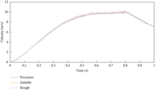
The calculation results of the three grids are similar. Considering the number of grids and the cost of calculation time, the other numerical simulation conditions in this paper all adopt moderate grids; that is, the basic size of grids is 0.08 m. Figure 5 shows the time-history curves of projectile velocity of three grids. As shown in the figure, the trend of the time-history curves of projectile velocity calculated by three grids is consistent, and the numerical fluctuation is small, which shows the accuracy of the numerical simulation in this paper, and the calculation results can be used for subsequent research.

4. Results and Discussions

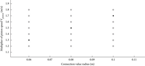
All the computations in Figures 3 and 6 are conducted by using the moderate grid in Table 2, among which 18 working conditions are selected for data training, and the other three working conditions are used to verify the accuracy of the machine learning model.

The POD analysis is applied for the data from the 18 training cases (Figure 6), and then, the resultant mode function Φ and their corresponding time coefficients a are obtained. Next, by using the conditions of these cases (i.e., the speed and radius values of these cases) as input and the time coefficients a as output data, the hidden relations between input and output data can be established by the neural network model mentioned in Section 2.2. More specifically, the number of hidden neurons network is chosen as the default value (i.e., 10). The algorithm used in training is Bayesian regularization. More specifically, 90% of the training data is selected for model training (i.e., 16 cases), 5% data for verification (i.e., one case), and 5% data for testing (i.e., one case). The MSE of the trained model is about 6e − 3.

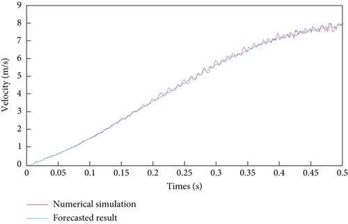
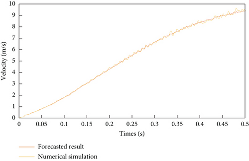
Based on the established prediction model, the time coefficients for the cases in the forecasted group can be obtained. The projectile velocity time history can then be recovered by combining the known POD mode functions and the predicted time coefficients as in Equations (2) and (3). Figure 7 shows the comparison data between machine learning forecast and direct CFD numerical simulation results under three working conditions. In terms of accuracy, it can be seen that the prediction results are very close to those from direct CFD simulation, which proves the reliability of the proposed method. For computational time, the direct CFD simulation for each case will take about 12 CPU hours, whereas the ROM model only takes negligible computational time. This means if the physics under a large range of parameters is of concerned, the cost of using ROM model is only a limited number of direct simulations with typical parameters instead of the direct simulation for the whole parameter range.

5. Conclusions

In order to accurately and quickly forecast the projectile launch velocity in the initial stage under different conditions, a ROM model that combines POD modal decomposition and neural network fitting is developed. The prediction results are compared with the results of direct CFD simulations, and it agrees well with each other, thus demonstrating the reliability and feasibility of the ROM, which also reduces significant amount of simulation time.

Conflicts of Interest

The authors declare no conflicts of interest.

Author Contributions

Conceptualization, methodology, validation, investigation: D.K., J.Y., and L.H.X. Resources: J.Y. Writing—original draft preparation: D.K. and L.H.X. Writing—review and editing: J.Y. All authors have read and agreed to the published version of the manuscript.

Funding

The authors received no specific funding for this work.