1. Introduction

Dengue fever is a virus-induced illness spread by mosquitoes rapidly in the tropical and subtropical regions throughout the globe in recent years. Female mosquitoes, mostly Aedes aegypti and, to a lesser degree, Aedes albopictus, transmit the dengue virus [1]. The risk levels of dengue fluctuate depending on rainfall, temperature, relative humidity, and unplanned rapid urbanization throughout the tropics [2]. Dengue fever is triggered by a virus belonging to the family Flaviviridae. The four distinct virus serotypes of dengue are DENV-1, DENV-2, DENV-3, and DENV-4 [1]. After recovering from an infection, it is believed that one will be impervious to that serotype for the remainder of their life. Cross-immunity to varying serotypes is insignificant [3]. Subsequent infections (secondary infections) with various serotypes increase the likelihood of severe dengue [4].

During the early outbreaks between 2000 and 2002, DENV-3 was identified as the predominant serotype although all four dengue serotypes were present [5]. Subsequently, there was a lack of data on serotype circulation until 2012. Reference [6] later demonstrated that DENV-1 and DENV-2 were the dominant serotypes circulating from 2013 to 2016. In 2017, DENV-3 reemerged after a period of dormancy, with DENV-2 remaining the most prevalent serotype. Since the major outbreak in 2019, DENV-3 has been the most frequently detected serotype. There is limited information on the genotypic diversity of dengue viruses, but three genotypes (I, II, and III) of DENV-3 and the cosmopolitan genotype of DENV-2 are currently found in Bangladesh [5]. The potential reemergence of the DENV-4 serotype, which has not been reported for over 2 decades, could present a significant public health risk in Bangladesh due to the possibility of secondary infections [5].

DENV-positive individuals are capable of infecting mosquitoes. This can include individuals with asymptomatic dengue infection, those who have not yet developed a symptomatic infection (presymptomatic), and healthy individuals (asymptomatic) [1]. Human-to-mosquito transmission can occur up to 2 days before the onset of symptoms [1, 7–11] and up to 2 days after the fever has gone away [12]. High viremia and fever in the patient are linked to a higher chance of mosquito infection; on the other hand, increased DENV antibodies are linked to lower chances of infection [12]. The majority of patients are viremic for 4–5 days although viremia can persist up to 12 days [13]. Mosquito vectors are the major route of transmission of DENV between people. There is evidence, however, that maternal transmission during pregnancy is possible. The vertical transmission of the disease despite its low risk is correlated with the timing of dengue infection during pregnancy. An infected mother [14–18] may give birth to a premature baby or an underweight baby or may have fetal distress [19].

One of the prime objectives of epidemic modeling is to devise ways to eliminate the disease. A fundamental principle of epidemiological modeling is that most models exhibit the threshold behavior of Ross, Kermack, and McKendrick, which asserts that a specific set of parameters dictates if an illness can infect and survive [20]. For this threshold, Diekmann in 1990 provided a fundamental biological concept that is still commonly used today [21]. The estimated number of secondary cases that a typical sick person will cause throughout a pathogen’s whole duration of infectiousness in a population that is susceptible was characterized as the pathogen’s basic reproductive number (BRN), which is commonly denoted by R₀ [21, 22]. It is advantageous to have an equation for R₀ since the BRN can provide information regarding epidemic outbreaks. This enables one to see how an individual model parameter can affect R₀ and what modifications one would need to make to stop an epidemic. R₀ offers additional information in addition to explaining this threshold behavior. The BRN can be utilized to figure out the volume of the susceptible population that has to be vaccinated in order to avoid an outbreak. In basic modeling techniques, for example, the illness can be eradicated by vaccinating 1 − 1/R₀ of the population [20, 23]. This provides public health authorities with a helpful tool for determining annual vaccination production for diseases such as influenza. A standard R₀ conclusion for vector-borne diseases is that the vector population must be divided by $$ to eradicate the disease [24]. $$, where $$ is the mean age of infection and $$ is the mean life expectancy for models with exponential age distribution [25]. As a result, R₀ may be utilized for more than simply determining the duration of an outbreak; it can also assist health professionals in relating crucial epidemiological quantities.

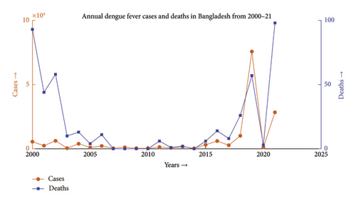
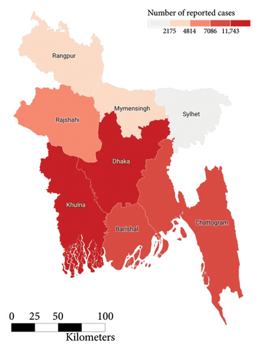
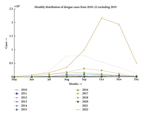
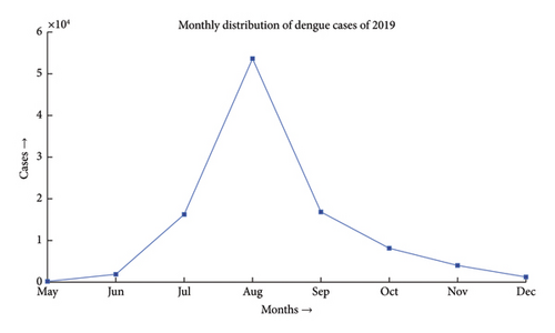
Dengue fever incidence varies with season, with the timing and size of seasonal peaks varying from year to year. These variations are driven by climate change and the associated variation in mosquito populations, as well as interannual fluctuation in DENV activity. Aedes aegypti and Aedes albopictus lay their eggs in containers that are filled with premonsoon rain in May, which causes an increase in the mosquito population. After the rainy season ends in September, mosquito numbers progressively decline. During the monsoon, the mean monthly temperature is almost always in a range that is conducive to mosquito growth and DENV transmission. National surveillance data typically show a rise in the incidence beginning in June and peaking in August, followed by a steady decrease, as depicted in Figures 1 and 2 [26]. The dengue scenario for the year 2022 is presented in Figure 3.

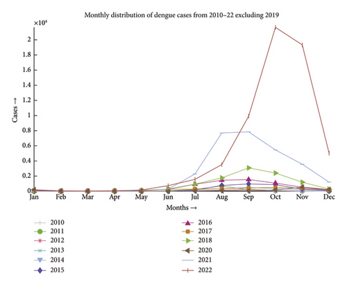
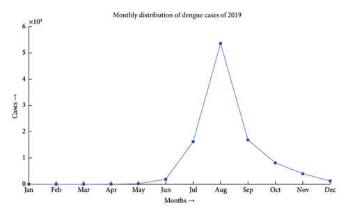
A close-up view of Figures 1 and 2 is included in Appendix A as Figures A1 and A2.

To simplify the model, some models with seasonal illnesses will only include one season at a time, essentially eliminating the seasonality element [27]. As seasonality plays a crucial role in the population dynamics of the disease, it must be accounted for in a model for a better study of the case. The incorporation of the seasonality can be accomplished in several ways. Forced oscillators are used in several modeling techniques to depict a wide variety of dynamics [27]. Making the transmission parameter periodic in time is the easiest approach to examining seasonality in models [28–30]. Other characteristics, such as birth or death rates for animals with mating seasons, can likewise be made periodic. This is not to suggest that seasonal forcing is suitable in every situation; in fact, applying this can render a model more complex and hard [27].

This paper aims to model the dengue scenario in Bangladesh using a nonautonomous, periodic, SIS vector–host model. To analyze the R₀ of this nonautonomous model, we propose some improvements over the existing linear operator method. We conduct a sensitivity analysis of the parameters considered for the models to determine the most prominent parameters to control disease dynamics for times to come.

2. Materials and Methods

2.1. Study Area

Bangladesh, situated near the mouth of the Bay of Bengal (Figure 4), encompasses a significant portion of the Bengal Delta, which has been shaped by the sediment deposition from the Ganges–Brahmaputra–Meghna (GBM) river system [32]. The GBM rivers carry the largest sediment load globally, primarily sourced from the Himalayan and Indo-Burman mountains [33], and they contribute to the fourth-highest volume of water discharge to the ocean [34]. The geographical coordinates of Bangladesh range from 20^°34^′N to 26^°38^′N and 88^°01^′E to 92^°41^′E [35].

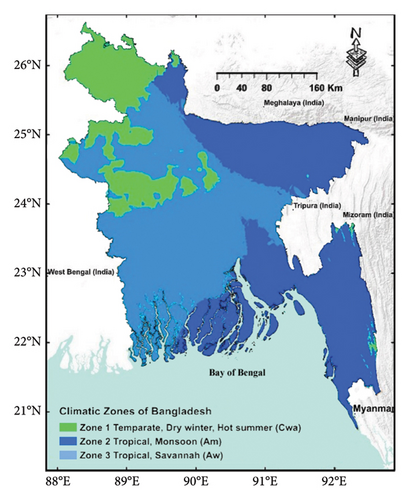
Bangladesh, located along the Tropic of Cancer, experiences a humid tropical/subtropical climate characterized by moderately warm temperatures, high humidity, and significant seasonal variations in rainfall patterns [36]. According to the Köppen–Geiger climate classification [31], the country encompasses three climate zones: temperate with a dry winter and hot summer (Cwa; Zone 1; Figure 4), tropical monsoon (Am; Zone 2), and tropical savannah (Aw; Zone 3). Annual rainfall averages 2300 mm, ranging from 1500 mm in the west to over 4000 mm in the northeast [37]. The mean temperature varies from 18°C to 22°C in winter and 23°C to 30°C in summer. Climate models predict a temperature increase of 2.4°C and a 9.7% increase in rainfall in Bangladesh by the end of the 21st century [38].

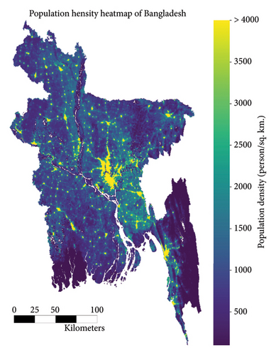
The population of Bangladesh as of 2022 is 171,186,372 [39]. A high-resolution demographic density map of the country is presented in Figure 5. The figure clearly exhibits the highest population density around the country’s capital city, Dhaka (the yellow-lit part in the middle of the country), followed by the port city of the country, Chattorgram (the yellow-lit part at the southeastern end of the country), and finally clusters around the different cities of the country. The population density slowly diminishes as we move away from the cities of the country. Dengue is a disease that often thrives in densely populated urban and tropical settings. Such has also been seen in the case of the heat map of the number of reported cases of dengue in 2022, as exhibited in Figure 3. Each of the polygons in the heat map represents each division (first of order of administrative level in the country) of Bangladesh. The heat map also shows that the intensity of DENV is higher in densely populated, highly urbanized regions in comparison to its sparsely populated, suburban counterparts.

Dengue has been a problem for Bangladesh since the beginning of this century, as illustrated in Figure 6. The problem was much more in control till the first decade. Due to higher technological advancements, rapid urbanization and industrialization, filling up of water bodies, and most importantly climate change, the problem has begun to move out of hand and the country has seen the horrid face of the problem in 2019 where the number of reported cases has gone over 50,000, which has been the maximum in the last 2 decades. The problem shows an upward trend, and the incident of 2019 may only be a glimpse of the problem this disease can pose in the upcoming decade.

2.3. Formulation of the Vector–Host Model

We wanted to exhibit the proposed linear operator model; hence, we have chosen a basic model to simulate the outcomes of the model as increased complexity in the model architecture can correlate with the increased symbolic computational complexity of the linear operator method.

Mathematical models are generally formulated based on some assumptions. The model considered here is a variation of the Ross 1911 second malaria model. The assumptions to formulate the model are as follows:

• 1.

  Two heterogeneous classes of the population are considered in the model. One is of the vector, and the other is of the host. Each of the classes is partitioned into two subclasses: susceptible and infected.

• 2.

  A susceptible host can only be infected by the infected vector and vice versa.

• 3.

  Total host population (N_h) and total vector population (N_v) are considered constant.

• 4.

  The vector and host population is nonimmune to the disease.

The following system of nonlinear, nonautonomous differential equations may be used to characterize the dynamics of this infectious disease in both host and vector populations:

$$ ()

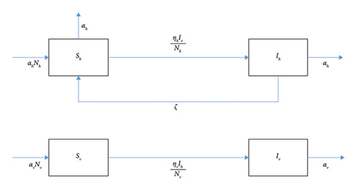
Here, prime ′ denotes the derivative with respect to the temporal variable, t. The parameter’s definition and values are discussed in Table 1. The flowchart of Model (1) is displayed in Figure 7.

Table 1. Parameter values are estimated from the mentioned data source.

Parameters	Definition	Values	Reference
ah	Off-season infection rate (host)	1.01396	Estimated
bh	Peak season infection rate (host)	9.05282	Estimated
av	Off-season infection rate (vector)	0.7875	Estimated
bv	Peak season infection rate (vector)	2.3625	Estimated
ζ	Recovery rate of host	[0, 1]	Estimated
τ	Length of peak season	5	[26]
ω	Length of each season	12	[26]
αh	Gross birth rate/per capita mortality rate (host)	[0, 0.0083]	[41]
αv	Gross birth rate/per capita mortality rate (vector)	[0, 2.459]	[42]
p	Vector-to-host ratio	[0, 0.0055]	[42]

• These are used to generate figures of the simulations.

Equation (1) has a feasibility region of $$ (the positive orthant of $$), and the system is well-posed. In order to normalize System (1), consider the following transformation: s_h = S_h/N_h, s_v = S_v/N_v, i_h = I_h/N_h, i_v = I_v/N_v, and p = N_v/N_h. Misusing the notations, S_h, S_v, I_h, and I_v we are left with

$$ ()

Here,

• •

  ζ denotes the recovery rate of the infected host.

• •

  α_h and α_v denote the birth rate or per capita natural mortality rate for the host and vector, respectively,

  $$ ()

•  

  denotes the rate at which susceptible hosts are infected by the vector.

  $$ ()
  denotes the rate at which susceptible vectors are infected by the host.

Clearly from the above definition we can say that both η_h(t) and η_v(t) are the square wave function of periodicity ω, where τ is the length of each season.

3. Numerical Simulation and Results

This evidently satisfies Assumption 6.

This evidently satisfies Assumption 7.

3.2. Parameter Estimation

In order to simulate the dengue scenario in Bangladesh using the model proposed in equation (2), we need to determine the values of the model parameter as per the scenario at hand. Values of τ, ω, α_h, α_v, and p are readily adopted from the prevalent literature. To estimate the values of the remaining parameters, we used the least square method whose methodological description can be found in Ref. [56]. The empirical number of reported cases on a month m, denoted as $$, and the number of incidences predicted by the model on month m, denoted as $$, are compared using the scaling parameter α introduced by Ref. [57]. The sum of squares error is then calculated as follows:

$$ ()

The parameter space is uniformly sampled utilizing the Latin hypercube sampling method [58] to produce parameter combinations. The detailed descriptions of the parameters and the corresponding Latin hypercube sampling ranges are presented in Table 1. Subsequently, we computed the sum of squares score using (25) for each parameter set over a simulation run. Following this, we employed the MATLAB GlobalSearch algorithm to identify the optimal parameter combinations by focusing on the parameter sets that yielded the minimum sum of squares values. To tackle the stochastic nature of this approach, the 30 best-performing parameter sets generated from the Latin hypercube sampling were used as the initial points for the MATLAB GlobalSearch algorithm. We repeat the entire procedure twice, once for the off-season and once for the peak season to estimate the relevant parameters. According to the parameter values mentioned in Table 1, we execute the aforesaid algorithm, which gives us the following graph.

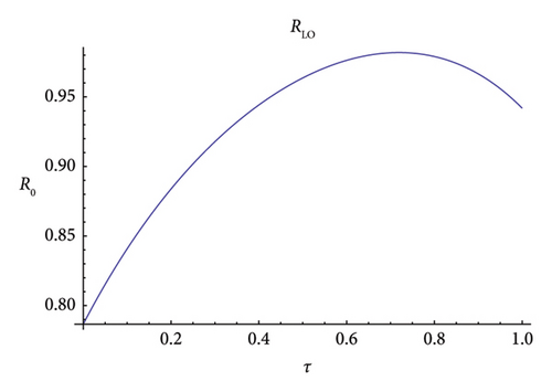
Figure 8 depicts the variation of R₀ with the variation of the length of the peak season, τ, using the linear operator method. It is evident that, for the variation of τ, R₀ is always below 1 but shows a peak in the interval of 7–9 months, and after 9 months, it shows a gradual decline. The graph is in agreement with the results of Refs. [27, 52] improving over the algorithm provided in it.

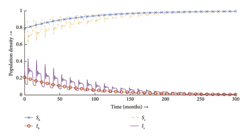
Now we plug in the value of parameters in the normalized system (2), which verifies the fact that DFE is stable and the infection dies out eventually (see Figure 9).

In nonautonomous cases like this, the classical time-average method has been seen to overplay or underplay the disease transmission risk [50] for the method relies on replacing periodic parameters, which in terms is not necessarily the original model. Contrary to the time-average method, it can be readily verified from Theorems C.1 and C.2 that the linear operator method by construction relies on the original model and hence provides the most accurate estimation of the disease transmission risk. Although the linear operator method in cases provides a very accurate depiction of R₀ in comparison to the time-average method, it is often more troublesome to be executed but can be executed in much more complicated cases compared to the time-average method [27, 52].

3.3. Sensitivity Analysis

Sensitivity analysis shows the influence of model parameters that have the greatest impact on the model’s dynamics. Using such analysis, epidemiologists can anticipate the critical parameters that play a critical role in disease-spreading dynamics.To determine the sensitivity of each parameter, we compute the partial rank correlation coefficient (PRCC) of each of the parameters with the data generated in the case of each compartments. The result is presented in Figure 10. The output will be considered statistically significant if the p value is less than 5%.

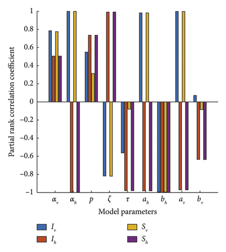
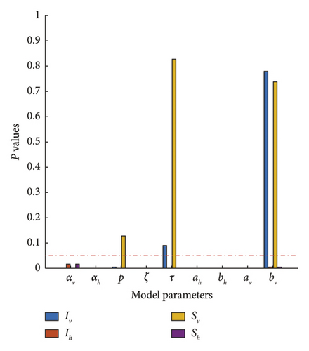
From Figure 10, we can deduce that the most impactful parameters in DENV transmission are the gross birth rate/per capita mortality rate of the vector (α_v), the gross birth rate/per capita mortality rate of the host (α_h), and the recovery rate of the host (ζ).

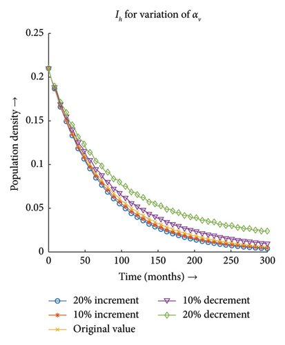
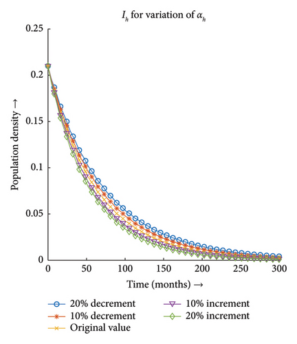
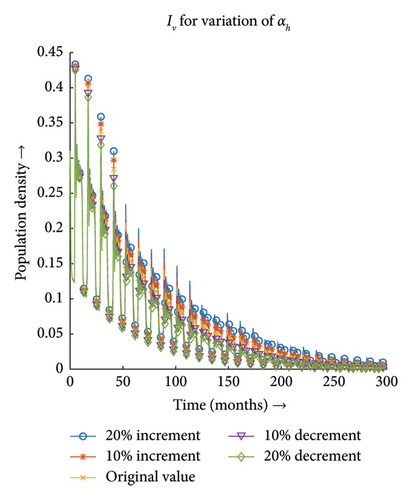
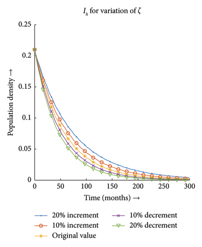
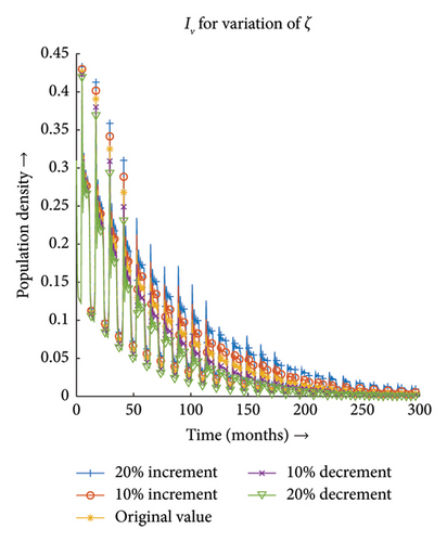
To understand the sensitivity of the aforementioned parameters on the dynamics of the model, we simulate the model numerically for controlled perturbation of the parameter values and visualize the effect on the infected compartments for both the host and vector side by side in the following discussion.

3.3.1. Effect of Gross Birth Rate or Per Capita Mortality Rate of Vector (α_v)

Figures 11(a) and 11(b) depict that the number of infections both in the case of vector and host increases with the decrease in the value of α_v and the same proportionality can be observed for the increment in the value of α_v. Hence, the infection dynamics in the heterogeneous population distribution are highly influenced by the deviation in the value of α_v.

3.3.2. Effect of Gross Birth Rate or Per Capita Mortality Rate of Host (α_h)

Figures 12(a) and 12(b) depict that the number of infections both in the case of vector and host decreases with the decrease in the value of α_h and the same proportionality can be observed for the increment in the value of α_h. Hence, the infection dynamics in the heterogeneous population distribution are highly influenced by the deviation in the value of α_h.

3.3.3. Effect of Recovery Rate of Host (ζ)

Figures 13(a) and 13(b) depict that the number of infections both in the case of vector and host decreases with the decrease in the value of ζ and the same proportionality can be observed for the increment in the value of ζ. Hence, the infection dynamics in the heterogeneous population distribution are highly influenced by the deviation in the value of ζ.

4. Discussion

This work has presented an explicit technique for using the linear operator method while avoiding algorithmic complexity, as well as findings that are consistent with earlier research [27, 45, 52, 59] and methodologies. The sensitivity analysis of the parameters in question has provided insight for public health officials on what to put the most weight on. It is evident that the most impactful parameter on the host dynamics is the gross birth rate/per capita mortality rate of the vector (α_v) followed by recovery rate (ζ), and for that of the vector, these are gross birth rate/per capita mortality rate of the vector (α_v) followed by the peak season infection rate of the vector (b_v). Hence, a strong emphasis must be placed on obstructing the growth of the vector population, defensive treatment of the infected, and curbing the number of interactions between the vector and host in order to flatten the curve in case of a raging epidemic. The assumptions used in this model constrained it; for example, the periodicity provided here was a square wave function, which may still be expanded to a much more generalized periodic function. The method proposed in this paper relies heavily on symbolic computation and hence can be a bit challenging to implement if the model is too complex. The simplification of this algorithm through theoretical advancement or to provide an alternate algorithm that elevates the problem of underperformance of the time-average method in the case of a nonautonomous system can be a potent avenue for research. There are aspects of the study that are looking for a technique that can offer the closed form of R₀, which helps with interpretability and analytic reasoning since the linear operator approach provides a numerical form of the fundamental reproduction number.

In the past we have seen that the worst known dengue outbreak in Bangladesh was in 2019, shown in Figure 2. A heat map comparison of the number of reported dengue cases during the years 2019, 2021, and 2022 is portrayed in Figures 14, 15, and 16, respectively. Each of the polygons in the heat map represents each division (first of order of administrative level in the country) of Bangladesh. We could not illustrate that of the year 2020 due to data unavailability.

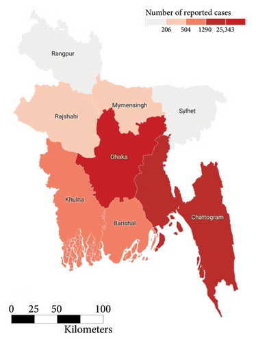
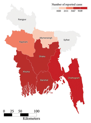
During the year 2019, the center and the southwestern regions of the country were the most affected regions followed by the southeastern. In the following year 2021, we saw uniform horizontal propagation from the center, southeastern, southwestern, and northwestern regions in the order of decreasing intensity with the most intensity in the center. Finally, in the year of 2022, we observe a similar pattern of infection distribution to that of 2019, with an increased intensity toward the southeastern region than the center.

Given the progressive level of environmental degradation, rapid urbanization and industrialization of the rural landscape, and increased adaptability of the Aedes mosquito to the increasingly harsh environment and devised countermeasures, we fear that the outbreaks of the coming years will be much more widespread and intense even than that of 2019. To tackle such multifacet, transdisciplinary challenges, we need models that are neither purely mathematical, which are interpretable, nor purely black box models like deep learning models but rather a hybrid of such models [60] and also threshold parameters that are much more data driven by construction [61]. These can be some avenues that require further research.

5. Conclusion

The amount of health and financial losses caused by viral illness on human civilization from the dawn of time is unfathomable. DENV is no different. DENV peaks in the second half of the year (May to September) in tropical areas across the world. In Bangladesh, a tropical nation in southern Asia, the following graphic depicts DENV cases and deaths.

DENV has shown a surge in cases and deaths not just in Bangladesh but also in nearly all of its infected regions. This has put afflicted countries’ governments and public health professionals in a difficult position. The merit of this paper is to provide a revamped algorithm to generate the BRN for the nonautonomous system. Unlike the time-average method, the linear operator method preserves the property of nonautonomousness of the system while deriving the BRN and can be used in much more complicated systems where the time-average method underperforms.

Ethics Statement

No consent is required to publish this manuscript.

Conflicts of Interest

The authors declare no conflicts of interest.

Author Contributions

M.K. and M.A.M. contributed to conceptualization; M.A.M. helped in methodology; M.A.M. and M.K. contributed to software; M.K. and S.C. helped in validation; M.A.M. and M.K. contributed to formal analysis; M.M.M. helped in investigation; S.C. and M.M.M. contributed to resources; M.A.M. helped in data curation; M.A.M. and M.K. prepared the original draft; M.M.M., S.C., and M.K. contributed to review and editing; and M.K. helped in supervision. All authors have read and agreed to the published version of the manuscript.

Funding

This project did not receive any funding.