Research on Local Fault Diagnosis of Rotary Vector Reducer Based on Motor Current Signature Analysis
Abstract
The rotary vector (RV) reducer, as a highly precise transmission mechanism, can lead to a series of consequential hazards when experiencing local faults. Conducting corresponding research on performance monitoring and fault diagnosis holds significant importance. In order to achieve higher diagnostic accuracy, better classification, prediction effect, and less use of sensors, this paper proposes a local fault diagnosis method of RV reducer based on Motor current signature analysis (MCSA). Firstly, the centre gear local fault electromechanical coupling model is created by combining the working principle of the servo motor, the working characteristics of the RV reducer, and the influencing factors of motor current. Then, according to the actual operating conditions of industrial robots (IRs), the corresponding experimental platform is designed and constructed, and current signals in four different modes are collected. Fast Fourier transform (FFT) is performed on the current signals to obtain frequency domain features, and the correctness of the local fault coupling model of the centre gear is experimentally verified. Finally, the time-domain statistical features, time–frequency domain features, and CNN features of servo-feedback current signals under different rotational speeds are extracted and used in the implementation of local fault diagnosis for the RV reducer, respectively. In this paper, it is confirmed that MCSA can be used for localized fault diagnosis of the RV reducer, and combined with a deep learning network, it can effectively predict the fault modes with an average accuracy of more than 96%.
1. Introduction
RV reducers have superior transmission precision and efficiency compared to ordinary reducers, making them widely utilized in fields such as IR, high-end CNC machine tools, and aviation equipment [1]. In recent years, with the rapid rise of intelligent manufacturing lines, IR technology has played a crucial role [2]. As an important supporting and transmission device, RV reducers significantly influence the precision control of IR systems, and their transmission performance can be used to evaluate the quality of IR systems. Currently, the monitoring of RV reducer states has become a hot topic in the industry, playing an irreplaceable role in reducing losses caused by reducer failures [3].
Due to the unique transmission principles and complex structures of RV reducers, previous research on RV reducers has mainly focused on multibody dynamics simulation analysis [4, 5], transmission characteristic analysis [6], and experimental testing [7]. Nowadays, researchers are turning to fault diagnosis research of RV reducers under various experimentally collected data [8, 9], especially using the method of vibration signal analysis. With the assistance of existing artificial intelligence algorithms, the fault degree of key components is identified, and the correlation between experimental data and fault modes is discussed [10, 11]. In 2018, Farajzadeh-Zanjani et al. [12] extracted features belonging to the time domain, the frequency domain, and the time–frequency domain of vibration signals and used them to classify bearing faults in induction motors. Long et al. [13] used the attitude sensor to collect the attitude data of the IR end to realize the fault diagnosis of the RV reducer, which took a lot of time and cost, and the classification effect was poor. Chen et al. [14] proposed a new method for fault diagnosis of RV reducers by combining the nonlinear output frequency response function (NOFRF) with convolutional neural network (CNN), aiming to address the problem of low accuracy in describing fault characteristics of vibration signals, which severely interferes with fault diagnosis accuracy. However, due to the interference of multiple factors, coupling, and external environmental changes [15, 16], the data collected by external sensors are often a combination of various complex signals, requiring more preprocessing analysis to achieve fault diagnosis.
With the development of computer technology, a large amount of useful information in the servo feedback current signal is mined out. MCSA was initially applied to monitor the state of the motor itself. [17–19]. Hussain et al.’s team [20, 21] has been using the combination of MCSA and deep learning (DL) to achieve fault detection and identification of internal structural parts of the motor, such as broken rotor bar and stator winding. In recent years, researchers have been conducted on various transmission chain devices such as harmonic reducers, planetary gears, and bearings based on MCSA [22–24]. Xu et al. [25] constructed an electromechanical coupling model for RV reducers’ bolt loosening and comprehensively evaluated experimental and simulation data, demonstrating the superiority of current signals. Lee et al. [26] extracted 27 feature information from the time domain, frequency domain, and time–frequency domain of servo motor feedback current for fault diagnosis of IR servo motors, validating the correlation coefficients between each feature signal. Yang et al. [27] utilized an improved driving algorithm to eliminate the interference of fundamental frequency and second harmonic in current signals during bearing fault diagnosis, thereby improving the accuracy of classification prediction. In addition, when extracting features using DL models, appropriate features can help researchers perform fault detection and identification of the corresponding rotating machinery [28]. The fault diagnosis method based on motor current is nonintrusive and does not require additional monitoring sensors, suggesting its potential for playing a more significant role in engineering applications in the future.
In summary, additional sensors are required for measurement when collecting transmission characteristics, attitude data, and vibration signals, and the fault diagnosis accuracy is not higher than that of current signals [29, 30]. The fault diagnosis technology for rotating machinery based on current signals has formed a relatively mature monitoring process, but the application of RV reducer fault diagnosis technology based on current signals is less common. The contributions of this study are as follows: (1) Combining the working principles of servo motors and simplifying RV reducers faults into stiffness changes, an electromechanical coupling model of local faults in the servo transmission chain was established. (2) In order to simulate the load change, an experimental platform that is capable of emulating the IR working mechanism has been designed and constructed. The correctness of the local fault coupling model of the centre gear is verified by the spectrum analysis experiment of the collected current signal. (3) Extracting time-domain statistical features, time–frequency domain features, and CNN features from the collected current signals, conducting dimensionality reduction clustering and classification prediction, and achieving local fault diagnosis of RV reducers, demonstrating the feasibility of MCSA in local fault diagnosis.
2. Electromechanical Coupling Model
2.1. Analysis of Local Faults in the Centre Gear
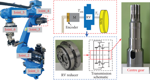
Serial-type industrial robot joint servo systems are primarily composed of permanent magnet synchronous motors (PMSM), RV reducers, and mechanical arms, as shown in Figure 1. In the figure, Tem and Tl represent the servo motor output torque and load torque, respectively. The following text will use the RV-20E reducer as an example to establish an electromechanical coupling model under the local fault mode of the centre gear.
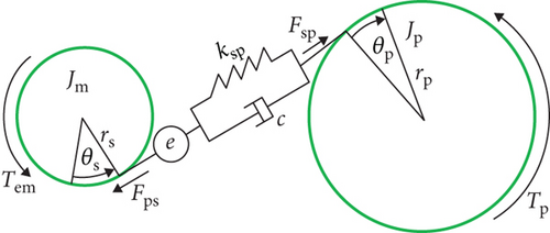
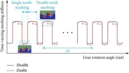
In this case, the selected planetary gear transmission has a meshing factor greater than 1, leading to both single-tooth meshing and double-teeth meshing during actual transmission. This results in a periodic variation of meshing stiffness with rotation angle, resembling a square wave. When the localized fault occurs in any gear transmission, it significantly impacts the meshing stiffness, as depicted in Figure 3. Each time the faulty gear engages in meshing, torque fluctuation occurs, causing the transmission error e to become uncertain, resulting in corresponding pulse signals in the input torque.
2.2. Principle of Operation of Servo Motors
The PMSM is utilized as the power source for the test setup in the paper, where the amplitude, frequency, and phase of the torque current are adjustable. By varying the frequency of the stator winding current, the motor rotor can be accelerated or decelerated to balance power fluctuations caused by changes in the load, thereby reducing disturbances to the system. The physical model of the PMSM is illustrated in Figure 4, where θm represents the rotor mechanical angular displacement (output angle). In motor control, the electrical displacement angle θr is commonly used for calculations, where θm and θr satisfy θm = θr/P, with P denoting the number of motor pole pairs.
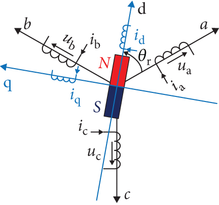
Where Ld represents the d-axis inductance, Lq represents the q-axis inductance, Φf represents the magnetic flux generated by the rotor excitation poles.
The servo motor output torque is related to angular velocity, angular acceleration, and load torque, and it is very challenging to simulate the current signals under each localized fault condition during actual operation. Therefore, when using current signals to monitor the operating conditions of the RV reducer, a deeper analysis of its drive chain system is required.
2.3. Centre Gear Local Fault–Coupling Model
2.3.1. The Characteristics of Electromagnetic Torque
2.3.2. The Characteristics of Motor Current
3. Data Acquisition and Model Validation
3.1. Testing Platform
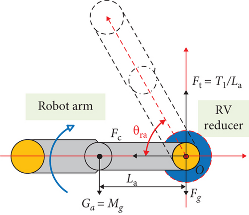
Taking IR Joint 3 as an example, the work is similar to a rod rotating around the end point, and the 4–6 axes are viewed as a whole M for force analysis and found that the RV reducer is subjected to time-varying torque. To approximate the torque experienced by the reducer to the actual situation, a load is added to the end effector, and the fluctuation of torque during motion is ignored. Thus, the reducer only experiences the gravitational force Ga = Mg from Axes 4–6, as shown in the force analysis in Figure 5. Here, O represents the centroid of the simplified model, Fc is the centrifugal force exerted on the RV reducer, Fg is its own weight, and the tangential stress generated by the load is Ft = Tl/La, where g and La represent the gravitational acceleration (9.8 m/s2), the distance from the centroid to the centre of the reducer when in the horizontal position, respectively.
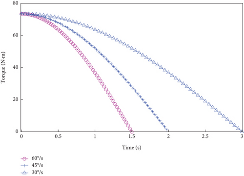
To enable rapid and precise monitoring of the RV reducer with high reliability and the ability to conduct comprehensive performance evaluations even under complex conditions, a magnetic powder brake is utilized to simulate the dynamic torque variations depicted in Figure 6. Corresponding loading experiments are conducted to acquire experimental data under simulated real-world conditions. Firstly, according to the experimental requirements, a servo system with a 23-bit absolute encoder and high-speed control accuracy is selected as the input device. In order to better simulate the load torque, a magnetic powder brake with a controllable loading torque and a maximum torque of 400 N·m is used. Some key parameters of the test platform device are shown in Table 1.
| Measurement device | Models | Key parameters (partial) | |
|---|---|---|---|
| Servo motor |
|
Nominal output/(kW) | 0.75 |
| Rated torque/(N·m) | 2.39 | ||
| Rated speed/(rpm) | 3000 | ||
| Torque/speed sensor | HY-5005 | Sampling range/(N·m) | 0–400 |
| Maximum speed/(rpm) | 3000 | ||
| Measurement accuracy | ± 0.2% | ||
| Magnetic particle brake | CZ-40 | Torque range/(N·m) | 0–400 |
| Excitation current/(A) | 0–3 | ||
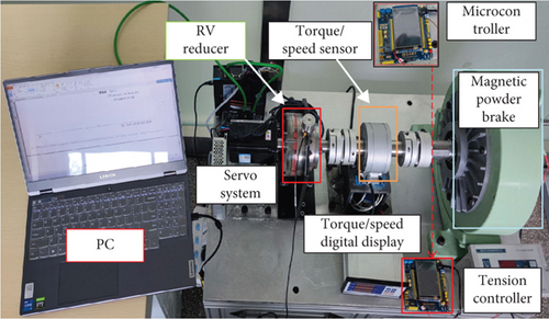
In addition to the measurement device mentioned above, this testing platform also requires some auxiliary equipment, such as a workbench, elastic couplings, and sensor support fixtures. According to research requirements, an open-loop control structure is adopted to build the corresponding testing platform. The installation positions and distribution of each device are shown in Figure 7.
3.2. Fault Setting and Data Acquisition
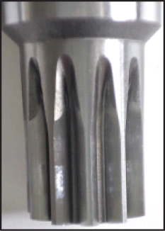
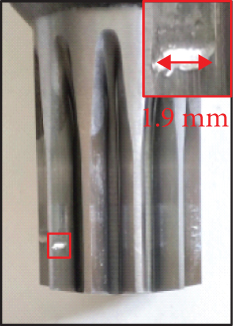
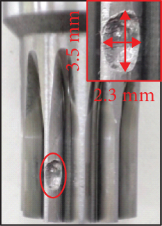
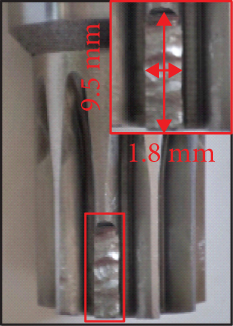
In this experiment, localized faults only in the centre gear are considered. The different sizes of defects are introduced on one of the teeth, as shown in Figure 8, which simulate common gear faults such as pitting, spalling, and tooth breakage, respectively. Among these, the severity of pitting fault is lower than that of spalling, while tooth breakage represents the most severe fault mode. As the operational state of the reducer is significantly affected by the rotational speed, the theoretical output speeds of the servo motors correspond to the output speeds ωrv of the RV reducer. The magnetic powder brake is used to simulate the corresponding load conditions, and three loading experiments are carried out in each mode. A total of 12 sets of experimental data are obtained.
After the experimental validation, to avoid excessively high sampling frequencies, which could compromise the quality of low-frequency signals, the sampling frequency is set to 1 kHz following the Nyquist sampling theorem. And get real-time feedback on the current signal of the servo motor by upper computer software. The collected data is regarded as a sample with 4096 data points, and 200 samples are extracted from each group. A total of 819,200 data points are used. The actual current signal (a certain sample sequence) is shown in Figure 9.

Comparing the above time-domain signals, it is found that the trends of the current signals are cyclic with the rotational speed and attitude of the IR joints in Figure 9. The relative currents increase when the load torque becomes larger and do not change significantly for the same operating mode and different rotational speeds. Except for the occurrence of more pulses in the tooth breakage fault mode, the time-domain signals in the pitting and spalling conditions are similar to those in the healthy state, making it difficult to classify the severity of the faults.
3.3. Fault Coupling Model Experimental Verification
Combining with the working principle of the servo motor, the theoretical output speed n1 = 60f/P is obtained, where f is the pulse frequency output by the servo driver and P is the number of pole pairs of the motor. According to the transmission principle of the RV reducer [33, 34], when the needle gear housing is fixed, the working frequency of the key components of the RV reducer and the meshing frequency of the two-stage transmission can be obtained. The specific calculation formulas and related parameter attributes are shown in Table 2.
| Title | Formulas | Properties |
|---|---|---|
| Fundamental frequency of servo motor/fe | fe = (n1 · P)/60 | p = 5 |
| Frequency of centre gear rotation/f1 | f1 = n1/60 | / |
| Frequency of planetary gear (crankshaft) rotation/f2 | f2 = (f1 · Z5)/i | Z5 = 39; i = 121 |
| Frequency of planetary support racks rotation/f3 | f3 = f1/i | / |
| Frequency of primary engagement drive/fsp | fsp = (f1 · Z2 · Z4)/i | Z2 = 33; Z4 = 40 |
| Frequency of secondary engagement drive/fcs | fcs = (f1 · Z4 · Z5)/i | / |
- Note: Z2 represents the number of teeth on the planetary gear, Z4 represents the number of teeth on the pinion gear, and Z5 represents the number of teeth on the cycloid gear.
Then, the theoretical formula in Table 2 is used to calculate the RV reducer’s corresponding rotation frequency and meshing frequency at three speeds. The specific theoretical calculation values are shown in Table 3.
| Output speed/(°/s) | Frequencies/(Hz) | |||||
|---|---|---|---|---|---|---|
| fe | f1 | f2 | f3 | fsp | fcs | |
| 30 | 50.42 | 10.08 | 3.25 | 0.083 | 109.96 | 129.96 |
| 45 | 75.625 | 15.125 | 4.875 | 0.125 | 165 | 195 |
| 60 | 100.83 | 20.17 | 6.5 | 0.167 | 220.04 | 260.04 |
Finally, we perform the fast Fourier transform analysis on the current signals in Figure 9 to obtain the spectrum plot as shown in Figure 10.

In Figure 10, the corresponding rotation frequency and meshing frequency in Table 2 are marked, where labels (a–d) correspond to the previous text. Combining the theoretical calculation results from Table 3 with the spectrum results in Figure 9, it can be observed that under different operating conditions, the fundamental frequency of the servo motor (fe), the rotation frequencies of the RV reducer (f1, f2, f3), and the meshing frequencies (fsp, fcs) can be effectively extracted. In addition to these frequencies, significant amplitudes are also observed at fe ± f1, |fe ± fsp|, and |fe ± fcs| frequencies (where f2 and f3 values are too small, and fe ± f2, fe ± f3 amplitudes are not significant). From the perspective of experimental analysis, the correctness of the electromechanical coupling model in the case of local failure of the centre gear is verified. At the same time, it is proved that the servo feedback current signal can be used for local fault diagnosis of the RV reducer. Due to the dead zone effect in the servo motor drive system, there will be significant amplitudes near 5 times the motor fundamental frequency. Comparing the spectrum plots of the four states of the centre gear, it is observed that apart from the noticeable continuous f1 sidebands in the case of tooth breakage faults, sidebands are not significant in the case of pitting and spalling fault modes, making it difficult to assess the severity of the faults.
4. Results and Discussion
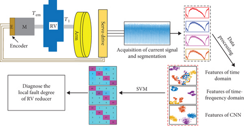
When the IR is running with load, there are multicondition coupling effects, and the rotational motion is extremely unfavorable to the installation of the sensor. With the development of servo systems, their feedback information has become increasingly widespread in practical applications, not limited to motion accuracy control but also playing a proactive role in monitoring the status of their transmission chains. MCSA is a typical method with low cost and simplicity. The method proposed in the article for local fault diagnosis of the RV reducer is shown in the flowchart in Figure 11. Firstly, the current signal feedback from the servo motor is obtained through upper computer software, and the samples are divided according to the data division described earlier. Then, time-domain statistical features, frequency-domain statistical features, and CNN features of the current signal are extracted. Finally, these features are input into a support vector machine model to identify the degree of local faults in the RV reducer under different speed conditions.
4.1. Based on Time-Domain Statistical Features
To better illustrate the impact of local faults in the RV reducer on the servo feedback current signal, 10 statistical features t1 − t10 are extracted from the current signal, as shown in Table 4.
| Features | Formula |
|---|---|
| Peak-to-peak values | t1 = |xmax − xmin| |
| Mean | |
| Variance | |
| Root mean square | |
| Square root amplitude | |
| Kurtosis | |
| Pulse factor | t7 = t1/2t2 |
| Margin factor | t8 = t1/2t5 |
| Peak factor | t9 = t1/2t4 |
| Waveform factor |
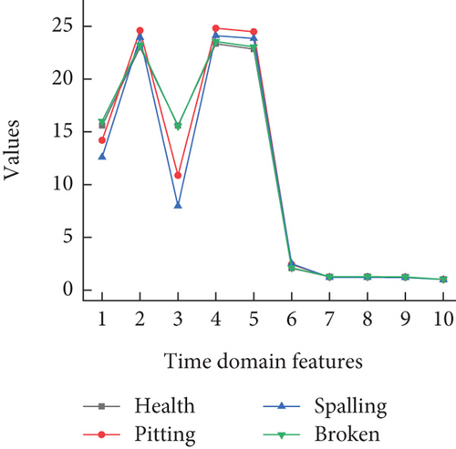
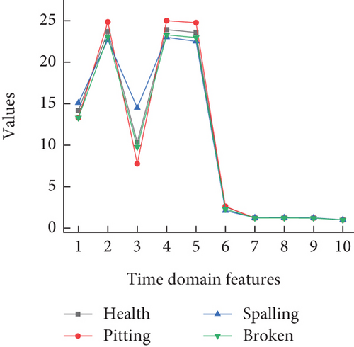
Using the calculation formulas in Table 4 to determine the characteristics of the data in Figure 9, obtain the time-domain features under three different rotational speed conditions as shown in Figure 11.
Based on the distribution of time-domain features in Figure 12, it can be observed that the trend of feature changes is roughly similar under different rotational speed conditions. The distinct differences in features t1 − t5 are advantageous for classifying local faults in the RV reducer, while features t6 − t10 are less affected by faults. However, due to the interference of the RV reducer’s fluctuation factors, there is an overlapping phenomenon in significantly changing features. Next, the t-SNE algorithm is used to nonlinearly map high-dimensional data to a representational space to achieve feature dimension reduction. This allows for better visualization and analysis of sample features, reducing information redundancy between high-dimensional feature vectors and improving classification efficiency and accuracy. The feature data obtained after dimension reduction are assigned to the same quantified space, resulting in a visualization analysis of time-domain features, as shown in Figure 13.

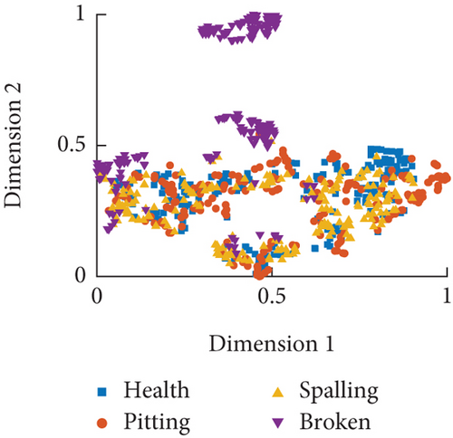
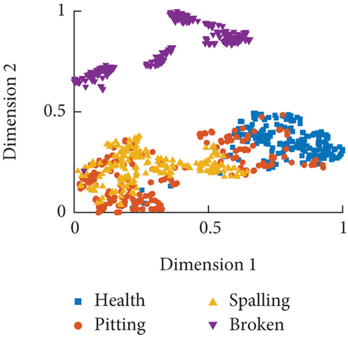
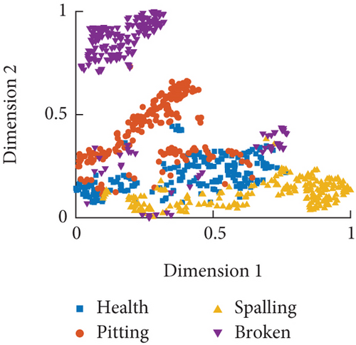
From the dimensionality reduction results in Figure 13, it can be observed that time-domain features are most sensitive to gear tooth faults, but their effectiveness in recognizing the other three fault modes is poor, especially at a speed of 30°/s where the classification performance is the worst. A comparison of the three classification results indicates that the research on local fault diagnosis of RV reducers using current signal time-domain features poses a challenge.
4.2. Based on Time–Frequency Domain Features
From the spectral analysis results in Figure 10, it can be observed that frequency-domain signals are not conducive to achieving multimode recognition of RV reducers. And it is not introduced repeatedly in this section. Next, the time–frequency domain statistical features of the above signals are extracted for RV reducer fault diagnosis and identification. Wavelet packet decomposition (WPD) can effectively overcome the key difficulty of indistinct representation of current signals and spectral aliasing. It also enhances the accuracy of classification prediction. WPD maps one-dimensional time-domain current signals to two-dimensional time–frequency domain signals. It decomposes the signal into high-frequency and low-frequency components, effectively improving time–frequency resolution while extracting more crucial feature information. The structure of WPD is illustrated in Figure 14.
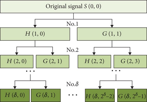
The experimental results show that optimal results can be obtained when the number of decomposition layers is 4. The energy values of 16 sub-bands from high frequency to low frequency in the fourth layer are extracted as the eigenvalues needed in this paper. Then, the “energy-fault diagnosis” method is established. The time–frequency domain features of the data in Figure 9 are calculated, and the time–frequency domain characteristics under three different speed conditions are obtained, as shown in Figure 15 (disregarding interference from high-frequency components, taking w1 − w14 as 14 feature values).
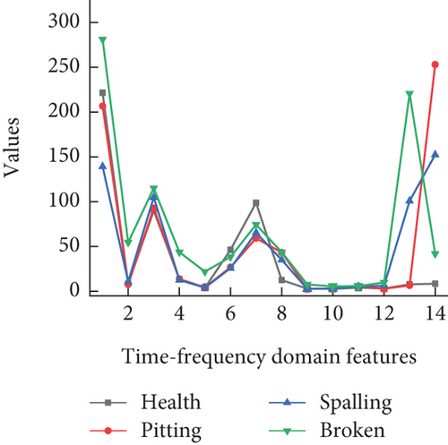
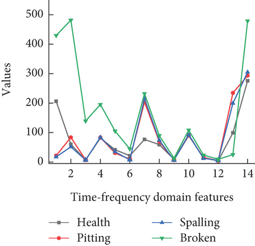
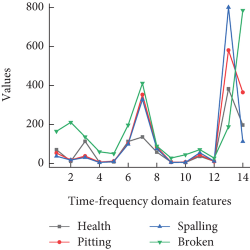
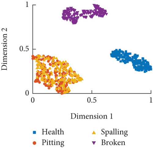
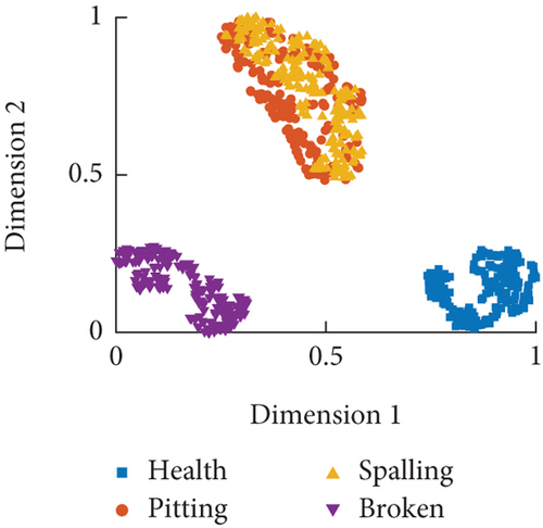
From the distribution of time–frequency domain features in Figure 15, it can be observed that most features can effectively distinguish between the four operating modes. Particularly, there is significant discrimination between the healthy and tooth fault modes, while the discrimination is less pronounced for the pitting and spalling modes, which hinders fault diagnosis. The visualization analysis of the time–frequency domain features after dimensionality reduction is shown in Figure 16. The dimensionality reduction results correspond to the feature distribution, effectively classifying between the healthy and tooth fault modes but showing poor classification performance for the pitting and spalling faults. Even under a speed condition of 60°/s, all four operating modes can be effectively distinguished, although the discrimination between pitting and spalling faults is relatively close.

4.3. Based on CNN Features
After analyzing the time domain, frequency domain, and time–frequency domain features above, it is evident that employing simple feature extraction methods leads to results that are not sufficiently clear or accurate. With the advancement of computer technology, DL has been widely applied in the extraction of state features and classification prediction of various industrial equipment [35]. Next, CNNs will be utilized to learn and extract deeper-level features from the local relationships within the data.
CNN is a deep feedforward neural network with the characteristics of parameter sharing and local perception. CNN is generally composed of the input layer, convolution layer, activation layer, pooling layer, and fully connected layer. The specific network structure is shown in Table 5.
| Layers | Layer | Activation function | Convolution kernel/step | Number of convolution kernels | Input (output) dimensions |
|---|---|---|---|---|---|
| 1 | Input layer | / | / | / | 1@1 × 4096 |
| 2 | Convolutional-1 | ReLU | 1 × 7, 1 | 8 | 8@1 × 4090 |
| 3 | MaxPooling-1 | / | 1 × 3, 2 | 8 | 8@1 × 2044 |
| 4 | Convolutional-2 | ReLU | 1 × 5, 1 | 8 | 8@1 × 2040 |
| 5 | MaxPooling-2 | / | 1 × 3, 2 | 8 | 8@1 × 10¹⁹ |
| 6 | Convolutional-3 | ReLU | 1 × 3, 1 | 16 | 16@1 × 10¹⁷ |
| 7 | MaxPooling-3 | / | 1 × 3, 2 | 16 | 16@1 × 508 |
| 8 | Output layer (FC) | / | / | / | 32@1 × 1 |
The initial learning rate of the learning model is set to 0.005, and it decreases by 50% every 10 iterations, for a total of 30 iterations. The data extracted from the fully connected layer is considered as the sample features, and the visualization results obtained after dimensionality reduction using t-SNE are shown in Figure 17.
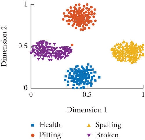
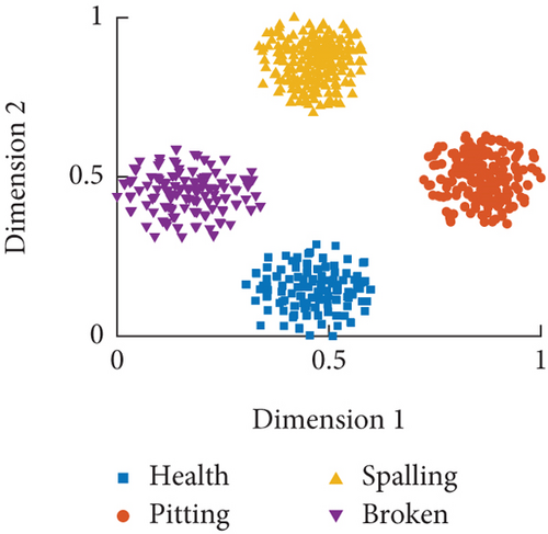
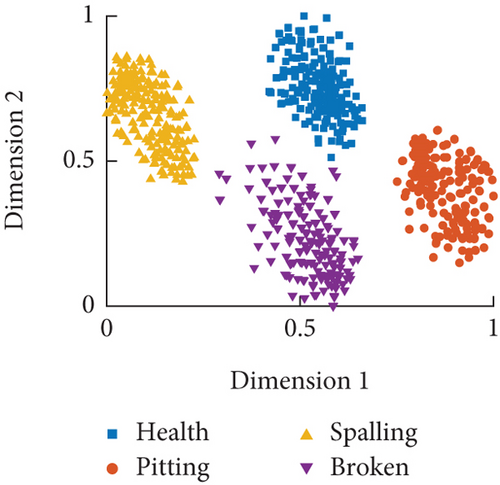
From the distribution results in Figure 17, it can be observed that after CNNs feature extraction and visualization analysis, the sample data under different fault modes demonstrate good recognition performance for minor faults such as pitting and spalling across various speed conditions. As the severity of faults increases, the feature information of the sample data tends to diverge. Particularly in Figure 17(c), the dispersion is significant for the tooth fault mode. This divergence may affect further classification prediction, indicating that when RV reducers experience severe faults, the collected information becomes disordered and uncontrollable.
4.4. Comparative Analysis of Prediction Results
Generally, classification accuracy is used as an assessment standard of the methods. However, in order to explore better feature extraction methods, a confusion matrix is introduced in the paper. The relationship between the true category of the samples and the classification result is described by the confusion matrix to present the assessment standard of model performance. The confusion matrix is shown in Table 6.
| Real value | Classification value | |
|---|---|---|
| Positive | Negative | |
| Positive | True positive (TP) | False positive (FN) |
| Negative | False positive (FP) | True positive (TN) |
- Note: TP is the number of positive cases predicted to be positive, FP is the number of negative cases predicted to be positive, FN is the number of positive cases predicted to be negative, and TN is the number of negative cases predicted to be negative.
The extracted sample features are then classified using SVM. The features are labeled according to their corresponding failure modes and the feature matrix is divided into a training set and a test set, where the training set is used for model training and the test set is used for model accuracy testing. The training set and test set are 70% and 30%, respectively, and the computation is repeated 10 times, respectively. The resulting confusion matrix under three different features is shown in Figure 18.
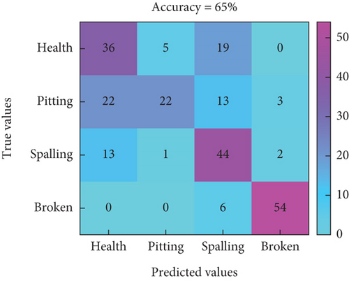
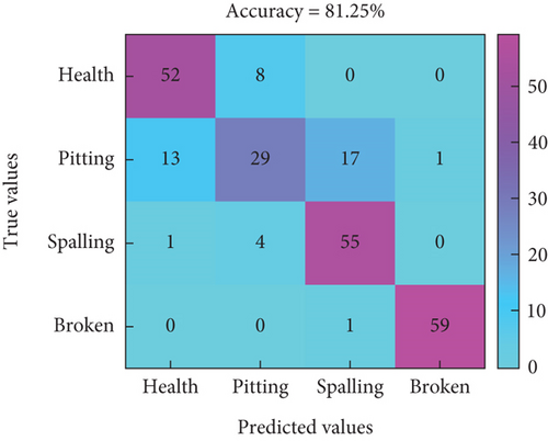
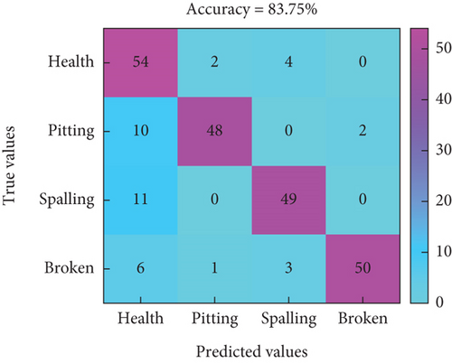
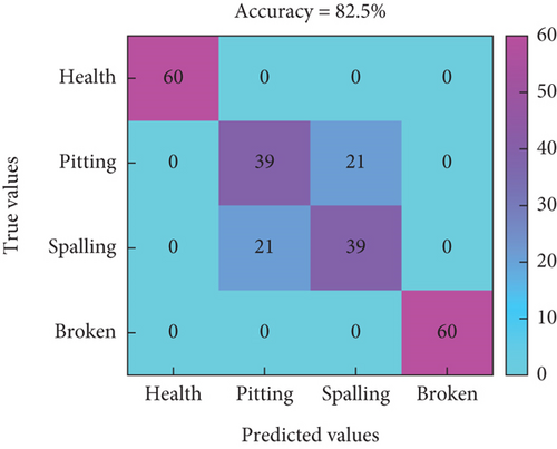

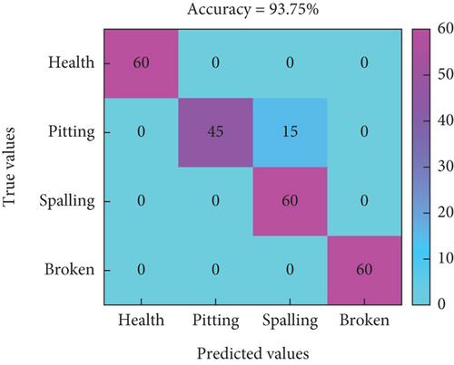

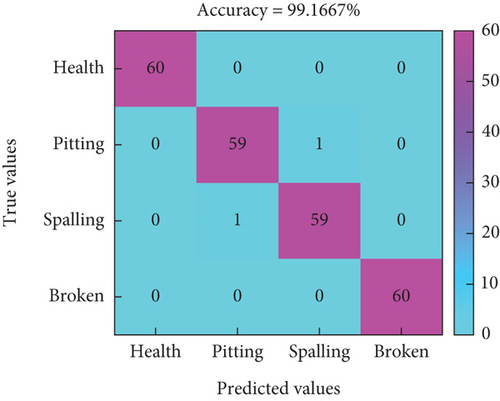
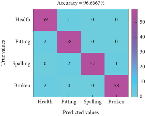
In Figure 18, the horizontal axis represents the predicted labels for different modes, while the vertical axis represents the true labels for fault modes. Figures 18(a), 18(b), and 18(c) represent the classification prediction results for three different speeds under time-domain features, and the highest accuracy rate is only 83.75%. Figures 18(d), 18(e), and 18(f) represent the classification prediction results for three different speeds under time–frequency domain features, with an overall accuracy rate higher than 82.5%. In this feature mode, there is potential for local fault diagnosis of RV reducers. Figures 18(g), 18(h), and 18(i) represent the classification prediction results for three different speeds under CNN features, with an average accuracy rate higher than 96%.
The results of the distribution of the confusion matrix in Figure 18 were solved to obtain the mean values of Pre, Rec, and F1 for three different feature extraction methods, as shown in Figure 19.
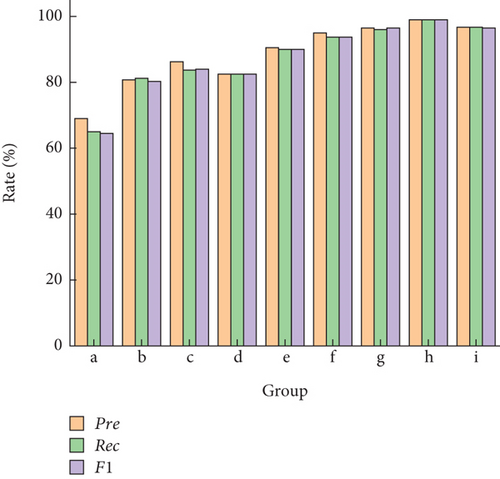
In Figure 19, these performance metrics Pre, Rec, and F1 perform worst at low rotational speed using time domain statistical features for classification. And it can be seen that rotational speed has a certain influence on the assessment indicators from label (d). Under CNN features, with an average Pre, Rec, and F1 rate higher than 96%. As can be seen from the distribution of results in Figures 18 and 19, using CNN features or other complex feature extraction methods holds the most promising application prospects for local fault diagnosis of RV reducers.
5. Conclusions
In this study, we first established the model and analysis of the servo transmission chain system, identifying theoretical factors influencing current characteristics. Through experimental validation, we confirmed the correctness of the fault coupling model, meanwhile providing theoretical support for using Motor Current Signature Analysis (MCSA) in RV reducer fault diagnosis research. During FFT analysis of the collected current signals, it was found that fault characteristic frequencies for minor fault modes such as pitting and spalling were not distinct, which hindered RV reducer performance assessment. Therefore, it was necessary to extract time domain, time–frequency domain, and CNN features. The research results indicate that using SVM for classification prediction based on extracted time-domain statistical features and time–frequency domain features resulted in relatively low average accuracy rates. These methods were also significantly influenced by speed conditions, with average accuracy rate differences of 18.75% and 11.25% under three different speeds, indicating substantial variability and limitations in fault severity recognition and monitoring. At the same time, under CNN feature conditions, the mean values of Pre, Rec, and F1 show the best results, and the average fault diagnosis accuracy rate exceeded 96%, with minimal average accuracy rate differences of only 2.92% under three different speeds. Therefore, utilizing CNN features for local fault severity recognition in RV reducers holds greater research value. These findings provide insights for “sensor-less” performance monitoring and fault diagnosis of RV reducers in IR, demonstrating the larger development and application potential of MCSA in servo transmission device condition monitoring.
Conflicts of Interest
The authors declare no conflicts of interest.
Funding
This research has been supported by Qinghai Province “Kunlun Talents High-end Innovation and Entrepreneurship Talents” Plan Project (grant no. K9923194), Qinghai University Intelligent Manufacturing Engineering Innovation Experimental Class Construction Project (grant no. RCPY-2021-04), and the Ministry of China Education’s Industry-University-Research Collaborative Education Project (grant no. 202102108040).
Acknowledgments
This research has been supported by Qinghai Province “Kunlun Talents High-end Innovation and Entrepreneurship Talents” Plan Project (grant no. K9923194), Qinghai University Intelligent Manufacturing Engineering Innovation Experimental Class Construction Project (grant no. RCPY-2021-04), and the Ministry of China Education’s Industry-University-Research Collaborative Education Project (grant no. 202102108040).
Open Research
Data Availability Statement
The data used to support the findings of this study are available from the corresponding author upon request.


