The differential transformation method (DTM) is one of the best methods easily applied to linear and nonlinear difference equations with random coefficients. In this study, we apply the theorems related to the DTM to the given examples and investigate the behaviour of the approximate analytical solutions. The expected value, variance, coefficient of variation, and confidence intervals of the solutions of random difference equations obtained from discrete probability distributions such as uniform, geometric, Poisson, and binomial distributions will be calculated. Maple and MATLAB software packages are used to plot the solution graphs and also to interpret the solution behaviour.

1. Introduction

The differential transformation method was introduced by Zhou in 1986 for solving linear and nonlinear problems involving electrical circuit problems [1]. The differential transformation method is a numerical technique based on the Taylor series expansion, which forms an analytical solution in polynomial form, and from this technique, the exact solutions for the differential or the integrodifferential equation are obtained [2]. Abbasov and Bahadir and Abdel and Hassan [3, 4] used the differential transformation method to obtain approximate solutions of linear and nonlinear equations related to engineering problems and observed that the numerical results were in good agreement with analytical solutions. In addition, the operations performed are possible to solve linear or nonlinear problems of difference equations.

The theory of difference equations, which has attracted much attention in the last few years, is rapidly advancing in a wide range of applications. While random dynamical systems can mathematically express an equation, events observed in nature represent a dynamical process. These systems are time-varying systems. Difference equations arise in the discretisation methods of differential equations. Difference equations have many applications in many fields of mathematics and science such as economics, biology, signal processing, computer engineering, genetics, medicine, ecology, and fixed point theory [5]. Difference equations, which have applications in various branches of science, lead to many mathematical analyses. The method we have developed here is applied to obtain the solution of initial value problems, difference equations, and boundary value problems. With the rapid progress of science, complex nonlinear difference equations allow us to analyse more easily [5–8].

In this article, the solution of difference equations is calculated with the help of the differential transformation method. Section 2 contains definitions and fundamental theorems with DTM. In Section 3, the basic technique of difference equations is given. In Section 4, brief information about discrete probability distributions is given, and in Section 5, the results are calculated by applying them to numerical examples.

2. Differential Transformation Method

The differential transformation of a function y(x) is defined as follows:

(1)

Here, y(x) is the original function and Y(k) is the transformed function. The inverse of the differential transformation is defined as follows:

(2)

The theorems obtained from Equations (1) and (2) are given below:

Theorem 1. If y(x) = f(x) ± g(x), then Y(k) = F(k) ± G(k).

Theorem 2. If y(x) = cf(x), then Y(k) = cG(k), where c is a fixed number.

Theorem 3. If y(x) = dⁿg(x)/dxⁿ, then Y(k) = ((k + n)! /k!)G(k + n).

Theorem 4. If y(x) = f(x)g(x), then .

Theorem 5. If y(x) = xⁿ, then Y(k) = δ(k − n), where

Theorem 6. If y(x) = f₁(x)f₂(x) ⋯ f_n−1(x)f_n(x), then

( )

Theorem 7. If y(x) = f(x + a), then for N⟶∞.

Proof 1. Using the definition of DTM in Equation (2),

( )

By combining these given series

( )

And in the transformation definition in Equation (2), if Y(k) is written as follows:

( )

Theorem 8. If y(x) = f₁(x + a₁)f₂(x + a₂), where

for N⟶∞.

Proof 2. Let C₁(k) be the differential transform of f₁(x + a) and C₂(k) be the differential transform of f₂(x + a) at x = x₀. Using Theorem 4, the differential transformation of y(x) is obtained as follows:

( )

And from Theorem 7,

and

( )

Using values

( )

Theorem 9. If y(x) = f₁(x + a₁)f₂(x + a₂) ⋯ f_n−1(x + a_n−1)f_n(x + a_n), then

( )

Proof 3. Let C_i(k) be the differential transform of f_i(x + a_i) at x = x₀ for i = 1, 2, 3, ⋯, n. Then, using Theorem 6, we obtain the differential transformation of y(x) as follows:

( )

And using Theorem 7,

( )

By utilising these values,

( )

In general,

( )

Theorem 10. If

( )

Proof 4. Let C_i(k) be the differential transform of g_i(x + a_i) for i = 1, 2, 3, ⋯, n and i = 1, 2, 3, ⋯, m. Let h_j(x)H_j(k) for x = x₀. Then, using Theorem 6, we obtain the differential transformation of y(x) as follows:

( )

Using Theorem 7,

( )

By utilising these values,

( )

In general,

( )

Theorems 1–5 are well known in the literature, and they cannot be proved here, and the proof of Theorem 6 is available in [9].

3. Solution Techniques for Difference Equation

Consider the following constituted difference equation [10]:

(3)

With conditions

(4)

From Theorems 7–10, it can be seen that the transformation of Equation (3) gives an expression of the following form:

(5)

where N is a large enough integer. Then the transformation of the BCs in Equation (4) using Equation (2) can be shown in the following:

(6)

The solution of difference Equation (3) requires the solution of the coefficients F(0), F(1), ⋯, F(N), so we must have N + 1 equations for N + 1 unknowns. From Equation (6), we have n equations given as BC, and the remaining N − n + 1 equations must be obtained from Equation (5) for k = 0, 1, ⋯, N − n. If Equation (3) is linear, the problem is simply to take the inverse of the coefficient matrix and multiply it by the right-hand side of Equation (5), but if Equation (3) is not linear, the set of equations must be solved by one, for example, Newton’s method. The differential transformation method has been applied to chaotic models, Volterra and Fredholm integral equations, fractional order equations, and partial differential equations and has been used to obtain very useful solutions [11–17].

4. Probability Distributions in Discrete Time

Definitions of some commonly used concepts in probability are provided in this section [18].

4.1. Discrete Uniform Distribution

Definition 1. Assume that k is an integer bit. The discrete uniform chance variable is the term used to describe a random variable with probability function.

( )

Theorem 11. When has a uniform distribution that is discrete, then

4.2. Bernoulli Distribution

Definition 2. An random variable is referred to as a Bernoulli random variable if there are only two possible outcomes. The probability mass function is used to derive Bernoulli variables.

( )

Theorem 12. If has a Bernoulli distribution,

4.3. Binomial Distribution

Definition 3. Let the random variable be the total number of people who passed n independent Bernoulli trials. The probability of failure for a particular experiment is , whereas the likelihood of success is represented by . The probability function of the binomial random variable is as follows:

( )

The calculation of consecutive binomial probabilities is as follows:

( )

Theorem 13. If has a binomial distribution,

4.4. Geometric Distribution

Definition 4. A geometric random variable is the number of experiments conducted in a Bernoulli experiment repeated n times successively in order to get the first intended result (success or failed). This variable’s distribution is known as the geometric distribution, and its probability function is the geometric random variable , with a single experiment’s probability of success being and of unsuccessfulness being .

( )

Theorem 14. If has a geometric distribution,

4.5. Poisson Distribution

Definition 5. . The Taylor expansion of the function e^y and the probability function gives :

( )

Theorem 15. If has a Poisson distribution,

5. Numerical Results

Example 1. Consider the following linear difference equation with variable coefficients:

(7)

Let us examine the solution behaviour of the equation with A ~ U(α = 2, β = 4) uniformly distributed random variables and B ~ Be(p = 2/3, q = 1/3) Bernoulli distributed random variables.

The initial conditions are as follows:

(8)

Using Theorems 5, 7, and 10, the differential transformation method of Equation (7) is obtained as follows:

(9)

where N is a sufficiently large integer. The BCs in Equation (8) can be transformed at x₀ = 0 as follows:

(10)

Taking N = 4, the following system of equations can be obtained from Equation (9) for k = 0, 1, 2.

(11)

From the system of Equation (11), we obtain the following:

(12)

Then, using the inverse transformation rule in Equation (2), we obtain

(13)

where α = x^′(0) = X(1) missing BC. The numerical value of α is obtained from the second part of Equation (10) as α = 16B/37 − A. Then, Equation (13) becomes

(14)

It can be seen from Equations (13) and (14) that the coefficients of the series vary with N, which is a consequence of the implicit behaviour of the solution technique. With N = 4, comparative numerical results and the exact solution of x(n) = B2ⁿ − (A + B)n + A are obtained.

For higher order moments of random variables, the approximate expected value, variance, and coefficient of variation (CV) are calculated. For a uniformly distributed random variable X

A ~ U(α, β) and B ~ Be(p, q) moment extraction function

( )

Therefore, the first moment and variance of the random variable X are as follows:

( )

Let us find the probability characteristics of the solution obtained in Equation (14). Firstly, the expected value is as follows:

( )

The variance is as follows:

( )

Let A, B ~ U(α = 4, β = 2) be the parameters. The numerical characteristics of the approximate solutions of the obtained random linear difference equation are obtained by calculating as follows:

( )

is obtained and variance,

( )

CV is calculated as 100 × std(X(n))/E(X(n)) by definition. The CV is

( )

is obtained.

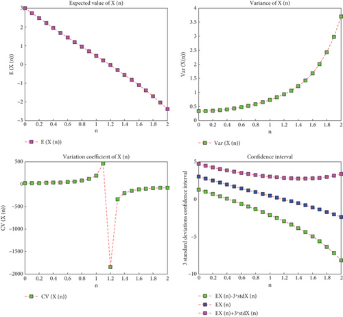
Figure 1 provides the solutions for the expected value, variance, CV, and confidence interval of the n ∈ [0, 2] distribution. It can be noted that the mean value lowers as the variability increases, indicating an increase in random fluctuations.

Details are in the caption following the image — **Figure 1**
Open in figure viewer PowerPoint

Plots of expected value, variance, coefficient of variation, and confidence intervals obtained from random DTM transformation of Equation (14).

Table 1 provides the expected value, variance, and confidence interval for K = 3 values. As can be observed, the outcomes for values of n ∈ [0, 1] are obtained in a manner akin to that of the case with uniform and Bernoulli parameters.

Example 2. Consider the following linear difference equation with variable coefficients:

(15)

Table 1. Table for the expectation value, variance, coefficient of variation, and 99% confidence interval.

n	E[X(n)]	Var[X(n)]	CV[X(n)]	E[X(n)] − 3Std[X(n)]	E[X(n)] + 3Std[X(n)]
0	3	1/3	19.245008	1.267949	4.732050
0.1	2.729993	0.337082	21.267020	0.988228	4.471758
0.2	2.462796	0.348337	23.964692	0.692191	4.233400
0.3	2.198949	0.367122	27.554344	0.381231	4.016668
0.4	1.938760	0.393487	32.355007	0.569021	3.820618
0.5	1.682296	0.427534	38.867182	−0.279287	3.643880
0.6	1.429391	0.469448	47.933910	−0.626098	3.484882
0.7	1.179643	0.519561	61.103760	−0.982775	3.342062
0.8	0.932410	0.578437	81.568281	−1.349242	3.342062
0.9	0.686817	0.647008	117.11531	−1.726287	3.099922
1	0.441752	0.726756	192.98157	−2.115748	2.999252

Let us examine the solution behaviour of the equation for random variables with geometric distribution A ~ G(p = 3/4, q = 1/4) and B ~ P(λ = 2).

The initial conditions are as follows:

(16)

Using Theorems 5, 7, and 10, the differential transformation method of Equation (15) is obtained as follows:

(17)

where N is a sufficiently large integer. The BCs in Equation (16) can be transformed at x₀ = 0 as follows:

(18)

Taking N = 4, the following system of equations can be obtained from Equation (17) for k = 0, 1, 2.

(19)

From the system of Equation (19), we obtain

(20)

Then, using the inverse transformation rule in Equation (2), we obtain

(21)

where α = x^′(0) = X(1) missing BC. The numerical value of α is obtained from the second part of Equation (18) as α = (−331A)/754. Then Equation (21) becomes

(22)

It can be seen from Equations (21) and (22) that the coefficients of the series vary with N, which is a consequence of the implicit behaviour of the solution technique. With N = 4, comparative numerical results and the exact solution of x(n) = 2ⁿ − 7ⁿ + An + B are obtained. Higher order moments of the random variables, approximate expected value, variance, and CV are calculated. The geometrically distributed random variable X

A ~ G(p, q) and B ~ P(λ) moment inference function

( )

Therefore, the first moment and variance of the random variable X are as follows:

( )

Let us find the probability characteristics of the solution obtained in Equation (22). Firstly, the expected value

( )

The variance is as follows:

( )

Let A ~ G(p = 1/4, q = 3/4) and B ~ P(λ = 2) be the parameters. The numerical characteristics of the approximate solutions of the obtained random linear difference equation are obtained by calculating as follows:

( )

is obtained and variance,

( )

CV is calculated as 100 × std(X(n))/E(X(n)) by definition. The CV is

( )

is obtained.

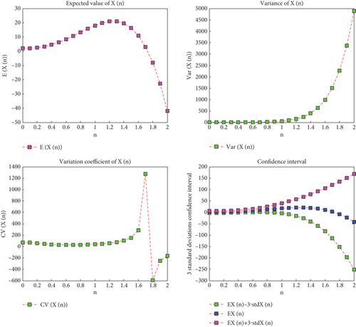
Figure 2 provides the solutions for the expected value, variance, CV, and confidence interval of the n ∈ [0, 2] distribution. The data shows a gradual initial increase followed by a subsequent fall in the expected value, but the variance exhibits a rapid and significant increase, indicating a substantial rise in random effects.

Table 2 provides the expected value, variance, and confidence interval for K = 3 values. As can be observed, the outcomes for values of n ∈ [0, 1] are obtained in a manner akin to that of the case with geometrical and Poisson parameters.

Example 3. Consider the following linear difference equation with variable coefficients:

(23)

Table 2. Table displaying the statistical measures of expected value, variance, coefficient of variation, and 99% confidence interval.

n	E[X(n)]	Var[X(n)]	CV[X(n)]	E[X(n)] − 3Std[X(n)]	E[X(n)] + 3Std[X(n)]
0	2	2	70.710678	−2.242640	6.242640
0.1	1.999737	2.024747	71.156150	−2.269071	6.268545
0.2	2.398769	2.119308	60.688813	−1.968584	6.766122
0.3	3.243344	2.351539	47.280599	−1.357073	7.843763
0.4	4.544127	2.860287	37.218112	0.529587	9.617842
0.5	6.276193	3.903728	31.480635	0.348836	12.20355
0.6	8.379034	5.946421	29.102738	1.063449	15.69461
0.7	10.75655	9.804476	29.109787	1.362924	20.15018
0.8	13.27707	16.87378	30.938832	0.953758	25.60038
0.9	15.77331	29.47173	34.417538	0.513045	32.05968
1	18.04244	51.32852	39.708558	−3.450738	39.53561

Let us examine the solution behaviour of the equation A ~ B(p, q) with binomially distributed random variables p = 4/5, q = 1/5.

The initial conditions are as follows:

(24)

Using Theorems 5, 7, and 10, the differential transformation method of Equation (15) is obtained as follows:

(25)

where N is a sufficiently large integer. The BCs in Equation (24) can be transformed at x₀ = 0 as follows:

(26)

Taking N = 4, the following system of equations can be obtained from Equation (25) for k = 0, 1, 2.

(27)

From the system of Equation (27), we obtain

(28)

Then, using the inverse transformation rule in Equation (2), we obtain

(29)

where α = x^′(0) = X(1) missing BC. The numerical value of α is obtained from the second part of Equation (26) as α = 86A(1 − 3ⁿ⁺¹). Then Equation (29) becomes

(30)

It can be seen from Equations (28) and (29) that the coefficients of the series vary with N, which is a consequence of the implicit behaviour of the solution technique. With N = 4, comparative numerical results and the exact solution x(n) = 3ⁿA are obtained. Binomial distributions are used. Moment extractor function X ~ B(p, q).

( )

Here is the expected value and its variance:

( )

Let us find the probability characteristics of the solution obtained from Equation (30). Firstly, the expected value

( )

The variance is as follows:

( )

Let A, ~Bi(p = 1/5, q = 4/5) be the parameters. The numerical characteristics of the approximate solutions of the obtained random linear difference equation are obtained by calculating the following:

( )

is obtained and variance,

( )

CV is calculated as 100 × std(X(n))/E(X(n)) by definition. The CV is

( )

is obtained.

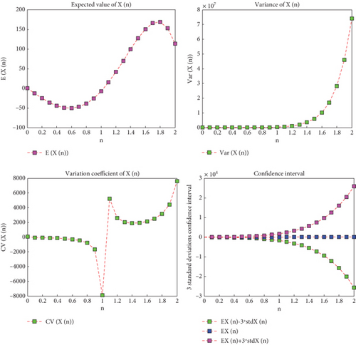
Figure 3 provides the solutions for the anticipated value, variance, CV, and confidence interval of n ∈ [0, 2]. The observed trend shows that the anticipated value initially experiences a tiny fall, followed by an increase, and then another decrease. Meanwhile, the variance remains constant initially but increases significantly after the value of n reaches 1.4, indicating a substantial rise in random effects.

Table 3 provides the expected value, variance, and confidence interval for K = 3 values. As can be observed, the outcomes for values of n ∈ [0, 1] are obtained in a manner akin to that of the case with binomial parameters. In the present study, the approximate analytical series solution was obtained by applying the differential transformation method to ordinary random difference equations. Since DTM is a Taylor series–based method, the accuracy and speed of random DTM provide quite accurate results for the mean, variance, and confidence interval functions of a random difference equation. There are few studies in the literature on approximate analytical solutions of random difference equations. As a result, this method is easy and efficient to apply to linear and nonlinear random difference equations where the randomness in the equation is introduced by analytical m.f.stochastic processes.

Table 3. The variance, coefficient of variation, expected value, and 99% confidence interval are presented in the following table.

n	E[X(n)]	Var[X(n)]	CV[X(n)]	E[X(n)] − 3Std[X(n)]	E[X(n)] + 3Std[X(n)]
0	0.8	0.16	50	0.400000	2
0.1	−12.75742	67.28754	−64.29899	−37.36612	11.851266
0.2	−25.35018	395.5429	−78.45412	−85.01496	34.314606
0.3	−36.15602	1350.502	−101.6405	−146.4035	74.091530
0.4	−44.39071	3719.446	−137.3874	−227.3525	138.57107
0.5	−49.33056	9104.636	−193.4261	−335.5852	236.92408
0.6	−50.33969	20619.57	−285.2524	−481.1252	380.44586
0.7	−46.90238	44092.02	−447.6979	−676.8454	583.04068
0.8	−38.66109	90101.09	−776.4095	−939.1664	861.84425
0.9	−25.46019	177367.9	−1654.153	−1288.912	1237.9921
1	−7.395918	338316.3	−7864.468	−1752.345	1737.5532

6. Conclusion

In this study, the random effects of different distributions on difference equations are investigated by using the differential transformation method. The expected value, variance, CV, and confidence intervals of the solutions of random difference equations are calculated by applying the discrete probability distributions of uniform distribution, Bernoulli distribution, geometric distribution, binomial distribution, and Poisson distribution to the series solutions of three linear random difference equations. In the first examples given, by using the uniform distribution for the expected value, it is seen that the expected value is at the highest level at n = 0 and the value E[X(0)] = 3 is obtained, and for the variance, it is shown that there is a random effect using the Bernoulli distribution, and this random effect is shown in the table. Similarly, in the second example, using the geometric distribution of the expected value, it is seen that the expected value is at the highest level at n = 1 and the value E[X(1)] = 18.04244 is obtained, and the variance is randomised using the Poisson distribution and these effects are tabulated. In Example 3, since there is only one variable; only the binomial distribution is applied, and it is seen that the expected value is at the highest level at n = 2 and the random effect of E[X(1)] = 168.5 is calculated and written in a table. The obtained series solutions are compared with the exact solutions, and the numerical results are shown to be a suitable method for the DTM difference equation solution.

Conflicts of Interest

The authors declare no conflicts of interest

Author Contributions

All authors have contributed equally to the study. The authors have read and agreed to the published version of the manuscript.

Funding

The authors received no specific funding for this work.

Open Research

Data Availability Statement

Data sharing is not applicable to this article.

References

1 Zhou J. K., Differential Transformation and Its Applications for Electrical Circuits, 1986, Huazhong University Press, Wuhan.
Google Scholar
2 Ayaz F., Solutions of the system of differential equations by differential transform method, Applied Mathematics and Computation. (2004) 147, no. 2, 547–567, https://doi.org/10.1016/S0096-3003(02)00794-4, 2-s2.0-0141961581.
10.1016/S0096-3003(02)00794-4
Web of Science® Google Scholar
3 Abbasov A. and Bahadir A. R., The investigation of the transient regimes in the nonlinear systems by the generalized classical method, Mathematical Problems in Engineering. (2005) 2005, no. 5, 519, https://doi.org/10.1155/MPE.2005.503, 2-s2.0-31044448954.
10.1155/MPE.2005.503
Google Scholar
4 Abdel I. H. and Hassan H., Application to differential transformation method for solving systems of differential equations, Applied Mathematical Modelling. (2008) 32, no. 12, 2552–2559, https://doi.org/10.1016/j.apm.2007.09.025, 2-s2.0-50149090462.
10.1016/j.apm.2007.09.025
Google Scholar
5 Merdan M. and Şişman Ş., Investigation of linear difference equations with random effects, Advances in Difference Equations. (2020) 579, 1–19, https://doi.org/10.1186/s13662-020-03018-9.
10.1186/s13662-020-03018-9
Google Scholar
6 AlAhmad S., Mamat M., and AlAhmad R., Finding differential transform using difference equations, IAENG International Journal of Applied Mathematics. (2020) 50.
Google Scholar
7 Merdan M. and Şişman Ş., Analysis of random discrete time logistic model, Sigma Journal of Engineering and Natural Sciences. (2020) 38, 1269–1298.
Google Scholar
8 Şişman Ş. and Merdan M., On the solution of random linear difference equations with Laplace transform method, Mathematical Methods in the Applied Sciences. (2023) 46, no. 17, 18258–18273, https://doi.org/10.1002/mma.9556.
10.1002/mma.9556
Google Scholar
9 Arikoglu A. and Ozkol I., Solution of difference equations by using differential transform method, Applied Mathematics and Computation. (2006) 174, no. 2, 1216–1228, https://doi.org/10.1016/j.amc.2005.06.013, 2-s2.0-33644589650.
10.1016/j.amc.2005.06.013
Web of Science® Google Scholar
10 AlAhmad S., Mamat M., AlAhmad R., Sulaiman I. M., Ghazali P. L., and Mohamed M. A., On new properties of differential transform via difference equations, International Journal of Engineering & Technology. (2018) 7, 321–324.
Google Scholar
11 Yüzbaşı Ş. and Ismailov N., Differential transform method to solve two-dimensional Volterra integral equations with proportional delays, New Trends in Mathematical Sciences. (2017) 5, no. 4, 65–71.
10.20852/ntmsci.2017.215
Google Scholar
12 Yüzbaşı Ş. and Ismailov N., Solving systems of Volterra integral and integrodifferential equations with proportional delays by differential transformation method, Journal of Mathematics. (2014) 2014, 5, 725648, https://doi.org/10.1155/2014/725648, 2-s2.0-84993676175.
10.1155/2014/725648
Google Scholar
13 Keskin Y. and Oturanc G., Reduced differential transform method for partial differential equations, International Journal of Nonlinear Sciences and Numerical Simulation. (2009) 10, no. 6, 741–750.
10.1515/IJNSNS.2009.10.6.741
Web of Science® Google Scholar
14 Abdel-Halim Hassan I. H., Different applications for the differential transformation in the differential equations, Applied Mathematics and Computation. (2002) 129, no. 2-3, 183–201, https://doi.org/10.1016/S0096-3003(01)00037-6, 2-s2.0-0037054950.
10.1016/S0096-3003(01)00037-6
Web of Science® Google Scholar
15 Arikoglu A. and Ozkol I., Solution of fractional differential equations by using differential transform method, Chaos, Solitons & Fractals. (2007) 34, no. 5, 1473–1481, https://doi.org/10.1016/j.chaos.2006.09.004, 2-s2.0-34250215244.
10.1016/j.chaos.2006.09.004
Web of Science® Google Scholar
16 Odibat Z. M., Bertelle C., Aziz-Alaoui M. A., and Duchamp G. H. E., A multi-step differential transform method and application to non-chaotic or chaotic systems, Computers & Mathematics with Applications. (2010) 59, no. 4, 1462–1472, https://doi.org/10.1016/j.camwa.2009.11.005, 2-s2.0-75349091961.
10.1016/j.camwa.2009.11.005
Web of Science® Google Scholar
17 Ertürk V. S. and Momani S., Solving systems of fractional differential equations using differential transform method, Journal of Computational and Applied Mathematics. (2008) 215, no. 1, 142–151, https://doi.org/10.1016/j.cam.2007.03.029, 2-s2.0-39849101342.
10.1016/j.cam.2007.03.029
Web of Science® Google Scholar
18 Feller W., An Introduction to Probability Theory and Its Applications, Volume 1, 1968, 3rd edition, John Wiley & Sons, New York.
Google Scholar

All articles

Analysis of Random Difference Equations Using the Differential Transformation Method

Abstract

1. Introduction

2. Differential Transformation Method

3. Solution Techniques for Difference Equation