Stochastic programming has become increasingly vital in energy applications, especially in the context of the growing need for renewable energy solutions. This paper presents a significant advancement in this field by introducing an efficient and robust algorithm for optimally sizing hybrid renewable energy systems. Utilizing a two-stage stochastic programming approach, the proposed algorithm addresses the challenges posed by the unpredictability of renewable energy sources. The proposed solution leverages the three-block alternating direction method of multipliers (ADMM), a cutting-edge technique that facilitates parallel computation and enhances computational efficiency. The distinctiveness of this method lies in its ability to solve complex stochastic optimization problems without compromising the mathematical integrity of the model. This is achieved by applying first-order optimality conditions, ensuring both robustness and efficacy. To demonstrate the practical applicability and superiority of the algorithm, a case study was conducted in a rural area of South Africa. The proposed algorithm was applied to design an optimal hybrid renewable energy system, and its performance was compared against traditional methods such as progressive hedging and Monte Carlo techniques. Results affirm the superiority of the approach, saving approximately 8.16% capital cost when compared to progressive hedging. In addition, the proposed algorithm outperforms the Monte Carlo method both in terms of CPU time and the number of cost function evaluations.

1. Introduction

Two types of methods are used in generating electricity: conventional and renewable. The first type, particularly oil-based generation plants, is crucial for its ability to guarantee stable energy production and thus cannot be entirely replaced. Conventional methods, such as oil, gas, and coal, are popular for their deterministic nature. The second type consists of renewable methods.

Recent literature emphasizes the potential of renewable energy in reducing greenhouse gas emissions and offering cost-effective solutions [1, 2]. These studies explore technical advancements and the economic viability of renewable systems, underlining the importance of innovative designs and optimization models [3, 4].

Adapting renewable methods, which depend on natural resources obtained from the environment, such as the sun, wind, hydro, hydrogen, and geothermal, is essential to decrease dependency on nonrenewable sources. This adaptation is vital due to the essential shortcomings of conventional methods, like their dependence on depleting fossil fuels that are not evenly distributed worldwide. Moreover, reducing toxic gases like carbon dioxide and carbon monoxide, known as greenhouse gas emissions, is important.

From an economic perspective, the initial construction costs for conventional generators are reasonably suitable. However, the running costs are extremely high compared to renewable ones. This is due to the continuous demand for fuel to keep the generator running.

Under these circumstances, scientists and engineers have worked hard to find alternative methods to generate electricity effectively and reliably to meet the demand and keep the environment unharmed. The innovative approaches should minimize greenhouse gas emissions to an acceptable level and accommodate future population growth and related human activities. Renewable sources are considered a well-suited solution for power generation since they use free natural resources that are not depletable and produce clean power. Although the installation costs of renewable systems are high, the operating costs are much lower than those of conventional methods in long-term projects. Weather conditions and seasonal cycles are the main factors affecting electricity production by renewable sources.

Recent studies have highlighted challenges of reliability in renewable systems due to weather fluctuations and proposed various optimization methods to address these issues, including the use of Loss of Power Supply Probability (LPSP) for reliability assessment [5–7]. Additionally, metaheuristic algorithms like Genetic Algorithm (GA) and Particle Swarm Optimization have been investigated for their effectiveness in optimizing hybrid systems [8, 9]. In the evolving landscape of hybrid renewable energy systems (HRES), the last decade has seen significant advancements in sizing methods, primarily through mathematical modeling and optimization techniques. Optimization methods are crucial for determining efficient and cost-effective combinations of renewable energy resources, ensuring a certain reliability level. The use of classical [10], heuristic, and metaheuristic optimization methods, such as Pattern Search, PSO, and Genetic Algorithms, has become prevalent [11, 12]. Despite these advancements, these methods face challenges in constraint handling and dimensionality [13, 14], underscoring the need for continuous research. Moreover, while our model exhibits improvements in computational efficiency and solution convergence over traditional methods, including Monte Carlo and progressive hedging algorithms, through parallel computation, it is noted that its efficiency may decrease as the number of scenarios increases. However, it still maintains a comparative advantage due to its parallel computation capabilities.

Using a single source of renewable energy may affect system reliability. Hybridizing two or more sources, possibly with backup sources like a conventional generator and batteries, will enhance system reliability.

The focus of this study is primarily on exploring the optimal combination and sizing of solar, wind, and hydrogen-based renewable energy systems. While other renewable sources like bioenergy, hydro, and tidal energy are crucial in the broader context, the focus here is on these selected sources due to their increasing relevance and potential in the current renewable energy landscape.

In recent years, determining the optimal size of hybrid renewable energy systems has become increasingly popular. While notable studies have addressed this challenge, existing methodologies have limitations. A proposed approach by Dong et al. [15] involved using photovoltaic (PV), wind power, battery, and hydrogen subsystems as backup suppliers to design an optimal system with lower annual costs and higher reliability. However, their use of Ant Colony Optimization did not guarantee optimal solutions. Other studies [16] have utilized stochastic programming and Monte Carlo techniques, which can be time-consuming and computationally intensive.

Mathematical optimization techniques based on decomposition, such as Benders’ decomposition and progressive hedging (PH), have been suggested [17] for dealing with large problem sizes. Such techniques generally require multiple solutions of subproblems and may also depend on the optimization problem at hand. Many heuristics and metaheuristics have also been suggested in the literature [18–21]. However, solutions obtained by such heuristics cannot be verified mathematically. Moreover, these methods cannot be applied to problems with a large number of constraints. Hence, the numerical intractability of the problem with many variables and constraints remains a drawback.

This paper proposes an efficient algorithm for the optimal sizing of hybrid renewable energy systems using a two-stage stochastic programming approach. The approach maintains the integrity of the mathematical model for numerical tractability and employs first-order optimality conditions, ensuring robustness and efficacy in solving complex stochastic optimization problems. Utilizing the state-of-the-art three-block alternating direction method of multipliers (ADMM), the algorithm inherently supports parallel computation, facilitating the efficient resolution of the model. By leveraging specific power demand data for the target region, this method provides a robust framework for determining the optimal configuration of renewable energy systems. Notably, the proposed mathematical procedure and optimization technique demonstrate clear advantages over traditional Monte Carlo and progressive hedging algorithms, including enhanced computational efficiency and guaranteed convergence. These benefits are instrumental for the model’s wide applicability in various settings, addressing the critical need for efficient and effective renewable energy system optimization.

The rest of the paper is organized as follows. Section 2 overviews the features of renewable power used in the study. Section 3 presents the mathematical formulation of two-stage stochastic programming (SP) using ADMM. Section 4 introduces the optimization of the renewable energy system. Section 5 applies the optimization of two-stage SP to build a hybrid renewable energy system in a South African village as a case study and compares it with the results obtained using PH. Section 6 establishes the efficiency of the three-block ADMM with a two-stage SP based on Monte Carlo using another case study from the literature. Section 7 concludes the paper.

2. Hybrid Power System

Renewable energy depends solely on weather conditions, which may affect system reliability. For any energy system that uses renewable energy sources, hybridizing two or more power generation methods with backup sources, like a conventional generator and batteries, will enhance system reliability. This section provides a preview of three types of renewable plants for generating electric power.

2.1. Solar System

Constructing a solar farm requires choosing a suitable location that maintains a good potential for solar intensity. Performing a feasibility study for the location site requires at least one year of solar data to analyze the solar reliability in that location.

The power produced by each PV cell at a specified time t is given by

(1)

where p_pv,rated is the generated power by the PV cell at the standard temperature conditions at time t (1 kW/m² solar irradiance, 25°C air temperature, and 1.5 air mass [22]), G(t) is the perpendicular solar insolation at the PV cell surface at time t, G_STC is the solar insolation at the standard temperature condition, and η_pv is the efficiency factor of the PV cell which is determined by many factors like the aging of the panel, deviation of the temperature from 25°C, and other factors. The total power produced by the PV system at time t is given by

(2)

where N_pv is the number of cells.

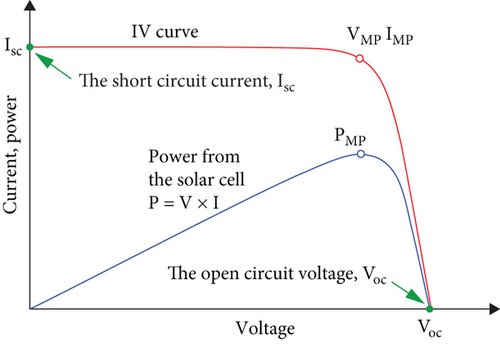
We present the IV (current-voltage) curve of a PV panel on Figure 1, a crucial characteristic for understanding its performance. The curve is plotted with voltage on the x-axis and both current and power on the y-axis. Key points on this curve include the short-circuit current (I_SC), where the curve meets the current axis indicating the maximum current with no voltage, and the open-circuit voltage (V_OC), where the curve intersects the voltage axis showing the maximum voltage with no current flow. The maximum power point (P_MP) is another critical aspect, represented by V_mp (voltage at maximum power) and I_MP (current at maximum power), indicating where the product of voltage and current (P = V × I) is at its peak. This point is where the PV panel operates at its optimum efficiency. The curve visually demonstrates how the PV panel’s power output varies with changes in voltage and current, providing essential insights for optimizing solar energy systems.

Details are in the caption following the image — **Figure 1**
Open in figure viewer PowerPoint

Current-voltage (IV) curve of a solar cell [23].

2.2. Wind Energy

The rapid growth of technologies and research helps the development of wind turbine design, which is providing its worth as the percentage of power generated by the wind grows. Wind power is heavily influenced by wind speed and hub height, where hub height is the height of a wind turbine from the ground.

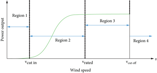
Wind turbine power is closely dependent on wind speed. At a minimal cut-in speed, the turbine begins to generate power. When the wind speed surpasses the maximum cut-out speed, making the turbine potentially dangerous, a braking mechanism, which can be either aerodynamic or mechanical, is employed to safely halt the turbine. The maximum power generated by a wind turbine, known as rated power, is attained at the rated wind speed [3].

The general shape of the power curve of a wind turbine appears in Figure 2. The power curve depicts the connection between wind turbine power output and wind speed. At a time t, the amount of power produced by a wind turbine is given by [24]

(3)

where P_rated is the rated (maximum) power of the turbine in kilowatt (kW), v_cutin is the cut-in speed (m/s), v_cutout is the cut-out speed (m/s), and v is the wind speed (m/s) [25].

2.3. Hydrogen Energy

In recent years, there has been a surge in interest in hydrogen and fuel cell technologies, which are seen as clean, dependable renewable energy sources. The fuel cells that use hydrogen as fuel produce no harmful emissions. These technologies are considered an effective solution to greenhouse gas-free 21st century.

Hydrogen is not an energy source, but it is an energy carrier. The hydrogen H₂ is the most abundant element in the universe [26, 27] since the sun consists of 70% of hydrogen and 28% of helium. Although hydrogen is an abundant amount in the universe, it is less likely to be found alone in nature. Usually, it creates a compound with other chemical elements due to its chemical bonds. Since hydrogen can not be alone, one way of producing hydrogen—without chemical waste and environmental damage—is to use water as a source of hydrogen distillation. Water splitting is the technique of obtaining hydrogen from water. This method employs either electricity (electrolysis) or heat (thermolysis). In the system that we intend to develop in this research, we plan to use the excess electricity of renewable energy to produce hydrogen by the electrolysis method.

When the generated power exceeds the load demand, the remaining one is transferred into hydrogen. The following equation describes the power transfer from the electrolyzer to the hydrogen tank [5]:

(4)

where P_el−tank is the power transferred from the electrolyzer to the hydrogen tank, P_g−el is the generator’s surplus power provided to the electrolyzer, and η_el is the electrolyzer efficiency. The energy of hydrogen contained in tanks at time t is calculated as follows:

(5)

where E_tank(t) stands for the amount of energy stored in the tank at time t, P_tank−fc(t) is the amount of power generated by fuel cells using the hydrogen from the tank at time t, and η_tank is the storage efficiency.

3. Two-Stage Stochastic Programming Using ADMM

3.1. Two-Stage Stochastic Programming

Define the two-stage stochastic programming (SP) as

(6)

(7)

where

, and

are constants and E is the expected value over the the random variable ξ that follows a known distribution [28]. The term

outlines the second-stage optimum value and is defined as [29]

(8)

where

, and

encode the random variable data [30].

The value of the first-stage variable, x, needs to be determined before any future revealing of the random variable ξ; y is known as the second-stage decision variable, which corresponds to the decisions after the realizations of the random variable revealed; y(ξ) is also known as recourse decision variable since it compensates any bad decisions that may occur at the first stage.

When the random variable ξ has finitely many realizations, or scenarios S = {ξ₁, ξ₂.⋯, ξ_s}, with corresponding probabilities {p₁, p₂, ⋯, p_s}, problem (6) can be reformulated as a large linear programming (LP) problem [31] in the form

(9)

(10)

(11)

(12)

where ξ = ξ_i is the i-th scenario.

The proposed algorithm solves the two-stage problem when the recourse matrix, W, is random or constant. Problem (9) can be equivalently restated as

(13)

(14)

(15)

(16)

(17)

where

(18)

is a convex function since it is defined on a convex set [32].

The two indicator functions in (13) for the pairs compensate for the nonnegativity condition of the variables x and y_i in the constraints (15) and (16), respectively. The new formulation in Equations (13)–(17) is considered as a three-block ADMM model. The first-stage decision variable x is presented in the first block, while the second-stage decision variable y_i in the second block and the third one for the pair [29].

3.2. Three-Block ADMM

The classic 2-block ADMM, its numerical implementation, and convergence properties have been established in the literature [33–35]. Sun et al. [36] have applied an extension called 3-block semiproximal ADMM to a class of convex conic programming with four types of constraints. The 3-block ADMM has now been implemented in stochastic programming, which addresses a wide range of problems than the classical one. To the best of our knowledge, this is the first application that uses 3-block ADMM to solve energy-related two-stage stochastic programming problems.

Define the three-block minimization problem as follows:

(19)

(20)

where

are proper lower semicontinuous functions,

is a linear function, b ∈ ℝ^m, and A₁, A₂, and A₃ are in appropriate dimensions [37]. The augmented Lagrangian for problem (19) is defined as

(21)

Regularized terms are added to the solution procedure of problem (19). These terms enhance convergence by reducing oscillation between progressive iterates [38]. The following iterative procedure incorporates these regularized terms:

(22)

(23)

(24)

(25)

where λ is a penalty parameter linked with the regularized terms. The augmented regularized term added to each subproblem in (22) eliminates the need for a convex objective function [29, 37].

Boyd et al. [33] state the necessary and sufficient optimality conditions for problem (19) as follows:

(26)

(27)

(28)

(29)

where Equation (26) is the primal feasibility and Equations (27)–(29) are dual feasibilities. Here, ∂f denotes the subdifferential set of f (see [37]).

Provided that

minimizes

, we have

(30)

which means that

and μ^k+1 satisfy the duality condition in Equation (29).

In the case of

, we have

(31)

where

(32)

is the residual for the dual feasibility.

By repeating the same steps, we find the residual associated with

(33)

At iteration k + 1, using the last equation of (22), we define

(34)

as primal residual and

as dual residuals [33]. We have proved the convergence of the three-block ADMM and showed that all residuals converge to zero as k⟶∞ in [10].

3.3. Solving Two-Stage SP Using Three-Block ADMM

The deterministic version of the two-stage SP (13)–(17) is considered, along with the notations used therein. The variables x₁, x₂, and x₃ of Equation (19) are redefined as

, and x₃≔x to solve the two-stage SP as 3-block ADMM. Correspondingly, the functions will be defined as follows:

(35)

In what follows, the detailed steps to find the solution to problem (13)–(17) are derived, followed by a presentation of a step-by-step algorithm for the solution. Consider the following augmented Lagrangian function:

(36)

where

, and

, i = 1, 2, ⋯, s. The vector of multipliers is defined as

(37)

Solving

for x^k+1 yields

(38)

Similarly,

for

yields

(39)

which allows parallel computing, enabling the concurrent solution of all equations associated with the scenarios.

And by differentiating

and

with respect to

, respectively, yields

(40)

(41)

The updates for the dual variables will be expressed as

(42)

(43)

(44)

(45)

Updating of γ_i, δ_i in (42) and in (40) together with (33) and (34) is also performed in parallel.

Algorithm 1 presents the steps of ADMM for solving two-stage SP in Equations (13)–(17). An important parameter of Algorithm 1 is the penalization parameter ρ. The convergence of the ADMM algorithm is very sensitive to ρ; poor selection may lead to slow or nonconvergence in practical problems [39]. A variant of ADMM, residual balancing, where the penalty parameter ρ_k changes at each iteration k is proposed in [40]. The intuition behind the method is based on making the primal and dual residual norms have similar magnitudes. By doing so, the primal and dual residuals will have small values at the stage of convergence. This approach makes the performance less dependent on the initial choice of ρ. The superlinear convergence with ρ_k⟶∞ has been achieved in [41]. An iteration-dependent adaptive ρ_k, as suggested in [40], is implemented. In Algorithm 1, the preconditioning step initializes penalty parameter ρ, the maximum number of iterations k_max, and the convergence tolerance ε. The initialization in line 1 provides an initial first-stage solution for the primary iterations k ≥ 1. The initial penalty parameter will be adaptively updated in [40] to maintain the gap difference between the primal and dual residuals (see Equation (46)). Algorithm 1 runs on deterministic initializations, in which the first phase procedure of linear programming is applied to bring the starting point to a feasible region. Since Algorithm 1 decomposes the problem by scenarios, lines 5, 8, 12, 13, 15, and 18 are implemented in parallel. Line 5 provides a scenario-wise solution to the second-stage variable in parallel. The second-stage solution needs to be assembled in one variable to find the first-stage solution, which is given in line 9. Lines 10-13 give the updates for the dual variables using (42). The primal and dual residuals of Algorithm 1 are given in lines 14-19. Algorithm 1 terminates in two ways: the convergence case, where all the residuals are less than the threshold ε, line 20, or the nonconvergence case, line 21, where the algorithm hits the maximum number of iterations without meeting the convergence requirements. In the nonconvergence case, the algorithm is enforced to stop by the maximum iteration [29].

In the initialization step, we have defined the penalty parameter ρ as [40]

(46)

where ν > 1 and μ > 1. We choose ν = 2 and μ = 4. The values ε = 10⁻³ and k_max = 5 × 10⁴ were used, respectively, in steps 20 and 21 of Algorithm 1. The primal and dual residuals are given in line 19 of Algorithm 1, where r is the primal residual and s¹ and s² are the dual residuals.

Algorithm 1: Solving two-stage SP using ADMM.

Precondition: ρ > 0, λ, k_max > 0, ε > 0. All the initialization to the variables are obtained by first phase Linear Programming (LP) step, while are random variables following the standard normal distribution.
1:
2: k⟵1
3: while True do
4: for i⟵1 to sdo
5:
6: end for
7:
8:
9:
10: α^k+1⟵α^k + ρ(Ax^k+1 − b)
11:
12:
13:
14: r₀⟵Ax^k+1 − b
15:
16:
17:
18:
19:
20: If ‖r‖≤ ε, ‖s¹‖ ≤ ε, and ‖s²‖ ≤ ε stop; otherwise k⟵k + 1
21: If k equals k_max, stop; the algorithm does not converge.
22: end while

4. Optimization of Hybrid Renewable Energy

The optimization problem for a hybrid renewable system will be formulated by constructing an objective function along with the constraints throughout the remainder of this section.

4.1. Reliability of the System

The uncertainty of weather conditions leads to fluctuating energy production, which has an impact on the system’s reliability. The LPSP is employed as an index for reliability estimation. In the constraints, a specific level of reliability is ensured to meet the system demand by a designated probability percentage of LPSP. The system reliability for the time interval T, as given in [42], is described in terms of LPSP and expressed as

(47)

where LPS(t) is the loss of power supply at time t and given by

(48)

where P_l(t) and P_g(t) are the required load and the generated power, respectively, at time t. The system will be more reliable when it has a small LPSP, α⟶0, and less reliable when it is large, α⟶1. We can write Equation (47) as

(49)

4.2. The Mathematical Model

We assume that the projected demand for electricity follows a known probability distribution. We consider m blocks of demand for various quantities of power throughout the year. The formulation of the objective function for n different renewable energy plants at m demand blocks of generation in t years is given by

(50)

(51)

(52)

(53)

(54)

where c_k is the investment cost per kilowatt (kW) of the power plant k, x_k is the capacity in kW to build for the power plant k, b is the total allocated budget, y_kjlω is the amount of electricity capacity used to produce electricity by power plant k for demand block j in year l under scenario ω measured in kW, d_jlω is the load demand in year l at block j under scenario ω in kW, α is the factor of LPSP, q_kω is the operating cost of unit k under scenario ω in $/kWh, and τ_j is the duration of the demand at block j in hours.

The objective function in Equation (50) determines the cost for kW capacity to be built for each plant together with the operating cost. The constraint in Equation (51) represents the reliability condition as the power generated by the hybrid system should meet a minimum level of reliability given by α. Equation (52) ensures that the electricity generated by unit k does not exceed the total capacity of that unit. Equation (53) guarantees that the investment cost does not surpass the available budget.

To monitor the times when the system uses the power supplied by each plant or a combination of them, a number of modes can be used to track the system’s behavior. An example of this is shown in Section 5.2.

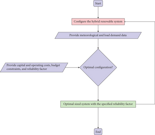
The problem, therefore, is to design an optimal sizing system of hybrid renewable energy that ensures system reliability using SP based on three-block ADMM and the concept of LPSP. Such ecofriendly systems seek to minimize the effect of greenhouse gas emissions by using entire renewable sources. Figure 3 represents a possible flowchart of the optimal sizing process for the hybrid renewable energy system (HRES) components.

5. Case Study: Ga-Nkoana

In this study, an analysis is conducted to construct a hybrid renewable energy system in the village of Ga-Nkoana to meet both current and future electrical power demands. Ga-Nkoana is a suburb located in Limpopo province, South Africa, with coordinates at a latitude of -24.416673° and a longitude of 29.783335°. According to the 2011 SA census, Ga-Nkoana has a population of 443 households. Assuming an annual household growth rate of 3% and using the logistic growth equation with a carrying capacity of K = 10,000 [43], the estimated number of households by the year 2023 will be approximately 623. The renewable system is intended to be constructed once and used for the entire project duration of 20 years. For this study, four renewable resources are considered: solar power (x₁), wind power (x₁), hydrogen power (x₃), and backup batteries (x₄). The initial budget allocated for this construction is set at $120,000. The primary objective is to determine the optimal combination of these renewable plants that minimizes the sum of the capital cost and the expected operating cost over the course of 20 years while ensuring a specified reliability percentage using LPSP. The operating cost is assumed to be stochastic due to the uncertainty in weather conditions and fluctuating load demand.

The hourly load day for Ga-Nkoana is obtained from the Domestic Electrical Load Metering Data (DELM) between 1994 and 2014 available in DataFirst’s secure center [44]. The climatic data for the village is obtained from the Prediction of Worldwide Energy Resources (POWER) [45] project from 2013 to 2020, run by NASA. The data consist of temperature at 2-meter height, wind speeds at 10-meter height, and solar irradiance.

The load data for 632 residential households in Ga-Nkoana has been aggregated to represent the monthly load profile for the entire village. Table 1 displays the average monthly load profile along with data on solar irradiance, wind speed, and temperature. The average annual load is 6.837 kW, which is relatively low compared to urban areas. Additionally, it is observed that the average load remains fairly consistent throughout the months, with a slight increase in January. The yearly growth rate for the demand load is assumed to align with the population growth rate of 3%, accounting for annual increases due to population growth. The table also provides information on the average temperature, a significant factor influencing power generation by PV cells. Notably, the highest temperatures and solar irradiance occur during the summer months of December and January, while the lowest values are recorded in June and July, corresponding to the winter season. Consequently, peak solar power output is expected during months with higher temperatures and solar irradiance. In contrast, the highest wind speed is observed in October, while the lowest occurs in May. This indicates that wind turbines are most productive during months with elevated wind speeds.

Table 1. Monthly average load and climatic data for Ga-Nkoana.

	Load (kW)	Solar irradiance (W/m²)	Wind speed (m/s)	Temperature (C°)
January	8.60	377.36	3.79	23.03
February	6.42	376.77	3.57	22.67
March	6.55	365.21	3.18	21.55
April	6.91	343.62	3.11	19.20
May	6.45	303.55	2.95	16.51
June	6.68	282.99	3.39	13.67
July	7.01	284.19	3.60	13.61
August	6.87	300.19	3.91	16.66
September	6.80	327.52	4.39	19.99
October	6.67	351.60	4.70	21.40
November	6.15	367.99	4.34	22.67
December	6.94	380.23	3.81	23.50

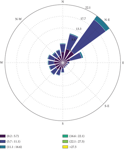
The wind rose in Figure 4 reveals a predominant wind direction, marked by the longer and denser segments, which is crucial for positioning wind turbines in renewable energy projects. The intensity and frequency of winds from these dominant directions, indicated by the extent and color saturation of the segments, suggest consistent wind patterns that are ideal for wind power generation. Lesser segments in other directions indicate variability, but the primary focus for turbine alignment would be towards the most frequent wind directions. This graph is a valuable tool in site selection for wind farms, ensuring that turbines are optimally placed to maximize energy capture from prevailing winds.

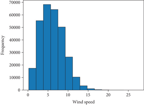
The histogram of Ga-Nkoana’s wind speeds in Figure 5 shows the prevalence and variability of wind in the village. Peaks indicate expected wind speeds, essential for assessing wind energy potential. A concentration at higher speeds suggests favorable conditions for wind power generation. The range of speeds informs turbine selection and expected efficiency, making this data crucial for planning and optimizing wind energy projects in Ga-Nkoana.

The prices of power plants are determined according to their electric capacity, measured in kilowatts (kW). Table 2 shows the capital cost per kW of capacity for each power plant.

Table 2. Capital cost per kW capacity [48–51].

Plant	Cost per kW in $ (c_k)
Solar x₁	3000
Wind turbine x₂	1300
Fuel cell and electrolyzer x₃	1700
Batteries x₄	1500

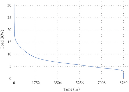
Demands for electric power are described using the load duration curve, which illustrates the relationship between generation capacity requirements and capacity utilization [46]. The load duration curve is ordered in descending order by magnitude. The electric load for Ga-Nkoana using the continuous load duration curve is shown in Figure 6, which displays the load duration curve for 2013 for a total of 8760 hours. For example, in Figure 6, the load was approximately above 5 kW for 5256 h in 2013 and above 9 kW for 1752 h. We obtained the quantized demand set in Table 3 from the continuous curve using the midriser and midtread uniform quantizer [47].

Table 3. Expected power demand data for Ga-Nkoana.

Demand block	Demand (kW) (d_jl)	Duration (hours) (τ_j)
1	23.1380	29
2	18.0440	121
3	12.9510	935
4	7.8570	3134
5	2.7640	4541

5.1. Problem Formulation

A hybrid renewable energy system has been created, utilizing a two-stage SP optimization technique to reduce total investment and operational costs over a certain period. The first-stage variables determine the necessary capacity in kW for each plant, defined by the vector x ∈ R⁴. The sequence of energy sources is as follows: (1) solar, (2) wind, (3) hydrogen, and (4) batteries. The subscript notation x₁, x₂, x₃, x₄ corresponds to each type, respectively. Investment costs are represented by the vector c ∈ R⁴, as detailed in Table 2.

The second-stage variable y corresponds to the decision after the realization of the random event, which represents the capacity used to produce electricity at each power plant for each demand block in each year. The expected power demands over scenarios with the duration of five blocks during the first year are shown in Table 3.

The second-stage decisions depend on stochastic problem data. Each possible value of the stochastic data is called a scenario indexed by ω. For this problem, there are five possibilities of operating costs for PV (see Table 4) and five possible operating costs for wind turbines (see Table 5), for a total of ω = 5 × 5 = 25 scenarios. The reason is that the probabilities of the operating costs are independent.

Table 4. Probability distribution of PV operating costs [48].

Scenario	Cost ($/kWh)	Probability
1	0.0583	10%
2	0.0592	20%
3	0.0603	40%
4	0.0614	20%
5	0.0615	10%

Table 5. Probability distribution of wind turbine operating costs [50].

Scenario	Cost ($/kWh)	Probability
1	0.0141	10%
2	0.0148	20%
3	0.0149	40%
4	0.0153	20%
5	0.0154	10%

The operating costs, q_kω, k = 1, ⋯, 4, and ω = 1, ⋯, 25, for different electricity sources are specified in $/kWh (see Tables 4–6). A growth rate of 3% was applied to estimate the operating costs for subsequent years. The duration in hours of each demand block, τ_j, j = 1, ⋯, 5, is presented in the third column in Table 3. The randsample function in MATLAB was utilized to generate 25 scenarios representing the operating costs for both PV and wind turbine systems, using the probability distribution in Tables 4 and 5. This function facilitated the generation of random data by defining three essential parameters: values, sample size, and probabilities. In this context, the values are the operating costs q_kω, ∀k. The sample size, set at ω = 25, was specified as the second argument to produce the required number of random data points. It should be noted that the operating cost for fuel cell and electrolyzer and batteries will remain constant across all 25 scenarios.

Table 6. Operation cost of power generation.

Plant	Cost $/kWh (q_k)
Solar ^∗	0.060
Wind turbine ^∗	0.015
Fuel cell and electrolyzer	0.025
Backup batteries	0.150

^∗Solar plant and wind turbine operating costs are expected values.

We can write the full optimization formulation as

(55)

(56)

(57)

(58)

where d_jlω is the demand load in block j and year l under scenario ω. Equation (55) was transformed into a linear programming (LP) problem, as formulated in Equation (9), by incorporating the necessary slack and artificial variables. Following this conversion, the budget constraint is represented by Ax = b. Meanwhile, the demand and capacity constraints embody the second-stage constraint Tⁱx + Wⁱy_i = hⁱ, i = 1, 2, ⋯, s.

The size of these problems is enormous, and the standard linear programming (LP) solvers might face difficulties in solving them. There are four first-stage variables and 4 × 5 × 20 × 25 second-stage variables in this problem, for a total of 10,004 variables. There is also one budget constraint, 4 × 5 × 20 × 25 capacity constraints, and 5 × 20 × 25 demand constraints, totaling 12,501 constraints. Such a problem size presents some difficulties to many modern LP solvers. Increasing the number of scenarios will lead to an explosion in the problem size, making the use of the LP solver unrealistic.

5.2. Numerical Experiments and Comparison

This section discusses the numerical experiment of Algorithm 1 implemented to solve the two-stage SP of the hybrid renewable energy system presented above. Results obtained have been compared to progressive hedging (PH). Both algorithms were provided with identical input data, set with a tolerance level of 10^-5, and a predefined maximum iteration limit of 5000. The computer specification that runs the experiments has CPU Intel® Core™ i7-7700 CPU at 3.60 GHz × 8 and 15.5 GB of RAM using MATLAB 2020b. The CPU times for all problems are given. The graphs of the residuals are provided in the log/log scale.

Algorithm 1 and PH were executed using load data for Ga-Nkoana at a Loss of Power Supply Probability (LPSP) of 0.01. Through these computations, the optimal configuration for the hybrid renewable energy system was determined using ADMM and PH, as illustrated in Table 7.

Table 7. Optimal power plant that supply the load of Ga-Nkoana using ADMM and PH.

Plant	Optimal decision using ADMM	Optimal decision using PH
Solar PV	19.31 kW	21.25 kW
Wind turbine	10.83 kW	8.72 kW
Fuel cell	8.84 kW	11.53 kW
Batteries	9.30 kWh	10.22 kWh
Capital cost ($)	101020	110 000
Operating cost ($)	16679	15921
Total cost ($)	117699	125921

Under optimal conditions, these configurations generate a maximum power output of x₁ + x₂ + x₃ = 38.98 kW using ADMM and x₁ + x₂ + x₃ = 41.50 kW using PH. Assuming that the battery can be charged or discharged at a constant rate per hour, the energy storage capacity of the system is 9.30 kWh using ADMM and 10.22 kWh using PH. The associated capital cost for the ADMM configuration amounts to $101,020, while for PH, the total is $110,000. ADMM demonstrates its superiority by offering a substantial cost advantage, saving approximately 8.16% in capital costs compared to PH.

From Figure 7, all the primal-dual residuals of ADMM Algorithm 1 are converged at 76 iterations on the hybrid renewable energy problem. Figure 8 shows the convergence behavior of the objective function to the optimal value. ADMM is notably faster, converging approximately 5.18 times quicker than PH.

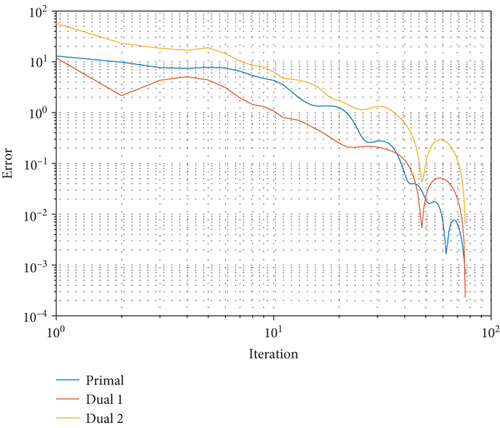
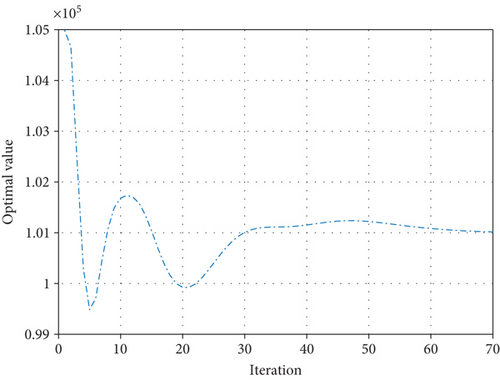
Figure 9 shows the relationship between LPSP and the system cost. As depicted in the figure, a system with small LPSP values and higher system reliability is costlier because it requires building more units of renewable sources to avoid any power outage. Decreasing the tightness of reliability results in a high reduction in the cost of the system, which is good from an economic perspective, but it might have some power outages from time to time.

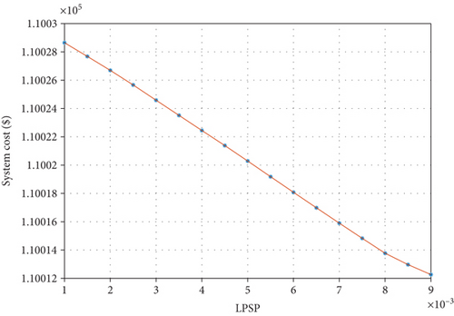
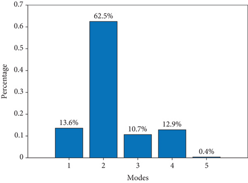
Figure 10 presents a bar plot depicting the five of the hybrid system at a Loss of Power Supply Probability (LPSP) of 0.01. This figure illustrates changes within the system across different modes, based on the optimal solution. It is evident from the figure that wind power alone cannot meet the load demand, as seen in mode 1, where it contributes independently to 13.6% of the system. In mode 2, the hybridization of wind and solar power enhances the system’s robustness, meeting the demand 62.5% of the time. The combination of batteries with wind and solar power, accounting for 10.7% of usage, addresses potential shortages due to peak load demands or weather uncertainties. Mode 4 shows hydrogen power supplying the system 12.9% of the time. It is noted that the system experienced a power outage in 0.4% of instances, as in mode 5, due to setting the LPSP at 1% to achieve 99% reliability.

The reliability of an energy system is strongly related to the system’s energy storage capacity. In finding the optimal sizing of an energy system, it is possible to assign a higher weight to the reliability factor. When doing so, the optimization algorithm prioritizes the fulfillment of having a more reliable system. As a result, the algorithm will naturally adjust the sizing of the energy storage and renewable energy production components, ensuring that they are adequately scaled to meet reliability requirements. This approach guarantees that the energy system can effectively handle variations in renewable energy generation and fluctuations in energy demand, ultimately leading to increased overall reliability. Therefore, in the optimization process, giving greater weight to reliability automatically drives the system towards larger storage and renewable production sizes, solidifying the reliability of the energy system.

6. Comparing ADMM with Monte Carlo Method

The performance of ADMM is compared against another case study presented in [16]. In their research, Sakalauskas and Žilinskas [16] explored power plant investment by addressing a two-stage stochastic programming challenge using Monte Carlo methods. Their study spanned 15 years, with a projected cost of $10 billion for constructing four types of power plants: gas turbines, coal, nuclear power, and hydropower. The study utilized five independent and normally distributed demand blocks to represent varying power consumption levels throughout the year. Table 8 details the mean and standard deviation of the forecasted power demands in gigawatts (GWs) based on the duration of these blocks.

Table 8. Power demand during the year.

Demand block	Expected power demand, (GW)	The standard deviation of power demands, (GW)	Block duration (τ_j)
1	26.0	1.3	490
2	21.5	1.1	730
3	17.3	0.9	2190
4	13.9	0.7	3260
5	11.1	0.6	2090

The price of each power plant is determined based on its electricity production capacity in gigawatts. [16] displayed the investment costs for each plant (see Table 9). They stated that the hydropower capacity does not exceed 5.0 GW due to geographical constraints in the area.

Table 9. The investment costs for power plants.

Power plant type	Cost per GW in billion ($)
Gas turbine	1.1
Coal	1.8
Nuclear power	4.5
Hydroelectric	9.5

Table 10 shows the operating costs and the cost of obtaining power from a third party for the first year of each type of power plant in dollars per kilowatt-hour (kWh).

Table 10. Operating cost of power generation.

Power plant type	Cost ($/kWh)
Gas turbine	0.0392
Coal	0.0244
Nuclear	0.0140
Hydroelectric	0.0040
External source	0.1500

They proposed the two-stage SP formulation for the problem as follows:

(59)

Sakalauskas and Žilinskas [16] applied the Monte Carlo method to expected and stochastic data. They found that the cost of the system based on expected data is $17.137 ± 0.053 billion and the one based on stochastic data is $16.508 ± 0.028 billion. Through this experiment, they argued the importance of using uncertain data in the investment planning of power systems, which costs less than the deterministic approach.

Using the data from Sakalauskas and Žilinskas, the same problem was addressed using both 3-block ADMM and Monte Carlo methods. The ADMM method terminated after 121 iterations, taking only 0.019734 seconds of CPU time. In comparison, the Monte Carlo method needed 123 iterations to converge. While the Monte Carlo method achieved convergence in a moderate number of iterations, it involved a considerably large sample size in the objective function. At each iteration, a sample size of 15,887 was necessary for the sampling objective estimator. The large sample size used in the Monte Carlo method suggests a significantly greater CPU time compared to ADMM. Hence, the results demonstrate the efficiency of the ADMM method over the Monte Carlo method in terms of both computational time and sample size requirements.

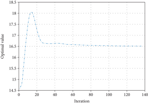
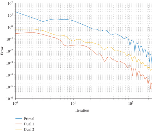
Figures 11 and 12 show the behavior of the optimal objective function and the convergence of ADMM, respectively. Table 11 compares the solutions of Monte Carlo and ADMM using stochastic data. The cost of the system using ADMM is $16.5037 ± 0.023 billion, which is almost identical to their solution. Also, the decisions of the power plants were the same.

Table 11. Optimal power plant sizing based on the stochastic data.

Power plant	Size in GW using Monte Carlo	Size in GW using ADMM
Gas turbine	4.4500	4.4497
Coal	4.3600	4.3593
Nuclear	4.6000	4.6003
Hydroelectric	5.0000	4.9995
Cost (billion $)	16.508 ± 0.028	16.5037 ± 0.023

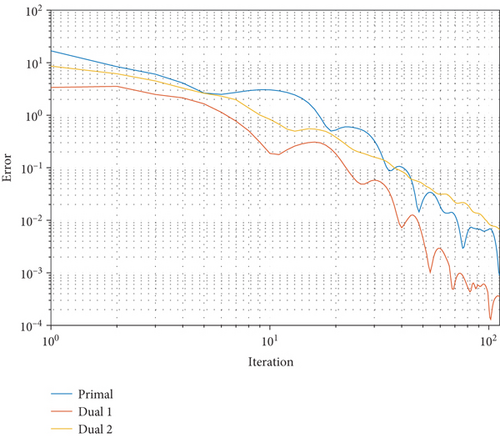
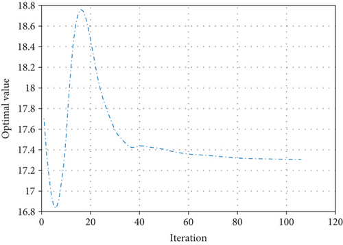
The ADMM method was also applied to the expected data presented by the authors in the second column of Table 8. It was found that ADMM converged after 112 iterations, with a CPU time of 0.035427 seconds. Figure 13 illustrates the convergence behavior of ADMM based on the expected data. The cost calculated using this data is $17.2810 ± 0.0318 billion. Figure 14 displays the convergence of the optimal value using ADMM. The results of both methods, employing the expected data, are provided in Table 12.

Table 12. Optimal power plant sizing based on the expected data.

Power plant	Size in GW using Monte Carlo	Size in GW using ADMM
Gas turbine	1.78	1.7791
Coal	3.23	3.2286
Nuclear	4.07	4.0669
Hydroelectric	5.00	4.9937
Cost (billion $)	$17.137 ± 0.053	17.2810 ± 0.0318

Table 13 presents a comparative summary, highlighting key differences and methodologies between the current study and previous papers. The comparison covers three main categories of optimization techniques: linear programming (LP), nonlinear programming (NLP), and stochastic programming (SP). The symbol ✔ indicates that the method employed the respective methodology, while ✘ signifies its absence. This study is the first to address a sizing problem for hybrid renewable energy using two-stage SP with four types of renewable components, incorporating uncertainty in weather and load demand data.

Table 13. A comparative summary of this study and previous papers.

Ref	Uncertainty	PV	Wind	Hydrogen	Battery	Problem type
[15]	✘	✔	✔	✔	✔	LP
[16]	✘	✘	✘	✘	✘	LP
[52]	✘	✔	✔	✔	✔	—
[24]	✘	✔	✔	✘	✘	NLP
[26]	✘	✘	✔	✔	✔	NLP
This study	✔	✔	✔	✔	✔	SP

7. Conclusion

The two-stage SP with three-block ADMM developed in this study represents a significant advancement in solving stochastic linear programming problems, specifically for optimally sizing hybrid renewable energy systems using stochastic load demand. This method effectively handles the unpredictability of weather and the dynamic load demand that varies throughout the year. The focus on a 20-year period for the renewable system emphasizes commitment to reducing environmental impact, with the entire proposed model being renewable.

The algorithm consistently converges to the optimal point efficiently, as evidenced by reasonable CPU times and the utilization of parallel computing. This approach surpasses the PH method in terms of speed, especially for large-scale problems, and demonstrates its superiority by achieving an 8.16% saving in capital costs compared to PH. The optimal decisions using ADMM for the hybrid power plant in Ga-Nkoana included 19.31 kW for solar PV, 10.83 kW for wind turbine, 8.84 kW for fuel cell, and 9.30 kWh for batteries, with a total capital cost of $101,020. In contrast, the pH method resulted in a slightly different configuration with a higher total cost of $110,000.

Furthermore, addressing the reliability issues in renewable systems, the algorithm uses the LPSP to regulate the reliability percentage, successfully converging to a stable minimizer even with small LPSP values. The validation of this approach, through comparison with Monte Carlo algorithms in existing studies, confirms the correctness and mathematical convergence of the algorithm.

This study is instrumental in implementing hybrid renewable energy systems in regions with load demands similar to Ga-Nkoana, Limpopo, South Africa, leveraging the proposed sizing algorithm’s adaptability for various locations with accessible load demand and weather data. However, a notable shortcoming is the model’s approach of determining the composition of renewable energy systems at the project’s onset, rather than a phased, yearly rollout, which may limit adaptability and elevate operational costs over the 20-year project horizon. Current research is ongoing to address the above issue which we hope to report in near future. Future research could enhance this model by considering the integration of grid-connected power and conventional methods alongside extending its application, offering a comprehensive solution for sustainable energy generation. This direction not only addresses the limitation of initial component determination but also broadens the algorithm’s applicability to more diverse energy systems, contributing to a more adaptable and economically viable framework for renewable energy optimization.

Abbreviations

HRES:: Hybrid renewable energy systems
SP:: Stochastic programming
ADMM:: Alternating direction method of multipliers
LPSP:: Loss of Power Supply Probability
PH:: Progressive hedging
GA:: Genetic Algorithms
kW:: Kilowatt
PV:: Photovoltaic.

Variables

p_pv(t):: The generated power by a PV cell at a specified time t (kW)
p_pv,rated:: The rated power of a PV cell under standard temperature conditions t (kW)
P_pv(t):: The total generated power by the PV system at a specified time t (kW)
G(t):: The perpendicular solar insolation at a PV cell surface at time t (W/m²)
G_STC:: Solar insolation at the standard temperature condition (kW/m²)
η_pv:: Efficiency factor of a PV cell
N_pv:: The number of PV cells
I_SC:: Short-circuit current—the maximum current generated by a PV panel when there is no voltage across it (A)
V_OC:: Open-circuit voltage—the maximum voltage across a PV panel when there is no current flowing through it (V)
P_MP:: Maximum power point—the point on the IV curve where the product of voltage and current is at its peak, indicating optimum efficiency (kW)
V_mp:: Voltage at maximum power—the voltage at the maximum power point (V)
I_MP:: Current at maximum power—the current at the maximum power point (A)
p_wind(t):: The generated power by a wind turbine at time t (kW)
P_rated:: The rated power of a wind turbine (kW)
v(t):: Wind speed at time t (m/s)
v_cut in:: The cut-in speed (m/s)
v_cut out:: The cut-out speed (m/s)
P_el-tank:: Power transferred from the electrolyzer to the hydrogen tank (kW)
P_g−el:: Generator’s surplus power provided to the electrolyzer (kW)
η_el:: Electrolyzer efficiency
E_tank(t):: Energy stored in the tank at time t (kWh)
P_tank-fc(t):: Power generated by fuel cells using the hydrogen from the tank at time t (kW)
η_tank:: Storage efficiency of the tank
c_k:: Investment cost per kilowatt (kW) of the power plant k ($/kW)
x_k:: Capacity in kW to build for the power plant k (kW)
b:: Total allocated budget ($)
y_kjlω:: Amount of electricity capacity used by power plant k for demand block j in year l under scenario ω (kW)
d_jlω:: Load demand in year l at block j under scenario ω (kW)
α:: Factor of LPSP
q_kω:: Operating cost of unit k under scenario ω ($/kWh)
τ_j:: Duration of the demand at block j in hours.

Conflicts of Interest

The authors hereby declare that there are no conflicts of interest regarding the publication of this paper. This includes any financial, personal, or professional affiliations that could be construed as influencing the content or interpretation of the research.

Acknowledgments

Open Access funding was enabled and organized by SANLiC Gold.

Open Research

Data Availability

Data is available on request.

References

1 Yang H., Lu L., and Zhou W., A novel optimization sizing model for hybrid solar-wind power generation system, Solar Energy. (2007) 81, no. 1, 76–84, https://doi.org/10.1016/j.solener.2006.06.010, 2-s2.0-33845993864.
10.1016/j.solener.2006.06.010
Web of Science® Google Scholar
2 Dursun B. and Aykut E., An investigation on wind/PV/fuel cell/battery hybrid renewable energy system for nursing home in Istanbul, Proceedings of the Institution of Mechanical Engineers, Part A: Journal of Power and Energy. (2019) 233, no. 5, 616–625, https://doi.org/10.1177/0957650919840519, 2-s2.0-85063940577.
10.1177/0957650919840519
CAS Web of Science® Google Scholar
3 Bhandari B., Lee K. T., Lee G. Y., Cho Y. M., and Ahn S. H., Optimization of hybrid renewable energy power systems: a review, International Journal of Precision Engineering and Manufacturing-Green Technology. (2015) 2, no. 1, 99–112, https://doi.org/10.1007/s40684-015-0013-z, 2-s2.0-84921342044.
10.1007/s40684-015-0013-z
Web of Science® Google Scholar
4 Baños R., Manzano-Agugliaro F., Montoya F. G., Gil C., Alcayde A., and Gómez J., Optimization methods applied to renewable and sustainable energy: a review, Renewable and Sustainable Energy Reviews. (2011) 15, no. 4, 1753–1766, https://doi.org/10.1016/j.rser.2010.12.008, 2-s2.0-79751534296.
10.1016/j.rser.2010.12.008
Web of Science® Google Scholar
5 Chedid R. and Rahman S., Unit sizing and control of hybrid wind-solar power systems, IEEE Transactions on Energy Conversion. (1997) 12, no. 1, 79–85, https://doi.org/10.1109/60.577284, 2-s2.0-0031104520.
10.1109/60.577284
Web of Science® Google Scholar
6 Yang H., Zhou W., Lu L., and Fang Z., Optimal sizing method for stand-alone hybrid solar–wind system with LPSP technology by using genetic algorithm, Solar Energy. (2008) 82, no. 4, 354–367, https://doi.org/10.1016/j.solener.2007.08.005, 2-s2.0-40949103930.
10.1016/j.solener.2007.08.005
Web of Science® Google Scholar
7 Koutroulis E., Kolokotsa D., Potirakis A., and Kalaitzakis K., Methodology for optimal sizing of stand-alone photovoltaic/wind-generator systems using genetic algorithms, Solar Energy. (2006) 80, no. 9, 1072–1088, https://doi.org/10.1016/j.solener.2005.11.002, 2-s2.0-33746776198.
10.1016/j.solener.2005.11.002
Web of Science® Google Scholar
8 Mohammadi M., Hosseinian S. H., and Gharehpetian G. B., GA-based optimal sizing of microgrid and DG units under pool and hybrid electricity markets, International Journal of Electrical Power & Energy Systems. (2012) 35, no. 1, 83–92, https://doi.org/10.1016/j.ijepes.2011.09.015, 2-s2.0-84855354182.
10.1016/j.ijepes.2011.09.015
Web of Science® Google Scholar
9 Hakimi S. M. and Moghaddas-Tafreshi S. M., Optimal sizing of a stand-alone hybrid power system via particle swarm optimization for Kahnouj area in south-east of Iran, Renewable Energy. (2009) 34, no. 7, 1855–1862, https://doi.org/10.1016/j.renene.2008.11.022, 2-s2.0-61349105917.
10.1016/j.renene.2008.11.022
Web of Science® Google Scholar
10 Mohammed N. and Ali M. M., Stochastic Optimization on Hybrid Renewable Energy Systems. PhD thesis, 2023, School of Computer Science and Applied Mathematics, University of the Witwatersrand, Johannesburg, Gauteng.
Google Scholar
11 AlHajri M. F., El-Naggar K. M., AlRashidi M. R., and Al-Othman A. K., Optimal extraction of solar cell parameters using pattern search, Renewable Energy. (2012) 44, 238–245, https://doi.org/10.1016/j.renene.2012.01.082, 2-s2.0-84858276707.
10.1016/j.renene.2012.01.082
Web of Science® Google Scholar
12 Kumar L. V. S., Kumar G. V. N., and Madichetty S., Pattern search algorithm based automatic online parameter estimation for AGC with effects of wind power, International Journal of Electrical Power & Energy Systems. (2017) 84, 135–142, https://doi.org/10.1016/j.ijepes.2016.05.009, 2-s2.0-84975267309.
10.1016/j.ijepes.2016.05.009
Web of Science® Google Scholar
13 Maleki A., Ameri M., and Keynia F., Scrutiny of multifarious particle swarm optimization for finding the optimal size of a PV/wind/battery hybrid system, Renewable Energy. (2015) 80, 552–563, https://doi.org/10.1016/j.renene.2015.02.045, 2-s2.0-84924597725.
10.1016/j.renene.2015.02.045
Web of Science® Google Scholar
14 Lian J., Zhang Y., Ma C., Yang Y., and Chaima E., A review on recent sizing methodologies of hybrid renewable energy systems, Energy Conversion and Management. (2019) 199, https://doi.org/10.1016/j.enconman.2019.112027, 2-s2.0-85072228410.
10.1016/j.enconman.2019.112027
Web of Science® Google Scholar
15 Dong W., Li Y., and Xiang J., Optimal sizing of a stand-alone hybrid power system based on battery/hydrogen with an improved ant colony optimization, Energies. (2016) 9, no. 10, https://doi.org/10.3390/en9100785, 2-s2.0-84990859116.
10.3390/en9100785
Web of Science® Google Scholar
16 Sakalauskas L. and Žilinskas K., Power plant investment planning by stochastic programming, Technological and Economic Development of Economy. (2010) 16, no. 4, 753–764, https://doi.org/10.3846/tede.2010.46, 2-s2.0-78651347861.
10.3846/tede.2010.46
Web of Science® Google Scholar
17 Sagastizábal C., Divide to conquer: decomposition methods for energy optimization, Mathematical Programming. (2012) 134, no. 1, 187–222, https://doi.org/10.1007/s10107-012-0570-7, 2-s2.0-84865691850.
10.1007/s10107-012-0570-7
Web of Science® Google Scholar
18 Eriksson E. L. V. and Gray E. M. A., Optimization and integration of hybrid renewable energy hydrogen fuel cell energy systems–a critical review, Applied Energy. (2017) 202, 348–364, https://doi.org/10.1016/j.apenergy.2017.03.132, 2-s2.0-85020053435.
10.1016/j.apenergy.2017.03.132
Web of Science® Google Scholar
19 Memon S. A. and Patel R. N., An overview of optimization techniques used for sizing of hybrid renewable energy systems, Renewable Energy Focus. (2021) 39, 1–26, https://doi.org/10.1016/j.ref.2021.07.007.
10.1016/j.ref.2021.07.007
Web of Science® Google Scholar
20 Siddaiah R. and Saini R. P., A review on planning, configurations, modeling and optimization techniques of hybrid renewable energy systems for off grid applications, Renewable and Sustainable Energy Reviews. (2016) 58, 376–396, https://doi.org/10.1016/j.rser.2015.12.281, 2-s2.0-84954244988.
10.1016/j.rser.2015.12.281
Web of Science® Google Scholar
21 Al-Falahi M. D. A., Jayasinghe S. D. G., and Enshaei H., A review on recent size optimization methodologies for standalone solar and wind hybrid renewable energy system, Energy Conversion and Management. (2017) 143, 252–274, https://doi.org/10.1016/j.enconman.2017.04.019, 2-s2.0-85017462576.
10.1016/j.enconman.2017.04.019
Web of Science® Google Scholar
22 Ahmed A., Nadeem T. B., Naqvi A. A., Siddiqui M. A., Khan M. H., Bin Zahid M. S., and Ammar S. M., Investigation of PV utilizability on university buildings: a case study of Karachi, Pakistan, Renewable Energy. (2022) 195, 238–251, https://doi.org/10.1016/j.renene.2022.06.006.
10.1016/j.renene.2022.06.006
CAS Web of Science® Google Scholar
23 Lindholm F. A., Fossum J. G., and Burgess E. L., Application of the superposition principle to solar-cell analysis, IEEE Transactions on Electron Devices. (1979) 26, no. 3, 165–171, https://doi.org/10.1109/T-ED.1979.19400, 2-s2.0-0018444880.
10.1109/T-ED.1979.19400
Web of Science® Google Scholar
24 Dong J., Dou Z., Si S., Wang Z., and Liu L., Optimization of capacity configuration of wind–solar–diesel–storage using improved sparrow search algorithm, Journal of Electrical Engineering & Technology. (2022) 17, no. 1, 1–14, https://doi.org/10.1007/s42835-021-00840-3.
10.1007/s42835-021-00840-3
Web of Science® Google Scholar
25 Koussa D. S., Koussa M., and Hadji S., Assessment of various WTG (wind turbine generators) production in different Algerian’s climatic zones, Energy. (2016) 96, 449–460, https://doi.org/10.1016/j.energy.2015.12.072, 2-s2.0-84958664420.
10.1016/j.energy.2015.12.072
Web of Science® Google Scholar
26 Brka A., Optimisation of Stand-Alone Hydrogen-Based Renewable Energy Systems Using Intelligent Techniques, 2015, Edith Cowan University School of Engineering Faculty of Health, Engineering and Science.
Google Scholar
27 Daszkiewicz P., Kurc B., Pigłowska M., and Andrzejewski M., Fuel cells based on natural polysaccharides for rail vehicle application, Energies. (2021) 14, no. 4, https://doi.org/10.3390/en14041144.
10.3390/en14041144
Web of Science® Google Scholar
28 Linderoth J., Shapiro A., and Wright S., The empirical behavior of sampling methods for stochastic programming, Annals of Operations Research. (2006) 142, no. 1, 215–241, https://doi.org/10.1007/s10479-006-6169-8, 2-s2.0-33644697284.
10.1007/s10479-006-6169-8
Web of Science® Google Scholar
29 Mohammed N. and Ali M. M., Solving Two Stage Stochastic Programming Problems Using ADMM, 2021, Preprint available at Research Square.
10.21203/rs.3.rs-657331/v1
Google Scholar
30 Birge J. R. and Louveaux F., Introduction to Stochastic Programming, 2011, Springer Science & Business Media, https://doi.org/10.1007/978-1-4614-0237-4.
10.1007/978-1-4614-0237-4
Web of Science® Google Scholar
31 Gondzio J., González-Brevis P., and Munari P., Large-Scale Optimization with the Primal-Dual Column Generation Method, Mathematical Programming Computation. (2016) 8, no. 1, 47–82, https://doi.org/10.1007/s12532-015-0090-6, 2-s2.0-84959105926.
10.1007/s12532-015-0090-6
Google Scholar
32 Rockafellar R. T., Convex Analysis. No. 28, 1970, Princeton university press.
10.1515/9781400873173
Google Scholar
33 Boyd S., Parikh N., and Chu E., Distributed optimization and statistical learning via the alternating direction method of multipliers, 2010, Now Publishers Inc.
10.1561/9781601984616
Google Scholar
34 Gabay D. and Mercier B., A dual algorithm for the solution of nonlinear variational problems via finite element approximation, Computers & Mathematics with Applications. (1976) 2, no. 1, 17–40, https://doi.org/10.1016/0898-1221(76)90003-1, 2-s2.0-0002211517.
10.1016/0898-1221(76)90003-1
Google Scholar
35 Glowinski R. and Marroco A., Sur L’approximation, Par Éléments Finis D’ordre Un, Et La Résolution, Par Pénalisation-dualité D’une Classe de Problèmes de Dirichlet Non Linéaires, Revue Française D′automatique, Informatique, Recherche Opérationnelle. Analyse Numérique. (1975) 9, no. R2, 41–76, https://doi.org/10.1051/m2an/197509R200411.
10.1051/m2an/197509R200411
Web of Science® Google Scholar
36 Sun D., Toh K. C., and Yang L., A convergent 3-block semiproximal alternating direction method of multipliers for conic programming with 4-type constraints, SIAM Journal on Optimization. (2015) 25, no. 2, 882–915, https://doi.org/10.1137/140964357, 2-s2.0-84940394631.
10.1137/140964357
Web of Science® Google Scholar
37 Wang F., Cao W., and Xu Z., Convergence of multi-block Bregman ADMM for nonconvex composite problems, Science China Information Sciences. (2018) 61, no. 12, article 122101, https://doi.org/10.1007/s11432-017-9367-6, 2-s2.0-85049319141.
10.1007/s11432-017-9367-6
Web of Science® Google Scholar
38 Arpón S., Homem-de-Mello T., and Pagnoncelli B. K., An ADMM algorithm for two-stage stochastic programming problems, Annals of Operations Research. (2020) 286, no. 1-2, 559–582, https://doi.org/10.1007/s10479-019-03471-0.
10.1007/s10479-019-03471-0
Web of Science® Google Scholar
39 Ryan S. M., Wets R. J. B., Woodruff D. L., Silva-Monroy C., and Watson J. P., Toward scalable, parallel progressive hedging for stochastic unit commitment, 2013 IEEE Power & Energy Society General Meeting, July 2013, Vancouver, BC, Canada, 1–5, https://doi.org/10.1109/pesmg.2013.6673013, 2-s2.0-84893156958.
10.1109/pesmg.2013.6673013
Google Scholar
40 He B. S., Yang H., and Wang S. L., Alternating direction method with self-adaptive penalty parameters for monotone variational inequalities, Journal of Optimization Theory and Applications. (2000) 106, no. 2, 337–356, https://doi.org/10.1023/A:1004603514434, 2-s2.0-0034239566.
10.1023/A:1004603514434
Web of Science® Google Scholar
41 Rockafellar R. T., Monotone operators and the proximal point algorithm, SIAM Journal on Control and Optimization. (1976) 14, no. 5, 877–898, https://doi.org/10.1137/0314056, 2-s2.0-0016985417.
10.1137/0314056
Web of Science® Google Scholar
42 Wang F. C., Hsiao Y. S., and Yang Y. Z., The optimization of hybrid power systems with renewable energy and hydrogen generation, Energies. (2018) 11, no. 8, https://doi.org/10.3390/en11081948, 2-s2.0-85052612117.
10.3390/en11081948
Web of Science® Google Scholar
43 Tsoularis A. and Wallace J., Analysis of logistic growth models, Mathematical Biosciences. (2002) 179, no. 1, 21–55, https://doi.org/10.1016/S0025-5564(02)00096-2, 2-s2.0-0036287783.
10.1016/S0025-5564(02)00096-2
CAS PubMed Web of Science® Google Scholar
44 Data First, Accessed: 2022-March-16, https://www.datafirst.uct.ac.za/.
Google Scholar
45 POWER Project Data Sets, Accessed: 2022-March-16, https://power.larc.nasa.gov/.
Google Scholar
46 Freund R. M., Optimization under uncertainty, 2004, Massachusetts Institute of Technology.
Google Scholar
47 Gersho A., Quantization, IEEE Communications Society Magazine. (1977) 15, no. 5, 16–16, https://doi.org/10.1109/MCOM.1977.1089500, 2-s2.0-84941494676.
10.1109/MCOM.1977.1089500
Google Scholar
48 Solar panel cost archives, Accessed: 2022-December-1, https://www.solar.com/.
Google Scholar
49 Lead acid vs LFP cost analysis: cost per KWH battery storage, Accessed: 2022-December-1, https://www.powertechsystems.eu/home/tech-corner/lithium-ion-vs-lead-acid-cost-analysis/.
Google Scholar
50 How much do wind turbines cost?, Accessed: 2022-December-1, https://www.windustry.org/how_much_do_wind_turbines_cost.
Google Scholar
51 Wei M., Levis G., and Mayyas A., U.S. Department of Energy Hydrogen Program: Doe Hydrogen Program, 2020, https://www.hydrogen.energy.gov/pdfs/review20/fc332_wei_2020_o.pdf.
Google Scholar
52 Fadaeenejad M., Radzi M. A. M., AbKadir M. Z. A., and Hizam H., Assessment of hybrid renewable power sources for rural electrification in Malaysia, Renewable and Sustainable Energy Reviews. (2014) 30, 299–305, https://doi.org/10.1016/j.rser.2013.10.003, 2-s2.0-84887847279.
10.1016/j.rser.2013.10.003
Web of Science® Google Scholar

Citing Literature

All articles

Optimal Sizing of Hybrid Renewable Energy System Using Two-Stage Stochastic Programming

Abstract

1. Introduction

2. Hybrid Power System

2.1. Solar System

2.2. Wind Energy

2.3. Hydrogen Energy

3. Two-Stage Stochastic Programming Using ADMM

3.1. Two-Stage Stochastic Programming

3.2. Three-Block ADMM

3.3. Solving Two-Stage SP Using Three-Block ADMM

4. Optimization of Hybrid Renewable Energy

4.1. Reliability of the System

4.2. The Mathematical Model

5. Case Study: Ga-Nkoana

5.1. Problem Formulation

5.2. Numerical Experiments and Comparison

6. Comparing ADMM with Monte Carlo Method

7. Conclusion

Abbreviations

Variables

Conflicts of Interest

Acknowledgments

Open Research

Data Availability

References

Citing Literature

Figures

References

Information

About Wiley Online Library

Help & Support

Opportunities

Connect with Wiley

Optimal Sizing of Hybrid Renewable Energy System Using Two-Stage Stochastic Programming

Abstract

1. Introduction

2. Hybrid Power System

2.1. Solar System

2.2. Wind Energy

2.3. Hydrogen Energy

3. Two-Stage Stochastic Programming Using ADMM

3.1. Two-Stage Stochastic Programming

3.2. Three-Block ADMM

3.3. Solving Two-Stage SP Using Three-Block ADMM

4. Optimization of Hybrid Renewable Energy

4.1. Reliability of the System

4.2. The Mathematical Model

5. Case Study: Ga-Nkoana

5.1. Problem Formulation

5.2. Numerical Experiments and Comparison

6. Comparing ADMM with Monte Carlo Method

7. Conclusion

Abbreviations

Variables

Conflicts of Interest

Acknowledgments

Open Research

Data Availability

References

Citing Literature

Figures

References

Related

Information